RATE OF RETURNS TO EDUCATION FOR SECONDARY
SCHOOL TEACHERS IN BANGLADESH WITH BOOTSTRAP
SAMPLING
Molla Md. Rashidul Huq
Department of Econometrics and Business Statistics Monash University, Australia
email: [email protected]
ABSTRACT
Rate of returns to education is very important for policy makers and investors. Numerous works have been done regarding this but very few are available in the context of Bangladesh, specially addressing the teachers in Bangladesh. This paper investigates the labour market returns to education for the secondary school teachers of Bangladesh with the help of a nationwide survey. Different returns to different aspects of the determinants of labour market including teacher quality and school quality were perceived. Also bootstrap sampling method was utilized to ensure the accuracy of the results. The results may assist, in different ways, to understand the wage-education mechanism for the teachers in Bangladesh.
Key words: Rate of Returns, Education, Teachers, Bangladesh, Bootstrap sampling.
I. INTRODUCTION
Rate of returns to education is crucial information to address the relationship between labour market earnings and education. It’s obvious that the rate of returns to education is of much importance not only for the government or policy makers but also for the people investing in education. Even though there is very little literature available addressing this issue for Bangladesh but the works of Hossain (1990), Hussain (2000) and Asadullah (2006) are to be noted. The objective of this paper is to address the private returns to education for the secondary school teachers which has never been addressed in the context of Bangladesh. Moreover, we have considered the classical Mincerian equation with bootstrap sampling.
We will be depending on OLS estimates mainly as Asadullah (2006), for many reasons, relied on OLS to estimate the returns to education as the benchmark for Bangladesh. Even though there are two problems associated with OLS namely, non-randomness in the selection of sample which addresses the problem of sample selection bias and secondly endogeneity of schooling, in our case the first problem is solved because of the fact that our sample is a random one (e.g., Cameron and Trivedi, 2005) in a sense that all the individuals
were selected randomly from the same profession (teachers) and they have almost the same innate ability, motivation and taste for education, etc. And the schooling endogeneity could not be addressed due to lack of appropriate instrumental variable and other related problems. However, we may still have negative bias in OLS estimates because of the difference in unobserved discount rates rather than unobserved difference in ability (e.g., Card, 2001). Following Cameron and Trivedi (2005) we used bootstrap sampling which is better to handle the problem in estimating heteroskedasticity-robust standard errors of Heckit estimator which, however, was not estimated in this study. Rather, the accuracy of the estimates was our concern in this study.
II. METHODOLOGY
The classical Mincerian model of human capital earnings function is
ε
θ
δ
γ
ρ
α
+
+
+
+
+
=
S
E
E
Z
Y
2ln
(1)Where Y is the earning of individual over a period of time with S represents the years of schooling, E represents person’s work experience with E2 as the squared work experience and Z is the set of other important factors affecting earnings of an
individual. Mincer (1974) included a quadratic function namely the squared work experience to capture the truth that the job training investments decline over time in a standard life-cycle human capital model. The quadratic profile was shown to be implied in a model in which investments decline linearly over time.
In Model 1 we didn’t consider the schooling quality variable. Model 2 is what we call the classical Mincer equation with all the plausible variables including the dummies for the proxy of schooling quality variable. So, equation (1) covers our Model 1 and Model 2 (with proxy for school quality).
To capture the non-linearity in the rate of returns to education with different levels of education instead of years of schooling we implement Model 3 (represented by equation 2) where EL represents the set of level of education dummies.
ε
θ
δ
γ
ρ
α
+
+
+
+
+
=
EL
E
E
Z
Y
2ln
(2)Bootstrap sampling was used to ensure that certain accuracy is achieved for the estimates drawn from our sample. In bootstrap sampling we take samples from the available sample to make sure that our particular sample is not a biased sample or if it is, then what’s the magnitude of the bias.
In equation (1) it was assumed that the residual follows normal distribution with mean 0 and variance
σ
2, i. e., ε ~NID(0,σ2). Emphasizing on the validity of equation (1), we know y (letting y = lnY) is observed and we want to minimize the residual i.e.,D
(
y
,
y
ˆ
)
to be minimum. By fitting the regression model we obtain residuals. By followingy
=
y
ˆ
+
ε
we generate huge amount of bootstrap samples of residuals to generate bootstrap y’s. Afterwards we estimate the coefficients once again pretending bootstrap y’s are real. We then get the bootstrap residuals as well, through which we may very well approximate the distribution of the true residuals and get OLS estimates to apprehend the potential bias in estimates.III. DATA AND VARIABLES
The data were collected from a sample survey conducted for “A Study of Secondary Education in
Bangladesh and West Bengal” (Ahmed et al., 2004) sponsored by The South Asian Network of Economic Research Institutes (SANEI). A total of 104 secondary schools (High Schools) spread all over Bangladesh were surveyed. The list of schools under the seven Secondary and Higher Secondary Education Boards was the universe in this survey. For this study we have utilized only the teacher portion of the survey where 1565 teachers were interviewed. Even though the volume of the data collected is not that large, yet it includes almost all the variables to investigate the rate of returns to education to those teachers, who represent the secondary school teachers of Bangladesh.
The list of variables with their description is provided in table 1. Our dependent variable was log annual salary (LNS). Among the independent variables we have years of schooling (YS), levels of education (EL1, EL2, EL3), years of teaching experience (EXP), Index of teaching quality giving value (ITQGV), whether or not received training (TRAIN) and school type variables. The ITQGV was created based on certain assigned values on the degree the teachers received. For instance, ‘3’ was assigned for first division/class, ‘2’ for second division/class, and ‘1’ for third division/class. So, the highest ITQGV one could obtain is ‘12’, i.e., first division/class in all 4 levels of education. Most of the researchers divide schools into two categories when it comes to management type– public and private – such a division would not be correct for Bangladesh where schools called ‘private’ constitute two quite different types, private but govt. aided (PGA) and private but not govt. aided (PNGA). PGA schools are those, which, though nominally privately managed, are almost entirely (90%) funded by the government and heavily regulated by authorities. On the contrary, PNGA schools are largely autonomous and fully self-financed. Another type of private school prevails which is called Specially Endowed School (SES). Moreover, besides govt. high schools (GOVT) there are some other types of schools called cadet college (CADET), cantonment public schools etc. in Bangladesh which are managed by the Army authority and partly financed by the government and allowed to charge high fees. We have constructed 4 dummies namely GOVT, CADET, PGA and PNGA by keeping SES as reference category.
Table 1: Variable Descriptions Variable Definition Description
LNS Log of annual salary Continuous YS Years of schooling Continuous EL1 Level of Education if
HSC/Alim
Dummy: 1= yes EL2 Level of Education if
BA/BSc/BCom/Fazil
Dummy: 1= yes EL3 Level of Education if
MA/MSc/MCom/Kamil or higher
Dummy: 1= yes EXP Experience in years Continuous EXP2 Experience squared Continuous ITQGV Index of Teacher Quality
Giving Value
Continuous TRAIN Whether received training Dummy: 1= yes GOVT Whether works in govt
schools
Dummy: 1= yes CADET Whether works in cadet
colleges
Dummy: 1= yes PGA Whether works in private
but govt aided schools
Dummy: 1= yes PNGA Whether works in private
but not govt aided schools
Dummy: 1= yes Descriptive statistics of the variables is presented in table 2. It was pretty much expected that the average schooling of the teachers would be at least up to graduation level. But the average value of ITQGV indicates medium quality of the teachers own educational excellence. Also highest amount of teachers were found to have graduate level degree.
Table 2: Descriptive Statistics of the Variables
Variable Mean Std Deviation Valid N LNS 11.0773 0.4113 1565 YS 14.3808 1.3083 1565 EL1 0.12 0.329 1565 EL2 0.55 0.498 1565 EL3 0.32 0.468 1565 EXP 15.3789 9.7952 1565 EXP2 332.4000 358.76 1565 ITQGV 6.1617 2.2642 1565 TRAIN 0.5431 0.4983 1565 GOVT 0.1681 0.3740 1565 CADET 0.0831 0.2761 1565 PGA 0.5681 0.4955 1565 PNGA 0.0479 0.2137 1565
IV. RESULTS AND DISCUSSION The OLS estimates of the three regression models are provided in table 3. The standard deviation is provided inside brackets with each coefficient.
Table 3: Regression Coefficients of Models Variables Coefficients
Model 1 Model 2 Model 3 YS 0.181 (0.016) 0.0467** (0.0071) - EL1 - - 0.0034 (0.0958) EL2 - - 0.1900* (0.0956) EL3 - - 0.2105* (0.0980) EXP 0.043** (0.003) 0.0269** (0.0025) 0.0298** (0.0026) EXP2 -0.001** (0.000) -0.0003** (0.0001) -0.0004** (0.0001) ITQGV 0.076** (0.005) 0.0267** (0.0046) 0.0344** (0.0048) TRAIN 0.099** (0.016) 0.1462** (0.0146) 0.1135** (0.0159) GOVT - -0.1063** (0.0234) -0.1024** (0.0233) CADET - 0.1358** (0.0316) 0.1288** (0.0315) PGA - -0.4416** (0.0211) -0.4457** (0.0211) PNGA - -0.3131** (0.0342) -0.3162** (0.0339) R Squared 0.505 0.64 0.6458 Adjusted R Squared 0.503 0.6379 0.6433 F 318.195 307.1 257.4 Pr > F < 0.0001 < 0.0001 < 0.0001
**Significant at 0.1% level, *Significant at 5% level
From the table we can perceive that the average returns to education is 18.1% in the first model without considering school quality proxies. It may be shown by taking quadratic years of schooling as suggested by Lemieux (2006) that years of schooling profile also declines linearly over time. But after considering school type variables, which could be arguably proxy for schooling quality in Bangladesh (Asadullah, 2006), we find the average returns to education declines to only 4.67%. There may be an issue of endogeneity here which couldn’t be addressed in this study. This result, even though may not be comparable for the
standard research involving Household Expenditure Survey for the reason that we have worked only on secondary teachers, yet shows similar pattern as reported to be 7% in Asadullah (2006) and 10% in Hussain (2000). There are several arguments on which result is correct or whether the average returns to education in Bangladesh increased or decreased.
Among other factors it seems that average returns to experience has 4% and 3% for two models with a quadratic profile of declining linearly over time nature. Among other factors teacher quality seems very important with a 7.6% return for no schooling quality proxy and around 3% when schooling quality proxy was introduced. Also training has been proved to be very important determinant of wage.
It’s very interesting to note that only Cadet college proxy for schooling quality has a positive returns (13.5%) to education compared to government, private but government aided and private but not government aided schools. Asadullah (2006) also found negative returns for private and religious schools.
To capture the non-linearity in returns to education, which may well be a case in Bangladesh as the employers seem to value different schooling cycle or degree rather than years of schooling, we utilize dummies for educational levels and re-estimate the average returns to education. Teachers with only SSC degree were assumed to comprise the control group. The results are presented as model 3 in Table 3. Following Asadullah (2006) we also calculate the average rate of return rifor each level compared to the level below by using the estimated OLS coefficients in the following way:
) /( ) ( − −1 Υ −Υ−1 = i i i i i
r β β where i is the level of
education (HSC, BA or MA), Υi is the year of schooling at educational level i and βiis the estimate of the coefficient on the corresponding education level dummy in the wage equation. Thus the rate of returns to higher secondary education (HSC level) is
r
HSC is βHSC/12, whereas forgraduate level (BA level) the rate of return is
2 / )
(βBA−βHSC and for postgraduate level (MA level) (βMA−βBA)/2.
It was found that rate of returns to higher secondary level of only 0.03% whereas it is 9.49% for graduate level and only 1.03% for postgraduate level. It seems that in secondary school level people expect a teacher to be a graduate with some degree of BA/BSc/BCom/Dip-in-edu/B.Ed rather than MA/MSc/MCom. But it’s a privilege with a low rate of returns for teachers having a postgraduate degree.
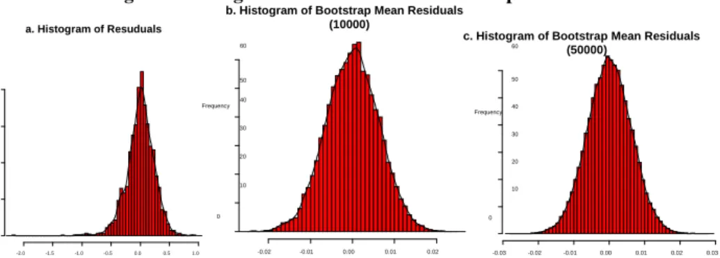
Finally we have utilized bootstrap sampling to get the confidence interval of each coefficient to ensure we have low bias in the estimates. We have modeled the Model 2 which is the classical Mincer earnings equation. Once we have fitted the regression model we got the residuals and the plot of residuals are given in figure 1 which gives a picture of bell-shaped frequency polygon. Now in bootstrap strategy we have taken samples of 10000, 20000, 30000, 40000, and 50000 to make sure we have a smoother bell-shaped curve of the residual plot (figure 1).
From the bootstrap sampling results we can perceive very low bias in the estimates with almost similar estimates of coefficients. The confidence intervals also satisfy the asymptotic convergence criteria.
Figure 1: Histograms of Residuals and Bootstrap Residuals
-2.0 -1.5 -1.0 -0.5 0.0 0.5 1.0 0.0 0.5 1.0 1.5 2.0 a. Histogram of Resuduals Residuals Frequency -0.02 -0.01 0.00 0.01 0.02 0 10 20 30 40 50 60
b. Histogram of Bootstrap Mean Residuals (10000)
Bootstrap Mean Residuals (b=10000) Frequency -0.03 -0.02 -0.01 0.00 0.01 0.02 0.03 0 10 20 30 40 50 60
Bootstrap Mean Residuals (b=50000) Frequency
c. Histogram of Bootstrap Mean Residuals (50000)
Table 4: Bootstrap Estimates with Confidence Interval and Bias Variable Bootstrap
coefficients
Standard error Confidence interval Bias (OLS-Bootstrap) YS 0.0467 0.0071 (0.0466, 0.0468) -1.569e-05 EXP 0.0269 0.0025 (0.0269, 0.0270) -4.500e-06 EXP2 -0.0003 0.0001 (-0.0003, -0.0003) 1.682e-07 ITQGV 0.0267 0.0046 (0.0267, 0.0268) 1.067e-05 TRAIN 0.1462 0.0146 (0.1459, 0.1463) -6.498e-05 GOVT -0.1063 0.0234 (-0.1066, -0.1060) -6.176e-05 CADET 0.1358 0.0316 (0.1354, 0.1362) 3.482e-05 PGA -0.4416 0.0211 (-0.4419, -0.4413) -5.352e-05 PNGA -0.3131 0.0342 (-0.3134, -0.3126) 7.872e-05 V. CONCLUSION
Our study found that the average return to education is around 18% for the secondary school teachers in Bangladesh which is not a surprise because the job the teachers are doing relates education and each extra year of education can bring them much higher position and as well higher salary. But when we introduced levels of education instead of years of schooling for capturing substantial non-linearity in rate of returns to education, it was found that returns increase with level of education. We found 9.49% returns to graduate educational level and 1.03% returns for postgraduate educational level. It also makes sense as most of the teachers in secondary level have graduate level degree. Among other factors, experience, teachers’ educational quality, training in job proved to have highly positive returns. Also, when schooling quality proxy was used, it was found that only Cadet Colleges have positive returns as compared to Govt, PGA and PNGA schools which indicates a comparatively low salary scale in Govt, PGA and PNGA schools. If we want teachers to have more returns from their job places we may want to re-arrange their salary scale throughout the country by comparing all kinds of institutions. The results presented in this paper may not necessarily reflect the true situation because of unavailability of lots of other factors responsible for the dynamic nature of the earnings-education mechanism.
ACKNOWLEDGMENT
The author gratefully acknowledges comments from Dr. Pk Md. Motiur Rahman and some other colleagues on an earlier draft of this paper.
REFERENCES
[1] Ahmed, M., Chakrabarty, S., Sengupta, S. and Rahman, P. M. (2004). “A Study of Secondary Education in Bangladesh and West Bengal”. Preliminary Draft, A Study Sponsored by the South Asian Network of Economic Research Institutes (SANEI).
[2] Asadullah, M. N. (2006). “Returns to Education in Bangladesh”. Education Economics, 14(4), 453-468.
[3] Cameron, A. C. and Trivedi, P. K. (2005) Microeconometrics: Methods and Applications, Cambridge University Press.
[4] Card, D. (2001). “Estimating the return to schooling: progress in some persistent econometric problems”. Econometrica, 69, no. 5.1127-1160.
[5] Hossain, M. (1990). Returns from education in rural Bangladesh, in: A. R. Khan and R. Sobhan (Eds) Trade, Planning and Rural Development: Essays in Honor of Nurul Islam (New York: St Martin’s Press).
[6] Hussain, Z. (2000). Bangladesh: education finance, in: Bangladesh Education Sector Review, vol.2 (Dhaka: University Press Limited).
[7] Mincer, J. (1974). Schooling, Experience, and Earnings, Columbia University Press: New York.
[8] Lemieux, T. (2006). The “Mincer Equation” Thirty Years After Schooling, Experience, and Earnings, in: Shoshana Grossbard (Ed) Jacob Mincer A Pioneer of Modern Labor Economics (Springer).