River discharge simulation using variable parameter McCarthy–Muskingum and wavelet-support vector machine methods

1

River Discharge Simulation Using Variable Parameter McCarthy–Muskingum and 1

Wavelet- Support Vector Machine Methods 2

Basant Yadav*1, Shashi Mathur2 3

1

Cranfield Water Science Institute, Cranfield University, 4

Cranfield MK43 0AL, UK 5

2

Department of Civil Engineering, Indian Institute of Technology Delhi, India 6

1*

Corresponding author email- [email protected] ; [email protected] 7

8

ABSTRACT 9

In this study an extended version of variable parameter McCarthy–Muskingum (VPMM) 10

method originally proposed by Perumal and Price (2013) was compared with the widely used 11

data based model namely support vector machine (SVM) and hybrid wavelet-support vector 12

machine (WA-SVM) to simulate the hourly discharge in Neckar River wherein significant 13

lateral flow contribution by intermediate catchment rainfall prevails during flood wave 14

movement. The discharge data from the year 1999 to 2002 has been used in this study. The 15

extended VPMM method has been used to simulate nine flood events of the year 2002 and 16

later the results were compared with SVM and WA-SVM models. The analysis of statistical 17

and graphical results suggest that the extended VPMM method was able to predict the flood 18

wave movement better than the SVM and WA-SVM models. A model complexity analysis 19

was also conducted which suggest that the two parameter based extended VPMM method has 20

less complexity than the three parameters based SVM and WA-SVM model. Further, the 21

model selection criteria also gives the highest values for VPMM in 7 out of 9 flood events. 22

The simulation of flood events suggested that both the approaches were able to capture the 23

underlying physics and reproduced the target value close to the observed hydrograph. 24

However, the VPMM models is slightly more efficient and accurate, than the SVM and WA-25

SVM model which are based only on the antecedent discharge data. The study captures the 26

Neural Computing and Applications, Available online 28 September 2018 DOI:10.1007/s00521-018-3745-1

Published by Springer. This is the Author Accepted Manuscript issued with: Creative Commons Attribution Non-Commercial License (CC:BY:NC 4.0). The final published version (version of record) is available online at DOI:10.1007/s00521-018-3745-1. Please refer to any applicable publisher terms of use.

2

current trend in the flood forecasting studies and showed the importance of both the 27

approaches (Physical and data based modeling). The analysis of the study suggested that 28

these approaches complements each other and can be used in accurate yet less computational 29

intensive flood forecasting. 30

31

Keywords- Flood forecasting, VPMM, SVM, Wavelet Transform 32

1. Introduction 33

Accurate forecasting of discharge is extremely important in flood management, reservoir 34

management and hydropower design. The accuracy in forecasting discharge depends on the 35

type of simulation model adopted and a review of literature shows that long term and short 36

term discharge forecasting models are being used extensively in various water management 37

problems such as flood control, drought management, water supply utilities operations, 38

irrigation supply management and sustainable development of water resources. In the last few 39

decades, researchers have proposed many models to improve the accuracy of discharge 40

forecasting. These models can be broadly classified as physically based, conceptual and data 41

driven models. A physically based model include as much of small-scale physics and natural 42

heterogeneity as is computationally possible by considering variables such as groundwater, 43

precipitation, evapotranspiration, initial soil moisture content and temperature (Loague and 44

Vander Kwaak, 2004). These can be further classified as hydraulic and hydrologic routing 45

methods. The hydrologic routing methods are widely used in the field practices since early 46

thirties and they have been developed essentially to overcome the tedious computations 47

involved in the hydraulic routing methods (Perumal et al., 2017). Among the many lumped 48

hydrological routing methods, the Muskingum method introduced by McCarthy (1938) is 49

well known in the literature (Chow et al., 1988). The Muskingum method was studied by 50

Ponce and Yevjevich (1978) resulting in the development of Variable Parameter Muskingum-51

3

Cunge (VPMC) method. However, the VPMC method was criticised for the mass 52

conservation problem (Perumal and Sahoo, 2008). To overcome this problem, Todini (2007) 53

revisited the original Muskingum-Cunge (MC) flood routing approach and suggested that the 54

error in mass conservation occurs due to the use of time variant parameters. Later, Price 55

(2009) proposed a nonlinear Muskingum method as an approximation of the one-dimensional 56

Saint-Venant equations and suggested a way out to include any uniformly distributed time-57

dependent lateral inflow along the river. Recently Perumal and Price (2013) proposed a fully 58

mass conservative approach to study the flood wave propagation in channels (without lateral 59

flow) named variable parameter Muskingum method based on the Saint-Venant equations. 60

Although, these methods successfully captured the flood wave movements and also tackled 61

the problem of mass conservation, the consideration of lateral flow along the river reach still 62

was the cause for erroneous river discharge prediction. A separate approach was suggested by 63

O’Donnell (1985) to include lateral flow in the Muskingum method assuming that the lateral 64

flow has the same form as the inflow hydrograph as pointed out by Perumal et al. (2001). 65

This concept was further studied by Karahan et al., (2014) using the approach of O’Donnell 66

(1985) to incorporate lateral flow and proposed a nonlinear Muskingum flood routing model. 67

This three parameter based semi-empirical Muskingum method has limitation about its 68

applicability to only those events which were similar to the observed past events. To 69

overcome this problem, Yadav et al., (2015) proposed an extended VPMM method 70

considering uniformly distributed lateral flow along the river reach. This study extended the 71

approach of Perumal and Price (2013) and successfully captured the significant amount of 72

lateral flow due to intervening catchment rainfall. Recently, Swain and Sahoo (2015) also 73

studied the fully mass conservative VPMM model and extended it to exclusively incorporate 74

the spatially and temporally distributed non-uniform lateral flow while routing the flood 75

events for compound river channel flows. 76

4

Although a physical method provide reasonable accuracy, their implementation and 77

calibration typically present various difficulties (Nayak et. al., 2007). Moreover, in situations 78

particularly in developing countries where the data about the processes to be modelled is 79

limited, physically based model cannot be built, or they are inadequate. A well-calibrated 80

conceptual model can also provide reasonable simulation accuracy, however, their uses are 81

limited, because entire physical process in the hydrologic cycle is mathematically formulated 82

in the conceptual models. Thus, they are composed of a large number of parameters making 83

the model very complicated and slow. This in turn leads to problems of over parameterization 84

(Beven, 2006) which may manifest itself in large prediction uncertainty (Uhlenbrook et al., 85

1999). In the last few decades, data driven techniques capable of handling large data sets 86

have been adopted while dealing with water resources problems. In forecasting of river 87

discharge, data-based hydrological methods are gaining popularity because they can be 88

developed very rapidly with requirement of minimal information (Yadav et al., 2016b). 89

Though they may lack the ability to provide a physical interpretation and insight into the 90

catchment processes, they are nevertheless able to forecast relatively accurate discharge 91

values (Adamowski and Sun, 2010). The lack of extensive data and cost of collection coupled 92

with inaccessibility of sites compels one to select models based on past recorded flow data 93

while simulating river flow variability (Kisi, 2008, Shiri and Kisi, 2010). Further, data-94

driven models that operate on an interrelationship between input-output data only without 95

capturing the complete dynamics of the system, may therefore be preferred in certain cases 96

(e.g., in contexts of limited data). 97

With the advent of computers and the availability of high computational facilities, 98

many researchers have employed data driven techniques while forecasting discharge (e.g., 99

Dawson and Wilby 1998; Sudheer et al. 2002; Shiri et al., 2012; Ghalkhani et al., 2013; 100

Badrzadeh et al., 2013; Rezaeianzadeh et al., 2014; Kasiviswanathan et al, 2016). Much 101

5

research has been carried out in the recent past on the use of artificial neural networks (ANN) 102

for discharge forecasting since it is reliable and promising and plethora of literature is 103

available with its applications. Study of hydrological processes using data based models 104

mainly depends on the time series of the considered process. The length of the time series is 105

also important as it captures the short term and long term trend of the process, which can also 106

help in accurate simulation and prediction of the future events. The neural network based 107

models were also used successfully for the trend analysis of time series (Maier and Dandy, 108

2000; Rafael et al., 2011; Lin et al., 2017). Similarly, Genetic programing (Koza, 1992) is 109

another data based approach which has been successfully applied to many studies in water 110

resources engineering problems. However, the most notable one was the support vector 111

machine (SVM), a kernel based technique based on the Vapnik–Chervonenkis (VC) theory 112

(Vapnik, 1995). The main advantage of this relatively new machine learning method is that it 113

not only possesses the strengths of ANN but is able to overcome the problems associated 114

with local minimum and network over fitting (ASCE Task Committee on Application of 115

Artificial Neural Networks in Hydrology, 2000). Further, despite the flexibility and 116

usefulness of data driven methods in modeling hydrological processes, they have some 117

drawbacks with highly non-stationary responses or seasonality (Cannas et al., 2006, Tiwari 118

and Chatterjee, 2010, Adamowski and Chan, 2011, Nourani et al., 2014). To handle such 119

problems a method called wavelet analysis (WA) has been used in various hydrological 120

studies. Sang (2013a) highlighted that the understanding of hydrologic series can be 121

improved from wavelet analysis. Recent application of wavelet analysis in hydrological 122

modeling (Kalteh, 2013, Suryanarayana et al., 2014, Agarwal et al., 2016, Yadav et al., 2017) 123

suggest that the WA approach provides a superior alternative to the data driven models and 124

can enhance the accuracy by developing the more detailed input–output combinations. In 125

light of the above facts, an attempt has been made herein to assess the abilities of the wavelet 126

6

based support vector machine to predict the discharge in a river reach where the lateral flow 127

is very significant. Further, we also intend to compare the two distinctively discharge 128

prediction approaches to suggest an accurate yet less complex discharge prediction method 129

for such a catchment conditions. The techniques were experimented on a 24.2 km stretch of 130

Neckar River between Rottweil and Oberndorf. 131

2. Methodology 132

2.1 Variable parameter McCarthy–Muskingum (VPMM) 133

The fully mass conservative VPMM was developed by Perumal and Price (2013). After a 134

decade of research, VPMM is capable to conserve volume absolutely and also follow the 135

heuristic assumption of the prism and wedge storage established by McCarthy (1938) in the 136

development of the classical Muskingum method. The method fundamentally makes use of a 137

parallel approach followed by Perumal (1994a, 1994b) in the development of the VPM 138

routing method. The VPMM method is developed from an approximation of the momentum 139

equation of the Saint-Venant equations. This approximation is applied directly to the one- 140

dimensional continuity equation of the Saint-Venant equations, leading to a fully 141

conservative routing method which has the same routing equation as the classical Muskingum 142

method proposed by McCarthy in (1938). The use of hydraulic principle in the development 143

of the VPMM method allow the characterization of the considered channel reach storage into 144

prism and wedge storage which complies with the heuristic assumption of McCarthy (1938) 145

who developed the Muskingum method. The equation derived in the VPMM method for the 146

travel time and weighting parameter is same as the classical Muskingum method and based 147

on the flow and channel characteristics. The equations governing the one-dimensional 148

unsteady flow in channels and rivers are given below (Perumal and Price (2013) as 149

7 0       t A x Q (1) 151 t y g x v g v x y S S_{f o}           1 (2) 152

The Eq. (1) and (2) represents the continuity and momentum equation, respectively. The 153

discharge at any section of the routing reach using the VPMM method can be obtained using 154

the equation as (Perumal and Price (2013) as 155 2 / 1 2 2 , 9 4 1 1 1                            M M o M o M dy dR B P F x y S Q Q (3) 156

where, tis the time; xis the distance along the channel; yis the flow depth; vis the average 157

cross-sectional velocity; Ais the cross-sectional area; Qrepresents the discharge; g is the 158

acceleration due to gravity; S_fis the frictional slope; Sois the bed slope;





longitudinal gradient of water profile;

 



 



wetted perimeter, top width and hydraulic radius corresponding to flow depth y_m. The 162

notation Q_Mis the average discharge at the mid-section of the reach at any time and Q_o,M is 163

the normal discharge at the midsection corresponding to flow depth ym andFMis the Froude 164

number. 165

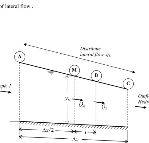
The developed VPMM method was further modified to account lateral flow in flood 166

routing study using the similar approach suggested by O’Donnell (1985). Though, the 167

fundamental principle remains same, lateral flow was incorporated in a distributed form 168

throughout the river stretch (Fig. 1). For the detailed explanation on the lateral flow 169

estimation approach readers can refer to Yadav et al., (2015). Accordingly, the lateral flow 170

8

hydrograph q_Lis assumed to have the similar shape as the inflow hydrograph and it is 171

supplied uniformly along the river stretch at each time interval. Hence, the original continuity 172

equation in the VPMM method is modified as 173 L q t A x Q       (4) 174

where, q_Lis the lateral flow per unit length of the channel. 175

The contribution of lateral flow in the river stretch is assumed to be perpendicular to the 176

channel reach, hence the channel flow receives no or very negligible momentum. 177

Accordingly, in the modified VPMM method the momentum equation (Eq. (2)) remains 178

unaltered. The modified continuity equation and the original momentum equation were 179

further solved to account the uniformly distributed lateral flow and the approach arrived at 180

following (Yadav et al., 2015) as 181 Lavg j i j i j i j i CQ CQ CQ Cq Q_₁1 ₁ 1 ₂  _{3 1} ₄ (5) 182

The coefficientsC₁,C₂,C3,C4 and qLavg are expressed as 183





















9

Considering the shape of lateral flow hydrograph as same as the inflow hydrograph, the 189

lateral flow rate q_L joining to the river stretch (discharge per unit length of the channel) is 190

obtained (Yadav et al., 2015) as 191 L V t I I q L N i L   



where, I is the inflow discharge at any time; L is the length of the river reach in meter; V_Lis 193

the volume of lateral flow . 194

195

196

Fig: 1. Concept diagram of VPMM method considering distributed lateral flow in river reach 197

(Yadav et al., 2015) 198

To calculate the discharge values at the downtream location, the VPMM method requires the 199

following data- Manning’s roughness value, Bed slope, River width (meter), Side slope and 200

Cross-sectional shape. The method also requires river dischrage data of the upstream gauging 201

station and rainfall data to calculate the lateral flow of the intervening catchment. As the 202 l Inflow Hydrograph, I Outflow Hydrograph, Q A C B M Distribute lateral flow, qL

10

VPMM method is a fully mass conservative, physically based method, it does not require any 203

calibration. The precipitation and discharge data of year 2002 was used in simulation of the 204

discharge at the downstream location. 205

206

2.2 Support vector machine 207

Vapnik et. al. (1995) proposed a kernel-based algorithm as support vector machine (SVM) 208

which has a function form like physical models, however, the level of complexity is to be 209

decided by the data used to train the model. The method was developed using the similar 210

principle like ANN, however by using a novel way to approximate various functions (i.e. 211

linear (LN), polynomial (PL), radial basis function (RBF), and sigmoid (SIG)) using the 212

method of structural risk minimization (opposite to the empirical risk minimization). A kernel 213

function is used to transform the data into higher dimensional feature space. The SRM 214

principle allows the method to have a good generalization ability for the unseen data. Let 215













n i R

x  represents 216

the input sample space andy_iRn for i1,...,l denotes respective target output, elements in 217

the training data set represented byl. Error tolerance level is fixed by a value of  (errors < 218

). The linear regression in SVM is estimated by solving the equation (7) as 219















wdenotes the normal vector, bis a bias, Crepresents a regularization constant,  is the error 222

tolerance level of the function, and the , are slack variables. 223

11

The support vector machine have variety of kernel function (mathematical function) 224

and its selection based on the problem at hand, which in turn has a direct impact on the 225

accuracy of the model (Yao et al., 2008). Various studies suggest that the RBF has higher 226

generalization ability and produce more accurate results than the other kernel types (Harpham 227

and Dawson, 2006; Yang et al., 2009; Tehrany et al., 2015, Yadav et al., 2017). A study by 228

Tehrany et al., (2014) suggested that RBF may produce less accurate results in case of longer 229

range extrapolation. However, RBF as a kernel function for SVM used by many researchers 230

in the past (Yu et al., 2004; Choy and Chan, 2003; Suryanarayana et al., 2014; Yadav et al., 231

2016a, Yadav et al., 2017, Yadav et al., 2018) and has been found to be suitable for 232

simulation and prediction studies. RBF is defined as 233









where X_i and X_j are vectors in the input space, such as the vectors of features computed 235

from training and testing.  is defined by, ₂

2 1



  for which  is the Gaussian noise level 236

of standard deviation. 237

The output of the SVM is critically dependent on the parameters such as regularization 238

constant

 

 

 

error procedure was used in the present study to optimize these parameters based on the 240

RMSE value. The trial continues by using different combinations of all three parameters till 241

the value of RMSE was minimized. Once the optimal parameters are obtained, the methods 242

requires time series of upstream and downstream gauging locations to simulate the discharge 243

values at the downstream location. The effect of lateral flow on the downstream discharge 244

values is automatically considered in the method as the lateral flow calculation is based on 245

the input and output discharge data. The time series data from the year 1999 to 2001 was used 246

for the training while the data from year 2002 was used for the testing. 247

12 248

2.3 Wavelet analysis 249

A wavelet analysis is based on Fourier analysis and was developed to analyze stationary and 250

non-stationary data. Wavelet decomposition is a technique used in case of non-periodic and 251

transient signals to extract the relevant time-frequency information by disintegrating the data 252

into low frequency and high frequency components. Wavelet decomposition breaks the signal 253

into low and high frequency components and utilizes the information hidden in the original 254

signal. The lower frequency components (approximation) are obtained using low pass filter 255

and captures the rapidly changing details of the signal. The higher frequency components 256

(details) are obtained using high pass filter to encompass the slowly changing features of the 257

signals. In this study, discrete wavelet transform (DWT) was used and the discharge time 258

series was decomposed into four resolution interval. Thus, some features of the subseries can 259

be seen more clearly than the original signal series. Though, DWT is able to decompose the 260

time series in many interval, it is important to note that higher number of resolution may also 261

slow down the computational speed. For each component a separate SVM model need to be 262

developed and the decomposed component may be given as the input for SVM. Later, the 263

output of the all the developed SVM (i.e. four in this case) will be summed to get the final 264

output in the form of recomposed time series. 265

There are two basic form of wavelet analysis, continuous wavelet transform (CWT) and 266

discrete wavelet transform (DWT). The continuous wavelet transform (CWT) of a signal x

 

is defined as follows (Kalteh, 2013): 268

 

 



13

where 

 

translation parameter. 271

The discrete wavelet transform (DWT) is defined as follows: 272

 

m and n is the resolution level and position which controls the scale and time; tis the time; 274

ais a specified fixed dilation step greater than 1; ₀is the location parameter that must be 275

greater than zero. The term am/2 in the above equation normalizes the functions. 276

The two form of wavelet has been used in many studies, however it was observed that 277

the CWT is computationally costly and requires large number of data. On the other hand the 278

development and application of DWT is much simpler and easy to use (Adamowski and 279

Chan, 2011; Kalteh, 2013). Therefore, DWT has been used in this study where a father 280

wavelet function used for the extraction of low frequency components while the high 281

frequency component is extracted by using a complementary of the father wavelet, a mother 282

wavelet function. The decomposition of the data series is represented by the approximation 283

series A_m and the detail seriesDm. Later, the both the approximation and detail series were 284

recomposed to get the final output of the model. 285

2.4. Evaluation criteria 286

The VPMM method was originally developed by Perumal and Price (2013) and further the 287

extended version considering the lateral flow was evaluated by Yadav et al., (2015). In the 288

flood forecasting study value of flood peak and its time of arrival is very important, hence in 289

this study three important evaluation criteria which is error in peak discharge (Qer), error in 290

time to peak (t_Qe) and error in volume (EVOL) are adopted. The criteria for error in volume 291

14

has different definition than the one proposed by Perumal and Price (2013) as in their method 292

the objective was to assess the error in mass conservation. However, in this study the lateral 293

inflow from the intervening catchment is very significant hence the mass reproduction at the 294

downstream location is bound to have higher value than the upstream location. Therefore, 295

this study evaluated the volume reproduction ability of the selected methods based on the 296

observed discharge at the downstream location. Further, the performance of VPMM, SVM 297

and WA-SVM was also evaluated using the statistical indicators like root mean square error 298

(RMSE), normalized mean square error (NMSE) and coefficient of determination (R2). The 299

aforementioned statistical indicator gives the interpretation about the overall reproduction 300

ability of the selected models, and may not provide the information that how the model 301

behaved throughout the flood event. Therefore, another evaluation criteria called absolute 302

average relative error (AARE) was adopted to assess the model performance at each 303

discharge ordinate. Furthermore, the performance of the selected methods was also evaluated 304

using graphical analysis where the closeness with which the proposed method reproduces the 305

benchmark solution, including the closeness of shape and size of the hydrograph, can be 306

measured using the Nash–Sutcliffe (NSE) efficiency criterion. The definition of RMSE, 307

NMSE, NSE and R2 can be found easily in the literature, however the definition for some of 308

the specific performance measures are given as follows: 309

Error in peak discharge (Qer) 310 100 1_        o s er Q Q Q (11) 311

Relative error in time to peak (t_Qe) 312 Qo Qs Qe t t t   (12) 313

15 Error in volume (EVOL)

314 100 1 1 1               





Absolute average relative error (AARE) 318 100 1 1   



where Qerrepresents the percentage error in simulated peak discharge; Qsis the simulated 320

peak discharge of the flood event at the downstream location (m3/s); Q_ois the observed peak 321

discharge of the flood event at the downstream location (m3/s); t_Qe is the relative error in 322

time to peak of the simulated flood event (hr); t_Qstime to peak of the simulated flood event 323

(hr); t_Qotime to peak of the observed flood event (hr); EVOLis the error in volume is 324

simulated flood event (%);Q_siis the ith ordinate of the simulated flood event (m3/s); Q_oiis the 325

ith ordinate of the observed flood event (m3/s) and Nis the total number of ordinates in the 326

flood event. 327

2.5 Evaluation of model complexity 328

The level of complexity of a specific model is tested using Akaike information criterion 329

(AIC) and model selection criteria (MSC). The most appropriate model based on the model 330

complexities is the one with the smallest values of the AIC and largest value of MSC. The 331

performance measures are also defined as; 332

16 p N i si oi Q N Q N AIC ln ( ) 2 1 2        _ 







where Q_srepresents the average simulated discharge and N_prepresents the number of model 335

parameters. 336

337

3. Study area and data 338

The research work as a part of this study was mainly performed on a part of the Neckar River 339

basin (Fig.2). This region is situated in the South- Western part of Germany in the state of 340

Baden Württemberg. The river in the catchment is unaffected by large hydropower 341

generation plants and other such water management structures or navigational reasons, which 342

are the most common reasons influencing the runoff characteristics of the catchment area. 343

The study area of this research is characterised by strong differences in altitude between the 344

foothills of the Black Forest in the west, the valley of the Neckar in the centre and once again 345

the steep ascent to the Schwäbische Alb in the east. The catchment consists of lots of narrow 346

valleys. There is a wide variety of vegetation in the study catchment. In the western part of 347

the catchment the soil is acidic and poor in minerals which supports only Spruce, fir and 348

beech trees. The same forest is also found in the sandy soil of Keuper. The pasture, meadows, 349

fruits, vines, ash tress, elm and lime trees are also found in the smaller pockets. The study 350

was conducted between the two initial observation stations Rottweil and Oberndorf on the 351

Neckar River. Distance between two stations is 24.2 km. The intermediate drainage area 352

between two stations is 235 km2 which is around 34 % of the total drainage area of Oberndorf 353

17

gauging station. The hourly amounts of precipitation used in the VPMM for the period from 354

1999 to 2002 are obtained from 3 precipitation stations which are distributed in and around 355

the catchment area. The data based modeling (SVM and WA-SVM) is based only on the 356

discharge time series from 1999 to 2002 (Fig. 3) which was provided by the University of 357

Stuttgart, Germany. The description of the study area is partly based on the description of 358

Das (2006) and CCHYDRO (1999).The discharge time series from 1999-2001 was used for 359

the training and, nine flood events from the year 2002 are selected for the comparative 360

analysis of the selected methods. The event selection was completely random but keeping in 361

mind that the peak discharge value should be high and lateral flow contribution must be more 362

than 10% in all events. The parameters for the application of extended VPMM were taken 363

from the study of Yadav et al., (2015). 364

365

Fig.2 Neckar catchment (IWS, Stuttgart) 366

18 367

Fig. 3 Time series at Rottweil (upstream) and Oberndorf (downstream) gauging stations 368

4. Results and discussions 369

4.1 Flood Routing Using VPMM, SVM and WA-SVM 370

The extended VPMM method and its parameters were obtained from the study conducted by 371

Yadav et al., (2015) for the same river stretch. The VPMM method under consideration has 372

only two parameters K and θ which depends on the cross sectional information and the flow 373

characteristics. The routing reach information such as bed slope and Manning’s roughness 374

value were obtained from the study reports of the Neckar river catchment, But the bed width 375

and side slope of the cross section (Table 1) of the channel reach is optimized by the ROPE 376

algorithm (Singh, 2008, Yadav et al., 2015). To avoid the influence of lateral inflow on the 377

parameter optimization process the flood event with a minimum lateral flow among the 9 378

events is considered for the analysis. The data based model namely SVM and WA-SVM were 379

developed using LIBSVM toolbox (Chang et al. 2011) to predict the discharge at the 380

downstream location. The Radial Basis Function was adopted as kernel function for SVM 381

and its parameters C and γ were obtained using a trial and error procedure where the trial 382

19

continues till the value of RMSE was minimized. Later, the SVM model was suitability 383

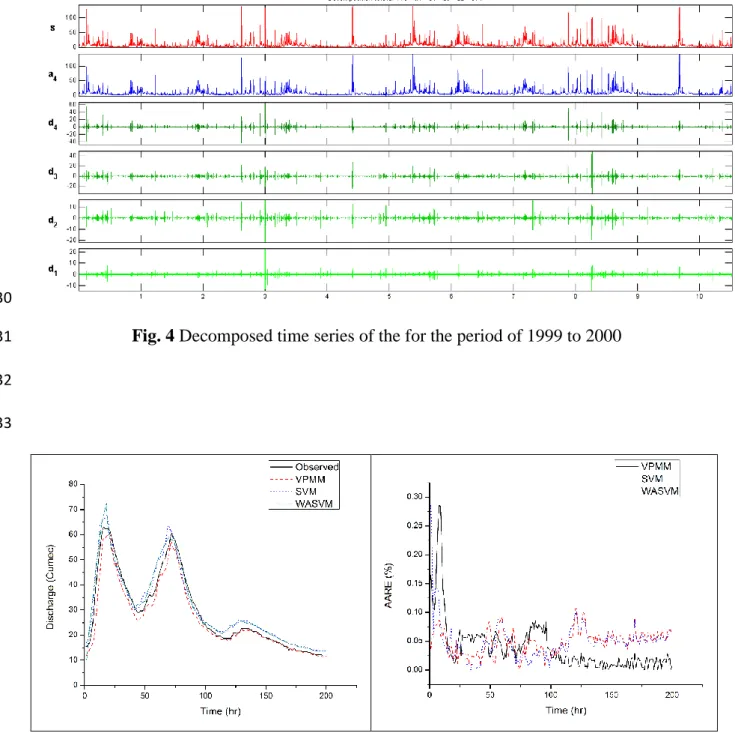
coupled with wavelet analysis (WA) which decomposes the input discharge time series using 384

DWT into approximation and detailed time series (Fig. 4). The parameters for SVM and WA-385

SVM has been presented in Table 2. After the model calibration (VPMM) or training (SVM, 386

WA-SVM) they were used to predict the discharge hydrograph of 9 flood events of the year 387

2002. 388

Table 1. Parameters for the development of VPMM method 389

Parameter Value

Manning’s roughness Bed slope

River width (meter) Side slope Cross-sectional shape 0.035 0.0034 8.417 1.035 Trapezoidal 390

Table 2. Optimal SVM and WA-SVM parameters for various decomposition series 391

Model Decomposed series best C best 

SVM 3.104 0.0412 WA-SVM Approximation series 42 0.0611 D1 series 3 0.0412 D2 series 3 0.0712 D3 series 7 0.0912 D4 series 9 0.0812 392

Table 3 presents the statistical analysis of the simulated hydrograph obtained by VPMM, 393

SVM and WA-SVM. The VPMM reproduced 7 out of 9 flood events with highest accuracy, 394

where the error measures like NMSE, RMSE values ranges between 0.018 to 0.083 and 1.471 395

20

(m3/s) to 4.301 (m3/s), respectively. Similarly the values for R2 and NSE ranges between 396

0.968 to 0.997 and 0.872 to 0.982, respectively. In case of SVM, the values obtained for 397

NMSE and RMSE were significantly high for most of the flood events and ranges between 398

0.046 to 0.176 and 2.932 (m3/s) to 5.918 (m3/s), respectively. The fitness criteria (R2 and 399

NSE) also follows the similar trend like error measures and ranges between 0.831 to 0.966 400

and 0.822 to 0.954, respectively. The inclusion of wavelet analysis has definitely improved 401

the accuracy of SVM and outperforms it in all flood events except 1, 3 and 9. Though, it is 402

evident from the statistical analysis that the VPMM method shows superiority over SVM and 403

WA-SVM, the reproduction of the downstream hydrographs for all the flood events by the 404

data based models are very close to the observed hydrographs. This argument is well 405

supported by the graphical representation of the observed and simulated hydrographs by 406

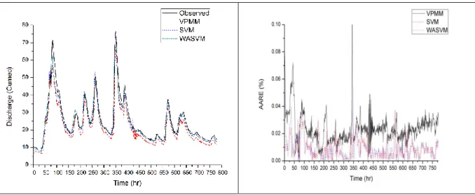
VPMM, SVM and WA-SVM (Fig. 5-13). It is also evident from these figures that the 407

absolute average relative error (AARE) of VPMM is very low. The AARE of SVM and WA-408

SVM is significantly higher than the VPMM, however WA-SVM shows relatively less error 409

than the SVM. These figures reveal that, under significant lateral flow conditions, the rising 410

limb, recession limb, and the peaks of the event-based flood hydrographs are all most well-411

reproduced by the VPMM, SVM and WA-SVM model. 412

Table. 3 Performance of VPMM, SVM and WA-SVM during the discharge prediction at the 413

Oberndorf gauging station 414

Flood event Method NMSE R2 RMSE (m3/s) NSE

1 VPMM _{0.028 0.984 3.421 0.948} SVM _{0.049 0.966 3.316 0.951} WASVM _{0.052 0.962 3.434 0.948} 2 VPMM _{0.083 0.980 4.197 0.916} SVM _{0.130 0.922 5.244 0.869} WASVM _{0.118 0.928 5.009 0.881} 3 VPMM 0.018 0.987 2.195 0.982 SVM _{0.129 0.948 5.918 0.870}

21 WASVM _{0.145 0.943 6.261 0.855} 4 VPMM _{0.020 0.981 1.471 0.979} SVM _{0.176 0.831 4.356 0.822} WASVM _{0.175 0.835 4.345 0.823} 5 VPMM _{0.071 0.968 4.301 0.928} SVM _{0.106 0.919 5.254 0.893} WASVM _{0.099 0.926 5.061 0.901} 6 VPMM _{0.030 0.987 2.415 0.970} SVM _{0.081 0.951 4.005 0.919} WASVM _{0.069 0.958 3.694 0.931} 7 VPMM _{0.035 0.970 3.579 0.965} SVM _{0.046 0.954 4.106 0.954} WASVM _{0.046 0.954 4.093 0.954} 8 VPMM _{0.128 0.976 4.545 0.872} SVM _{0.053 0.953 2.932 0.947} WASVM _{0.053 0.955 2.920 0.947} 9 VPMM _{0.015 0.997 1.469 0.985} SVM _{0.062 0.964 3.011 0.938} WASVM _{0.070 0.955 3.191 0.929} 415 416

Further analysis of the results indicates that the VPMM model works well in both the cases of 417

single or multi-peak peak flood events, however, data based models simulates the multi-peak 418

flood events (Events 1 and 8) better than VPMM. The reason for such outcome can be 419

attributed to the fact that the data based model performance primarily depends on the data 420

length. In case of flood event 8, the discharge time series length is around 800 hrs with 421

multiple peaks, which allowed the model to learn such occurrence properly. The study 422

suggest that, if the data based models are fed with sufficient length of discharge time series 423

data which encompass the variability in nature, they can simulate the discharge process with 424

reasonable accuracy. On the other hand, the reduction in accuracy of VPMM for these flood 425

events derives from the uncertainty in estimating the lateral flow which, mainly depends on 426

the initial soil moisture conditions. The spatial and temporal variability of soil moisture 427

22

content can have significant impact on the lateral flow estimation which in turn will reflect in 428

the simulation accuracy of the VPMM. 429

430

Fig. 4 Decomposed time series of the for the period of 1999 to 2000 431

432 433

Fig. 5 Routed hydrograph and AARE for flood event 1 using VPMM, SVM and WASVM. 434

23

Fig. 6 Routed hydrograph and AARE for flood event 2 using VPMM, SVM and WASVM. 435

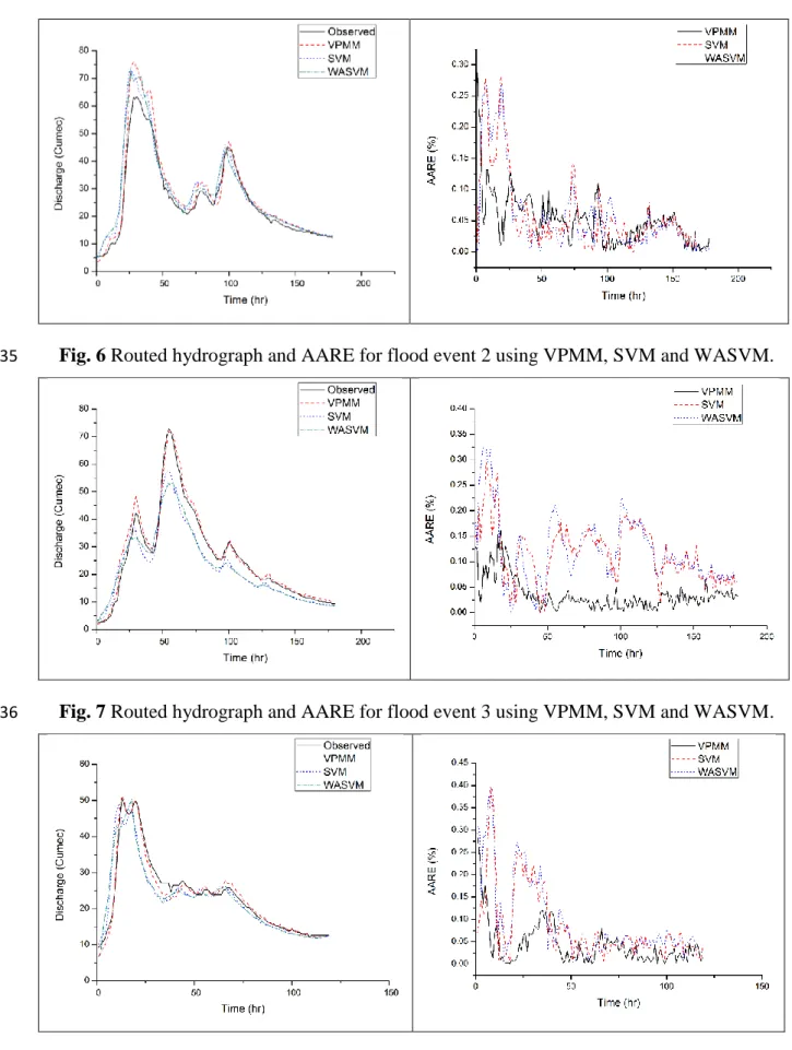
Fig. 7 Routed hydrograph and AARE for flood event 3 using VPMM, SVM and WASVM. 436

Fig. 8 Routed hydrograph and AARE for flood event 4 using VPMM, SVM and WASVM. 437

24

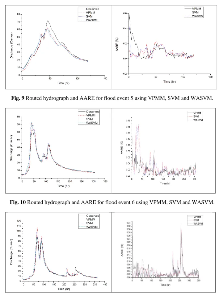
Fig. 9 Routed hydrograph and AARE for flood event 5 using VPMM, SVM and WASVM. 438

Fig. 10 Routed hydrograph and AARE for flood event 6 using VPMM, SVM and WASVM. 439

Fig. 11 Routed hydrograph and AARE for flood event 7 using VPMM, SVM and WASVM. 440

25

Fig. 12 Routed hydrograph and AARE for flood event 8 using VPMM, SVM and WASVM. 441

Fig. 13 Routed hydrograph and AARE for flood event 9 using VPMM, SVM and WASVM. 442

443

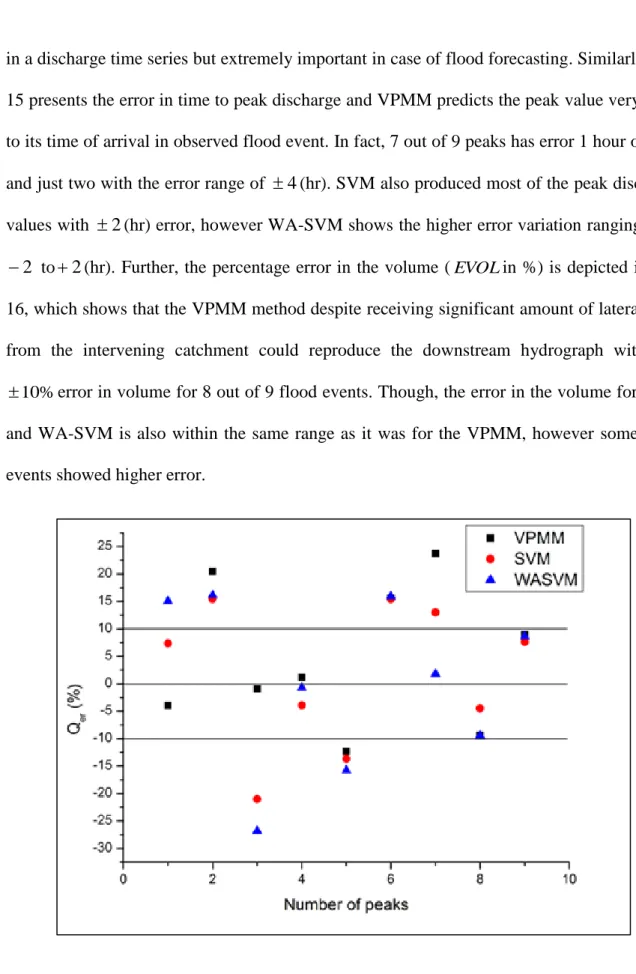
Further, considered methods in this study were also evaluated using the original criteria used 444

for the development of VPMM. The percentage error in the peak discharge (Qerin %), the 445

error in the time-to-peak discharge (t_Qein hr), and the percentage error in the volume (EVOL 446

in %) for all the 9 flood events has been depicted in Figs. 14, 15 and 16. It is evident from the 447

Fig. 14 that the VPMM method predicts most of the peak values (5 out of 9) within 10%

448

error and just 2 above the 20% error. However, in case of SVM and WA-SVM Qeris well 449

above the 10%range for most of the flood events. Which suggest that the data based 450

models may requires more training to predict such high discharge values which comes rarely 451

26

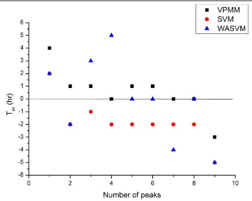
in a discharge time series but extremely important in case of flood forecasting. Similarly, Fig. 452

15 presents the error in time to peak discharge and VPMM predicts the peak value very close 453

to its time of arrival in observed flood event. In fact, 7 out of 9 peaks has error 1 hour or less, 454

and just two with the error range of 4(hr). SVM also produced most of the peak discharge 455

values with 2(hr) error, however WA-SVM shows the higher error variation ranging from 456

2

 to2(hr). Further, the percentage error in the volume (EVOLin %) is depicted in Fig. 457

16, which shows that the VPMM method despite receiving significant amount of lateral flow 458

from the intervening catchment could reproduce the downstream hydrograph with just 459

% 10

 error in volume for 8 out of 9 flood events. Though, the error in the volume for SVM 460

and WA-SVM is also within the same range as it was for the VPMM, however some flood 461

events showed higher error. 462

463 464

Fig. 14 Error in peak discharge prediction while using VPMM, SVM and WASVM 465

27 466

Fig. 15 Error in time to peak discharge prediction while using VPMM, SVM and WASVM 467

468

Fig. 16 variation of error in volume while using VPMM, SVM and WASVM 469

470

4.2 Level of Complexity in VPMM, SVM amd WA-SVM 471

28

The method under consideration were also evaluated to assess the level of complexity while 472

desgining the model for discharge prediction. Table 4 presents the model complexity analysis 473

of VPMM, SVM and WA-SVM based on the number of parameter each model requires to be 474

tuned while designing the model for a specific application. The VPMM method has only two 475

parameters that is K and θ while the SVM has three parameters namely regularization 476

constant (C), insensitive loss function (ε), and parameter of radial basis function (γ). It is 477

evident from the table that the Akaike information criterion (AIC) is lowest while using 478

VPMM, in comparison to SVM and WASVM for most of the flood events. Similarly the 479

model selection criteria (MSC) value is highest for 8 out of 9 flood events when VPMM is 480

used, however it decreased significantly for SVM and WA-SVM. 481

482

Table 4. Akaike information criterion (AIC) and model selection criteria (MSC) for VPMM, 483 SVM and WA-SVM 484 Flood Event AIC MSC VPMM SVM WA-SVM VPMM SVM WA-SVM 1 1555.64 1545.19 1559.21 -0.02 -0.030 -0.030 2 1437.02 1518.28 1501.94 -0.022 -3.203 -5.220 3 1221.69 1580.78 1601.07 -0.022 0.233 -4.822 4 664.62 924.92 924.34 -0.033 -0.391 -2.030 5 919.94 969.57 960.66 -0.033 -0.805 -4.307 6 2303.60 2616.07 2566.52 -0.013 -0.610 -3.529 7 3088.30 3190.54 3188.27 -0.011 -0.040 -2.250 8 7560.23 6878.02 6871.93 -0.005 1.348 -2.286 9 1789.87 2192.25 2224.57 -0.014 -0.889 -3.288 485 486 5. Conclusion 487

29

In this study two approaches were used to predict the downstream discharge of Neckar River 488

in which VPMM is a physically based method and the SVM is data based method. Further, 489

wavelet analysis was also used to develop a hybrid WA-SVM model. The study was 490

conducted using 9 flood events from the year 2002 which is characterised of having 491

significant lateral flow joining from the intervening catchment, which in general is difficult to 492

model due to its spatial and temporal variability. Based on the analysis of statistical and 493

graphical results, it is inferred that the extended physically based variable parameter 494

Muskingum routing method (VPMM) is more robust and reliable than the data based models 495

like SVM and WA-SVM, when used to predict the discharge in a river reach with significant 496

lateral flow joining between the upstream and downstream gauging stations. However, it is 497

also evident from the analysis that the data based models successfully captured the flood 498

wave moment phenomenon and were able to map the process even with lateral flow, hence 499

reproduced the discharge hydrograph close to the observed hydrograph at the downstream 500

location. Further, based on the Akaike information criterion (AIC) and model selection 501

criteria (MSC), it can be concluded that the VPMM model is relatively less complex than the 502

SVM and WA-SVM. Lastly, it can be summarised that the physically based extended VPMM 503

method can predict the discharge hydrograph better than the data based mode, however, in 504

case of multi-peak flood events with sufficient discharge data, the later performed better than 505 VPMM method. 506 507 Acknowledgement 508

The author thankfully acknowledge the support and motivation provided by Prof. M. 509

Perumal. The necessary data to conduct this study was provided by TU Stuttgart, Germany. 510

The financial support to conduct this study was provided by IIT Delhi, India. 511

512

Conflict of Interest Statement 513

30

We confirm that this manuscript has not been published elsewhere and is not under 514

consideration by another journal. All the authors have approved the manuscript and agree 515

with the submission to Neural Computing and Applications Journal. The financial support 516

was provided by IIT Delhi. The authors have no conflict of interest to declare. 517

References 518

Adamowski, J., & Sun, K., 2010. Development of a coupled wavelet transform and neural 519

network method for flow forecasting of non-perennial rivers in semi-arid watersheds. Journal 520

of Hydrology, 390(1), 85-91. 521

522

Adamowski, J., & Chan, H. F., 2011. A wavelet neural network conjunction model for 523

groundwater level forecasting. Journal of Hydrology, 407(1), 28-40. 524

525

ASCE Task Committee on Application of Artificial Neural Networks in Hydrology, 2000. 526

527

Agarwal, A., Maheswaran, R., Kurths, J., & Khosa, R. 2016. Wavelet Spectrum and self-528

organizing maps-based approach for hydrologic regionalization-a case study in the western 529

United States. Water Resources Management, 30(12), 4399-4413. 530

531

Badrzadeh, H., Sarukkalige, R., & Jayawardena, A. W., 2013. Impact of multi-resolution 532

analysis of artificial intelligence models inputs on multi-step ahead river flow forecasting. 533

Journal of Hydrology, 507, 75-85. 534

535

Beven, K., 2006. A manifesto for the equifinality thesis. Journal of hydrology, 320(1), 18-36. 536

CC-HYDRO, 1999. Impact of Climate Change on River Basin Hydrology under Different 537

Climatic Conditions, March 1999. Universität Stuttgart, Germany. 538

539

Borges, R. V., Garcez, A. D. A., & Lamb, L. C., 2011. Learning and representing temporal 540

knowledge in recurrent networks. IEEE Transactions on Neural Networks, 22(12), 2409-541

2421. 542

31

Cannas, B., Fanni, A., See, L., & Sias, G., 2006. Data preprocessing for river flow forecasting 544

using neural networks: wavelet transforms and data partitioning. Physis and Chemistry of the 545

Earth 31 (18), 1164–1171. 546

547

Chang C. C., & Lin C. J., 2011. LIBSVM: a library for support vector machines. ACM Trans. 548

Intell. Syst. Technol. 2 (3) 27. 549

550

Chow, V.T., Maidment, D.R., & Mays, L.W., 1988. Applied Hydrology. McGraw-Hill, New 551

York. 552

553

Choy K., & Chan C., 2003. Modelling of river discharges and rainfall using radial basis 554

function networks based on support vector regression, Int. Journal of System Science, 34 (1) 555

763–773 556

557

Das, T., 2006. The Impact of Spatial Variability of Precipitation on the Predictive 558

Uncertainty of Hydrological Models, Ph.D. Dissertation No. 154, University of Stuttgart. 559

560

Dawson C.W., & Wilby R., 1998. An artificial neural network approach to rainfall–runoff 561

modeling. Hydrological Sciences Journal, 43 (1), pp. 47–66. 562

563

Ghalkhani, H., Golian, S., Saghafian, B., Farokhnia, A., & Shamseldin, A., 2013. Application 564

of surrogate artificial intelligent models for real‐time flood routing. Water and Environment 565

Journal, 27(4), 535-548. 566

567

Harpham, C., & Dawson, C. W., 2006. The effect of different basis functions on a radial basis 568

function network for time series prediction: a comparative study. Neurocomputing, 69(16), 569

2161-2170. 570

571

Kalteh, A. M., 2013. Monthly River flow forecasting using artificial neural network and 572

support vector regression models coupled with wavelet transform. Computers & 573

Geosciences, 54, 1-8. 574

575

Karahan, H., Gurarslan, G., & Geem, Z. W., 2015. A new nonlinear Muskingum flood 576

routing model incorporating lateral flow. Engineering Optimization, 47(6), 737-749. 577

32 578

Kasiviswanathan, K. S., He, J., Sudheer, K. P., & Tay, J. H., 2016. Potential application of 579

wavelet neural network ensemble to forecast streamflow for flood management. Journal of 580

Hydrology, 536, 161-173 581

582

Kisi, O., 2008. River flow forecasting and estimation using different artificial neural network 583

techniques. Hydrological Research, 39 (1), 27–40. 584

585

Koza, J. R., 1992. Genetic programming: on the programming of computers by means of 586

natural selection (Vol. 1). MIT press. 587

588

Lin, T., Guo, T., & Aberer, K., 2017. Hybrid neural networks for learning the trend in time 589

series. In Proceedings of the Twenty-Sixth International Joint Conference on Artificial 590

Intelligence, IJCAI-17 (pp. 2273-2279). 591

592

Loague, K., & VanderKwaak, J. E., 2004. Physics‐based hydrologic response simulation: 593

Platinum bridge, 1958 Edsel, or useful tool. Hydrological Processes, 18(15), 2949-2956. 594

Maier, H. R., & Dandy, G. C., 2000. Neural networks for the prediction and forecasting of 595

water resources variables: a review of modelling issues and applications. Environmental 596

modelling & software, 15(1), 101-124. 597

598

McCarthy, G.T., 1938. The unit hydrograph and flood routing. In: Conference of North 599

Atlantic Div., U.S. Army Corps of Engineers. 600

601

Nourani, V., Baghanam, A. H., Adamowski, J., & Kisi, O., 2014. Applications of hybrid 602

wavelet–Artificial Intelligence models in hydrology: A review. Journal of Hydrology, 514, 603

358-377. 604

605

O’Donnell, T., 1985. A direct three-parameter Muskingum procedure incorporating lateral 606

inflow. Hydrological Science Journal. 30 (4), 479–496. 607

608

Nayak, P. C., Sudheer, K. P., & Jain, S. K., 2007. Rainfall‐runoff modeling through hybrid 609

intelligent system. Water Resources Research, 43(7). 610

33

Perumal, M., 1994a. Hydrodynamic derivation of a variable parameter Muskingum method: 612

1. Theory and solution procedure. Hydrological sciences journal, 39(5), 431-442. 613

614

Perumal, M., 1994b. Hydrodynamic derivation of a variable parameter Muskingum method: 615

2. Verification. Hydrological sciences journal, 39(5), 443-458. 616

617

Perumal, M., O’Connell, P.E., & Ranga Raju, K.G., 2001. Field applications of a variable 618

parameter Muskingum method. Journal of Hydraulic Engineering. 6 (3), 1084-0699/01/0003-619

0196-0207. 620

621

Perumal, M., & Sahoo, B., 2008. Volume conservation controversy of the variable parameter 622

Muskingum–Cunge method. Journal of Hydraulic Engineering, 134(4), 475-485. 623

624

Perumal, M., & Price, R.K., 2013. A fully volume conservative variable parameter 625

McCarthy-Muskingum method: theory and Verification. Journal of Hydrology. 502, 89–102. 626

627

Perumal, M., Tayfur, G., Rao, C. M., & Gurarslan, G., 2017. Evaluation of a physically based 628

quasi-linear and a conceptually based nonlinear Muskingum methods. Journal of 629

Hydrology, 546, 437-449. 630

631

Ponce, V. M., & Yevjevich, V., 1978. Muskingum-Cunge method with variable parameters. 632

Journal of the Hydraulics Division, 104(12), 1663-1667. 633

634

Price, R. K., 2009. Volume-conservative nonlinear flood routing. Journal of Hydraulic 635

Engineering, 135(10), 838-845. 636

637

Rezaeianzadeh, M., Tabari, H., Yazdi, A. A., Isik, S., & Kalin, L., 2014. Flood flow 638

forecasting using ANN, ANFIS and regression models. Neural Computing and Applications, 639

25(1), 25-37. 640

641

Sang, Y. F., 2013. A review on the applications of wavelet transform in hydrology time series 642

analysis. Atmospheric research, 122, 8-15. 643

34

Shiri, J., & Kisi, O., 2010. Short-term and long-term streamflow forecasting using a wavelet 645

and neuro-fuzzy conjunction model. Journal of hydrology, 394(3), 486-493. 646

647

Shiri, J., Kişi, Ö., Makarynskyy, O., Shiri, A. A., & Nikoofar, B., 2012. Forecasting daily 648

stream flows using artificial intelligence approaches. ISH Journal of Hydraulic Engineering, 649

18(3), 204-214. 650

651

Singh, S.K., 2008. Robust Parameter Estimation in Gauged and Ungauged Basins, Ph.D. 652

dissertation No. 198, University of Stuttgart. 653

654

Sudheer, K. P., Gosain, A. K., & Ramasastri, K. S., 2002. A data-driven algorithm for 655

constructing artificial neural network rainfall–runoff models. Hydrological Processes, 16, 656

1325–1330. 657

658

Suryanarayana, C., Sudheer, C., Mahammood, V., & Panigrahi, B. K., 2014. An integrated 659

wavelet-support vector machine for groundwater level prediction in Visakhapatnam, India. 660

Neurocomputing, 145, 324-335. 661

662

Swain, R., & Sahoo, B., 2015. Variable parameter McCarthy–Muskingum flow transport 663

model for compound channels accounting for distributed non-uniform lateral flow. Journal of 664

Hydrology, 530, 698-715. 665

666

Tehrany, M. S., Pradhan, B., & Jebur, M. N., 2014. Flood susceptibility mapping using a 667

novel ensemble weights-of-evidence and support vector machine models in GIS. Journal of 668

Hydrology, 512, 332-343. 669

670

Tehrany, M. S., Pradhan, B., Mansor, S., & Ahmad, N., 2015. Flood susceptibility 671

assessment using GIS-based support vector machine model with different kernel 672

types. Catena, 125, 91-101. 673

674

Tiwari, M.K., & Chatterjee, C., 2010. Development of an accurate and reliable hourly flood 675

forecasting model using wavelet–bootstrap–ANN (WBANN) hybrid approach. Journal of 676

Hydrology 1 (394), 458–470. 677

35 678

Todini, E., 2007. A mass conservative and water storage consistent variable parameter 679

Muskingum-Cunge approach. Hydrology and Earth System Sciences Discussions, 4(3), 1549-680

1592. 681

682

Uhlenbrook, S., Seibert, J., Leibundgut, C., & Rodhe, A., 1999. Prediction uncertainty of 683

conceptual rainfall–runoff models caused by problems to identify model parameters and 684

structure. Hydrological Sciences Journal 44, 779–798. 685

686

Vapnik, V. N., 1995. The Nature of Statistical Learning Theory. Springer-Verlag, New York, 687

USA. 314 p. 688

689

Yadav, B., Mathur, S., & Yadav, B. K. 2018. Data-based modelling approach for variable 690

density flow and solute transport simulation in a coastal aquifer. Hydrological Sciences 691

Journal, 1-17. 692

693

Yadav, B., & Eliza, K., 2017. A hybrid wavelet-support vector machine model for prediction 694

of Lake water level fluctuations using hydro-meteorological data. Measurement, 103, 294-695

301. 696

697

Yadav, B., Ch, S., Mathur, S., & Adamowski, J., 2016a. Estimation of in-situ bioremediation 698

system cost using a hybrid Extreme Learning Machine (ELM)-particle swarm optimization 699

approach. Journal of Hydrology, 543, 373-385. 700

701

Yadav, B., Ch, S., Mathur, S., & Adamowski, J. 2016b. Discharge forecasting using an online 702

sequential extreme learning machine (OS-ELM) model: a case study in Neckar River, 703

Germany. Measurement, 92, 433-445. 704

705

Yadav, B., Perumal, M., & Bardossy, A., 2015. Variable parameter McCarthy–Muskingum 706

routing method considering lateral flow. Journal of Hydrology, 523, 489-499. 707

708

Yao, X., Tham, L., & Dai, F., 2008. Landslide susceptibility mapping based on support 709

vector machine: a case study on natural slopes of Hong Kong, China. Geomorphology 101, 710

572–582. 711

36 712

Yang, J., L., Y., Tian, Y., Duan, L., & Gao, W. Group-sensitive multiple kernel learning for 713

object categorization. In ICCV, 2009. 714

715

Yu X., Liong S., & Babovic V., 2004. EC-SVM approach for real-time hydrologic 716

forecasting. Journal of Hydroinformatics, 6 (3) 209–223. 717