NBER WORKING PAPER SERIES
THE WEALTH-CONSUMPTION RATIO Hanno Lustig
Stijn Van Nieuwerburgh Adrien Verdelhan Working Paper 13896
http://www.nber.org/papers/w13896
NATIONAL BUREAU OF ECONOMIC RESEARCH 1050 Massachusetts Avenue
Cambridge, MA 02138 March 2008
This paper circulated before as The Wealth-Consumption Ratio: A Litmus Test for Consumption-Based Asset Pricing Models. The authors would like to thank Dave Backus, Geert Bekaert, John Campbell, John Cochrane, Ricardo Colacito, Pierre Collin-Dufresne, Bob Dittmar, Greg Duffee, Darrell Duffie, Robert Goldstein, Lars Peter Hansen, John Heaton, Dana Kiku, Ralph Koijen, Martin Lettau, Francis Longstaff, Sydney Ludvigson, Thomas Sargent, Kenneth Singleton, Stanley Zin, and participants of the NYU macro lunch, seminars at Stanford GSB, NYU finance, BU, the University of Tokyo, LSE, the Bank of England, FGV, MIT Sloan, Purdue, LBS, Baruch, Kellogg, Chicago GSB, and conference participants at the SED in Prague, the CEPR meeting in Gerzensee, the EFA meeting in Ljubljana, the AFA and AEA meetings in New Orleans, the NBER Asset Pricing meeting in Cambridge, and the NYU Five Star Conference for comments. This work is supported by the National Science Foundation under Grant No 0550910. The views expressed herein are those of the author(s) and do not necessarily reflect the views of the National Bureau of Economic Research.
NBER working papers are circulated for discussion and comment purposes. They have not been peer-reviewed or been subject to the review by the NBER Board of Directors that accompanies official NBER publications.
© 2008 by Hanno Lustig, Stijn Van Nieuwerburgh, and Adrien Verdelhan. All rights reserved. Short sections of text, not to exceed two paragraphs, may be quoted without explicit permission provided that full credit, including © notice, is given to the source.
The Wealth-Consumption Ratio
Hanno Lustig, Stijn Van Nieuwerburgh, and Adrien Verdelhan NBER Working Paper No. 13896
March 2008, Revised January 2010
JEL No. E21,G10,G12
ABSTRACT
We set up an exponentially affine stochastic discount factor model for bond yields and stock returns in order to estimate the prices of aggregate risk. We use the estimated risk prices to compute the no-arbitrage price of a claim to aggregate consumption. The price-dividend ratio of this claim is the wealth-consumption ratio. Our estimates indicate that total wealth is much safer than stock market wealth. The consumption risk premium is only 2.2 percent, substantially below the equity risk premium of 6.9 percent. As a result, the average US household has more wealth than one might think; most of it is human wealth. A large fraction of the variation in total wealth can be traced back to changes in long-term real interest rates. Contrary to conventional wisdom, we find that events in bond markets, not stock markets, matter most for understanding fluctuations in total wealth.
Hanno Lustig
UCLA Anderson School of Management 110 Westwood Plaza, Suite C413
Los Angeles, CA 90095-1481 and NBER
[email protected] Stijn Van Nieuwerburgh Stern School of Business New York University 44 W 4th Street, Suite 9-120 New York, NY 10012 and NBER
Adrien Verdelhan
MIT Sloan School of Management Department of Finance
50 Memorial Drive, E52-436 Cambridge, MA 02142 and NBER
Stock returns have played a central role in the development of modern asset pricing theory. Yet, stock market wealth is only 2 percent of total household wealth according to our estimates. Real estate, non-corporate businesses, other financial assets, durable consumption goods, and especially human wealth constitute the bulk of total household wealth. The conventional view in asset pricing is that stock market returns are a good proxy for the returns on that remaining 98 percent of the total wealth portfolio (Stambaugh 1982). Much of the empirical work in asset pricing uses the return on the stock market as a stand-in for the total wealth return. Ever since the seminal work of Mehra and Prescott (1985), much of the theoretical work in the equity premium literature models equity as a claim to aggregate consumption. Our results challenge this conventional approach. To understand variation in total wealth, we should look at bond markets, not stock markets.
We measure total wealth and its price-dividend ratio, the wealth-consumption ratio, by comput-ing the no-arbitrage price of a claim to the aggregate consumption stream. Our measurement does not rely on specifying the preferences of agents, only on the dynamics of aggregate consumption growth. To value this claim, we estimate from stock returns and bond yields the prices of aggregate risk that US households face. We assume that the aggregate consumption growth innovations that are not spanned by traded assets, are not priced.
US households have more wealth than one might think. Our estimates imply that the represen-tative agent had $3 million of total wealth in 2006. The dynamics of the wealth-consumption ratio are largely driven by the dynamics of real bond yields. As a result, we find that between 1979 and 1981 when real interest rates rose, $533,000 of per capita wealth (in 2006 dollars) was destroyed. Afterwards, as real yields fell, real per capita wealth increased without interruption from $790,000 in 1981 to $3 million in 2006. The timing of the 1979-81 wealth destruction did not coincide with the stock market crash of 1973-74. Likewise, total wealth was hardly affected by the spectacular decline in the stock market that started in 2000.
We estimate a low consumption risk premium and a high wealth-consumption ratio. The average household’s wealth portfolio behaves more like a long-maturity real bond than like equity, for three reasons. First, the total wealth portfolio earns a low risk premium of around 2.2 percent per year, compared to a much higher equity risk premium of 6.9 percent. As a result, the wealth-consumption ratio is much higher, 87 on average, than the price-dividend ratio on equity, 27 on average. Second, the wealth-consumption ratio is less volatile than the price-dividend ratio: its standard deviation is 17 percent versus 27 percent. The return on total wealth has a volatility that is 9.8 percent per year, compared to 16.7 percent for equity returns. Third, the lower variability in the wealth-consumption ratio indicates less variation in expected future total wealth returns. Hence, there is less predictability in total wealth returns than in equity returns. Moreover, most of the variation in future expected total wealth returns is variation in future expected risk-free rates, and not variation in future expected excess returns.
What explains these results is that the consumption risk premium, defined as the risk premium on a claim to stochastically growing aggregate consumption, ends up looking quite similar to the risk premium on a claim to deterministically growing aggregate consumption. The latter claim is a perpetuity with deterministically growing real cash-flows. Its risk premium is the bond risk premium. The risk premia on the risky consumption claim and the real perpetuity are exactly identical if neither innovations to current nor to future consumption growth are priced. These two conditions are approximately satisfied in the data: the consumption cash flow risk accounts for only 15 percent of the consumption risk premium while the bond risk premium accounts for the remaining 85 percent. The resulting spread in risk premia between the two claims is only 0.33 percent per year. These findings are not a foregone conclusion. To allow for priced innovations to future consumption growth, the state vector includes variables that have been shown to predict consumption growth such as the short-term interest rate and the slope of the yield curve. To allow for priced innovations to current consumption growth, we make sure our model prices the returns on a factor mimicking portfolio for consumption growth. Next, we check whether the pricing of consumption innovations that are not spanned by innovations to bond yields or stock returns can overturn our results. Finally, because our results are not driven by the lower volatility of consumption growth, differences between the total wealth portfolio and equity cannot be eliminated by modeling equity as a leveraged claim to aggregate consumption.
Our estimates imply that the real perpetuity with deterministic consumption growth trades at a 37 percent premium to the risky consumption claim. Alvarez and Jermann (2004) show that this premium measures the marginal cost of consumption fluctuations in a large class of representative agent asset pricing models. The representative household would be willing to give up 37 percent of the last unit of annual consumption in exchange for a marginal reduction in aggregate consumption growth risk. This number, which is estimated without taking a stance on preferences, is useful in evaluating the plausibility of structural asset pricing models. After all, it reflects the representative agent’s attitudes towards consumption risk which are at the heart of these models. More generally, because the primitives in the leading representative agent asset pricing models are the preferences and the dynamics of aggregate consumption growth, the moments of returns on the consumption claim should be the most informative for testing these models. In contrast, the dividend growth dynamics of stocks can be altered without affecting equilibrium allocations or prices of any traded assets other than stocks; modeling them entails more degrees of freedom.1 Hence, the fact that several competing models with different primitives match the same moments of equity returns should not come as a surprise. Our approach is to study the primitive asset pricing moments of these models and to compare them to the same moments we measure in the data.2
1Although many model equity as a levered up claim to aggregate consumption, following Abel (1999), they fail
to impose restrictions on the long-run behavior of dividends relative to consumption.
The conventional view in modern asset pricing is that equity inherits its risk-return properties from the total wealth portfolio. In this view, equity is risky simply because the total wealth portfolio is. From this perspective, the theoretical challenge is to explain why the price of aggregate consumption growth risk is high and volatile. The first model we study, the external habit model (EH) of Campbell and Cochrane (1999), provides a preference-based answer to this challenge.3 In this model, the consumption and equity claim are similar and the price-dividend ratio on equity and the wealth-consumption ratio are almost identical, even though consumption and dividend growth are not highly correlated.4 A version of the EH model that is calibrated to match the equity premium, produces a consumption risk premium of 10.7 percent per annum, while the average wealth-consumption ratio is only 12, 7.25 times smaller than our estimate. Moreover, the wealth-consumption ratio implied by the EH model is almost twice as volatile as the one we have estimated in the data. All of this variation reflects variation in risk premia and not risk-free rates, again inconsistent with our findings. As a result, the EH model dramatically overstates the representative agent’s aversion to aggregate consumption fluctuations: the implied marginal cost of consumption risk is 20 times too high.
Our no-arbitrage model prices bonds and stocks rather well, but the estimates lead us to conclude that the total wealth portfolio is more like a portfolio of bonds than stocks. The correlation between realized total wealth returns and stock returns is only 0.12, while the correlation with realized 5-year government bond returns is 0.50. These estimates support the view that equity simply is quite different from the the total wealth portfolio. From our perspective, the new challenge to theorists is to explain why equity is so different from the consumption claim, yet still perceived to be so risky.
The second model we study provides one possible answer to this new challenge. The long-run risk model (LRR) of Bansal and Yaron (2004) makes the dividend claim (equity) much more exposed to shocks to the persistent component of aggregate consumption growth than the con-sumption claim.5 As a result, the LRR model generates a much higher and less volatile wealth-consumption ratio than the price-dividend ratio on equity. The average wealth-wealth-consumption ratio
to highlight the key role of the wealth-consumption ratio.
3Early contributions in the habit literature include Abel (1990), Constantinides (1990), Ferson and Constantinides
(1991), Abel (1999). See Menzly, Santos, and Veronesi (2004) and Wachter (2006) for more recent contributions. Verdelhan (2008) explores the international finance implications and Chen, Collin-Dufresne, and Goldstein (2008) the implications for credit spreads. Chen and Ludvigson (2007) estimate the habit process for a class of EH models.
4See graph on page 220 in Campbell and Cochrane (1999).
5Parker and Julliard (2005) and Malloy, Moskowitz, and Vissing-Jorgensen (2009) measure long-run risk based
on leads and long-run impulse responses of consumption growth. Bansal, Kiku, and Yaron (2007) estimate the long-run risk model. Piazzesi and Schneider (2006) study its implications for the yield curve, Bansal, Dittmar, and Lundblad (2005) study the implications for the cross-section of equity portfolios, Benzoni, Collin-Dufresne, and Goldstein (2008) for options, and Colacito and Croce (2005) and Bansal and Shaliastovich (2007) for international finance. Chen, Favilukis, and Ludvigson (2008) estimate a model with recursive preferences, while Bansal, Gallant, and Tauchen (2007) estimate both long-run risk and external habit models, and Yu (2007) compares correlations between consumption growth and stock returns across the two models.
in the benchmark LRR model is 87, the same value we estimate in the data, which shows that our numbers are consistent with a standard equilibrium asset pricing model. Most of the variation in the wealth-consumption ratio comes from variability in interest rates, again consistent with the data. However, the LRR mechanism implies more predictability in aggregate consumption growth than is observed in the data.6
We turn now to the link to the previous literature. The properties of the average household’s total portfolio are crucial for the evaluation of dynamic asset pricing theories. Roll (1977) stresses that the total wealth return is the right pricing factor in the Capital Asset Pricing Model. Similarly, Campbell (1993) shows that current and future total wealth returns substitute for consumption growth as pricing factors in the Intertemporal CAPM. Roll (1977) warns against using return-based factors that proxy for the market return, because if these happen to be ex post mean-variance efficient, the CAPM cannot be rejected, even if it does not hold in the data. However, applied work commonly tests asset pricing models by using the stock market return as a proxy for the total wealth return.
To address this critique, we set out to directly measure the wealth-consumption ratio and the total return on wealth, instead of using proxies. We use a flexible factor model for the stochastic discount factor (henceforth SDF), familiar from the no-arbitrage term structure literature (Duffie and Kan (1996), Dai and Singleton (2000), and Ang and Piazzesi (2003)), and combine it with a vector auto-regression (VAR) for the dynamics of stock returns, bond yields, and consumption and labor income growth, familiar from the methodology of Campbell (1991, 1993, 1996). Like Ang and Piazzesi (2003), we assume that the log SDF is affine in innovations to the state vector, with market prices of risk that are also affine in the same state vector. In a first step we estimate the VAR dynamics of the state. In a second step, we estimate the market prices of aggregate risk. The latter are pinned down by three sets of moments. The first set matches the time-series of nominal bond yields, which are affine in the state, as well as the Cochrane and Piazzesi (2005) bond risk premium. The second set matches the time series of the price-dividend ratio on the aggregate stock market as well as the equity risk premium. We also impose the present value model: the stock price is the expected present-discounted value of future dividends. The third set uses a cross-section of equity returns to form factor-mimicking portfolios for consumption growth and for labor income growth; these are the linear combinations of assets that have the highest correlations with consumption and labor income growth, respectively. We match the time-series of expected excess returns on these two factor-mimicking portfolios. Our SDF model is flexible enough to provide a close fit for the risk premia on bonds and stocks. With the prices of aggregate risk inferred from traded assets, we price the claims to aggregate consumption and aggregate labor income.
6Beeler and Campbell (2009) assess the performance of the Long-Run-Risk model and conclude that it implies
too much predictability in aggregate consumption growth. However, Bansal and Yaron argue that the model is included in 95 % confidence intervals constructed around the typical stock return moments in the data.
Our methodological approach has two advantages. First, it avoids making arbitrary assump-tions about the expected rate of return (discount rate) on human wealth, which is unobserved. Campbell (1993) assumes this discount rate equals the expected rate of return on stocks. Jagan-nathan and Wang (1996) assume the expected rate of return on human capital is constant, and hence, that the realized rate of return is a linear function of aggregate labor income growth. Lettau and Ludvigson (2001a, 2001b) construct a measure of the log consumption-wealth ratio cay as the cointegration between consumption, household financial wealth, and labor income. Its construction implicitly assumes a constant price-dividend ratio on human wealth. Second, our approach avoids using data on housing, durable, and private business wealth from the Flow of Funds.7 The vari-ables are often measured at book values and with substantial error. There is no simple way around this measurement problem. Instead, we only use frequently-traded, precisely-measured stock and bond price data and infer the conditional market prices of aggregate risk from them. Using these market prices of risk, we obtain sensible wealth measures. We estimate human wealth to be 90 percent of total wealth. This estimate is consistent with Mayers (1972) who first pointed out that human capital forms a major part of the aggregate capital stock in advanced economies, and with Jorgenson and Fraumeni (1989) who also calculate a 90 percent human wealth share.
Recently, there has been increased interest in understanding the connection between the pricing of bonds and the pricing of equity. Our paper fits into this literature. Our approach is closely related to earlier work by Bekaert, Engstrom, and Grenadier (2005) and Bekaert, Engstrom, and Xing (2005), who combine features of the LRR and EH model into an affine pricing model that is calibrated to match moments of stock and bond returns. In contemporaneous work, Lettau and Wachter (2009) also match moments in stock and bond markets with an affine model. Finally, Alvarez and Jermann (2004) estimate the consumption risk premium in order to back out the marginal cost of consumption fluctuations from asset prices. Their log SDF is linear in aggregate consumption growth and the total market return. The main difference with our paper is twofold. First, their proxy the total wealth return by a variety of stock return portfolios. Second, their model does not allow for time-varying risk premia. They estimate a smaller consumption risk premium of 0.2 percent, and hence a much higher average wealth-consumption ratio. We show that allowing for time-variation in risk premia and matching conditional moments of not only stock but also bond returns raises the estimated consumption risk premium by 2.0 percent and lowers the wealth-consumption ratio substantially.
We start by measuring the wealth-consumption ratio in the data. Section 1 describes the state variables and their law of motion, while Section 2 shows how we pin down the risk price parameters. Section 3 then describes the estimation results. Section 4 studies the properties 7Moskowitz and Vissing-Jorgensen (2002) use Flow of Funds data and Survey of Consumer Finances to value
private businesses in the US. Lettau and Ludvigson (2001a, 2001b) also use Flow of Funds data to measure household financial wealth.
of the wealth-consumption ratio in the LRR and EH models. Finally, Section 5 shows that the wealth-consumption ratio estimates are robust to different specifications of the state variables.
1
Measuring the Wealth-Consumption Ratio in the Data
Our objective is to estimate the wealth-consumption ratio and the return on total wealth. Section 1.1 describes our framework. Section 1.2 presents two methodologies to compute the wealth-consumption ratio. Section 1.3 links the wealth-wealth-consumption ratio to the cost of aggregate con-sumption risk.
1.1
Model
State Evolution Equation We assume that theN×1 vector of state variables follows a Gaus-sian VAR with one lag:
zt= Ψzt−1+ Σ
1 2εt,
withεt ∼i.i.d.N(0, I) and Ψ is aN×N matrix. The vectorz is demeaned. The covariance matrix of the innovations is Σ. We use a Cholesky decomposition of the covariance matrix, Σ = Σ12Σ12′,
which has non-zero elements only on and below the diagonal. To fix notation, we denote aggregate consumption growth by ∆ct = µc +e′
czt, where µc denotes the unconditional mean consumption growth rate and the N×1 vector ec is the column of a N×N identity matrix that corresponds to the position of ∆cin the state vector. We discuss the state vector in detail below. In addition, the nominal 1-quarter rate is y$
t(1) = y$0(1) +e′ynzt, wherey0$(1) is the unconditional average nominal short rate and eyn selects the second column of the identity matrix. Likewise, πt=π0+e′πzt is the (log) inflation rate between t−1 andt with unconditional mean π0, etc.
Stochastic Discount Factor We adopt a specification of the SDF that is common in the no-arbitrage term structure literature, following Ang and Piazzesi (2003). The nominal pricing kernel Mt$+1 = exp(m$t+1) is conditionally log-normal:
m$t+1 = −y$t(1)− 1
2Λ
′
tΛt−Λ′tεt+1. (1) The real pricing kernel is Mt+1 = exp(mt+1) = exp(m$t+1+πt+1).8 Each of the innovations in the vector εt+1 has its own market price of risk. The N ×1 market price of risk vector Λt is assumed
8It is also conditionally Gaussian. Note that the consumption-CAPM is a special case of this where m
t+1 =
logβ−αµc−αηt+1 and ηt+1 denotes the innovation to real consumption growth andαthe coefficient of relative
to be an affine function of the state:
Λt = Λ0+ Λ1zt,
for an N ×1 vector Λ0 and a N ×N matrix Λ1. The matrix Λ1,11 contains the bond risk prices, Λ1,21 and Λ1,22 contain the aggregate stock risk prices, and Λ1,31 and Λ1,32 the fmp risk prices.
1.2
The Wealth-Consumption Ratio
We turn now to two approaches to the wealth-consumption ratio. The first definition starts off consumption strips and avoids any approximation. The second definition builds on the Campbell (1991) approximation of log returns.
Consumption Strips A consumption strip of maturity τ pays realized consumption at period τ, and nothing in the other periods. If we impose a no-bubble constraint on the total wealth portfolio, we can compute the wealth-consumption ratio as the sum of the price-dividend ratios on consumption strips of all horizons (Wachter 2005):
Wt Ct =e wct = ∞ X τ=0 Ptc(τ), (2) wherePc
t(τ) denotes the price of aτ period consumption strip divided by the current consumption. The strip’s price-dividend ratio satisfies the following recursion:
Ptc(τ) =Ethemt+1+∆cmt+1+log(Pt+1c (τ−1)) i
, with Pc
t(0) = 1. Appendix B formally proves that the log price-dividend ratios on consumption strips are affine in the state vector.
Not surprisingly, if consumption growth is a random walk with zero risk prices for innovations to current and future consumption growth, then consumption strips are priced like real zero-coupon bonds. The consumption strip price-dividend ratios are approximately equal to the prices of real coupon bonds adjusted for growth µc. In this special case, all of the variation in the wealth-consumption can be traced back to the real yield curve.
Consumption strips allow for an exact definition of the wealth-consumption ratio, but they call for the estimation of an infinite sum of bond prices. We turn now to an approximate, but more elegant definition of the wealth-consumption ratio. In our empirical work, we check that both methods deliver similar results.
Wealth Returns In our exponential-Gaussian setting, the log wealth-consumption ratio is an affine function of the state variables. To show this result, we start from the aggregate budget
constraint:
Wt+1 =Rct+1(Wt−Ct). (3) The beginning-of-period (or cum-dividend) total wealth Wt that is not spent on aggregate con-sumption Ct earns a gross return Rc
t+1 and leads to beginning-of-next-period total wealth Wt+1. The return on a claim to aggregate consumption, the total wealth return, can be written as
Rc t+1 = Wt+1 Wt−Ct = Ct+1 Ct W Ct+1 W Ct−1.
We use the Campbell (1991) approximation of the log total wealth return rc
t = log(Rct) around the long-run average log wealth-consumption ratio Ac
0 ≡E[wt−ct].9
rtc+1 ≃κc0+ ∆ct+1+wct+1−κc1wct. (4) The linearization constants κc
0 and κc1 are non-linear functions of the unconditional mean wealth-consumption ratio Ac 0: κc1 = e Ac0 eAc 0 −1 >1 and κ c 0 =−log eA c 0 −1+ e Ac0 eAc 0 −1A c 0. (5)
Proposition 1. The log wealth-consumption ratio is then approximately a linear function of the (demeaned) state vector zt
wct≃Ac0+Ac1′zt, where the mean log wealth-consumption ratio Ac
0 is a scalar and Ac1 is theN×1vector which jointly solve: 0 = κc0 + (1−κc1)Ac0+µc−y0(1) + 1 2(ec +A c 1)′Σ(ec+Ac1)−(ec+Ac1)′Σ 1 2 Λ0−Σ 1 2′eπ (6) 0 = (ec +eπ +Ac1)′Ψ−κc1Ac1′−e′yn −(ec +eπ +A1c)′Σ12Λ1. (7)
In equation (6),y0(1) denotes the average real one-period bond yield. This result follows from the Euler equation for the linear approximation of the total wealth return in equation (4) and it is derived in detail in Appendix B. We simply conjecture an affine function for the log wealth-consumption ratio, impose the Euler equation and solve for the coefficients of the affine function. This is an approximation only because it relies on the log-linear approximation of returns in equation (4). Furthermore, this log-linearization is the only approximation in our procedure. Once we have estimated the market prices of risk Λ0 and Λ1 (see Section 2), equations (6) and (7) allow us to solve for the mean log wealth-consumption ratio (Ac
0) and its dependence on the state (Ac1). 9Throughout, variables with a subscript zero denote unconditional averages.
This is a system of N + 1 non-linear equations in N + 1 unknowns; it is non-linear because of equation (5) and can easily be solved numerically.
This solution and the total wealth return definition in (4) imply that the log real total wealth return equals:
rct+1 = r0c+ [(ec +Ac1)′Ψ−κc1Ac1′]zt+ (e′c+Ac1′)Σ12εt+1, (8)
r0c = κc0+ (1−κc1)Ac0+µc. (9) Equation (9) defines the average total wealth return rc
0. The conditional Euler equation for the total wealth return, Et[Mt+1Rtc+1] = 1, implies that the conditional consumption risk premium satisfies: Et rtc,e+1 ≡Et rc t+1−yt(1) + 1 2Vt[r c t+1] = −Covt rc t+1, mt+1 (10) = (ec+Ac1)′Σ 1 2 Λ0−Σ 1 2′e π + (ec+Ac1)′Σ 1 2Λ 1zt, where Et rc,et+1
denotes the expected log return on total wealth in excess of the real risk-free rate yt(1), and corrected for a Jensen term. The first term on the last line is the average consumption risk premium (see equation 6). This is a key object of interest which measures how risky total wealth is. The second mean-zero term governs the time variation in the consumption risk premium (see equation 7).
Growth Conditions Given the no-bubble constraint, there is an approximate link between the coefficients in the affine expression of the wealth-consumption ratio and the coefficients of the strip price-dividend ratios:
exp(Ac0)≃
∞
X
τ=0
exp(Ac(τ)) and exp(Ac1)≃
∞
X
τ=0
exp(Bc(τ)). (11)
A necessary condition for this first sum to converge and hence produce a finite average wealth-consumption ratio is that the wealth-consumption strip risk premia are positive and large enough in the limit: (ec+Bc(∞))′Σ12 Λ0−Σ 1 2eπ > µc−y0(1) + 1 2(ec+B c(∞))′ Σ (ec+Bc(∞)),
whereBc(∞) satisfies: Bc(∞)′ = (ec+eπ +Bc(∞))′
Ψ−e′
yn−(ec+eπ+Bc(∞))
′
Σ12Λ1. We refer
to this as the growth condition. Because average real consumption growth µc exceeds the average real short rate y0(1) in the data, the right-hand side of the growth condition is positive. If all the risk prices Λ0 are zero, this condition is obviously violated.
We turn now to a key implication of the wealth-consumption ratio dynamics: the preference-free estimate of the marginal welfare cost of aggregate consumption growth risk that applies to the entire class of representative agent DAPM’s. In section 4, we will compare these estimates to the costs implied by two leading models that belong to this class.
1.3
Cost of Aggregate Consumption Risk
The wealth-consumption ratio is directly related to the welfare costs of consumption risk in a large class of models. Within the class of representative agent asset pricing models, it allows us to make inference about the risk preferences of the representative agent, even though the wealth-consumption ratio is derived without committing to a model of preferences. Alvarez and Jermann (2004) define the marginal cost of consumption uncertainty by how much consumption the repre-sentative agent would be willing to give up at the margin in order to eliminate some consumption uncertainty.10 A reduction in exposure to aggregate consumption growth risk can be achieved by selling a claim to stochastically growing aggregate consumption and buying a claim to determinis-tically growing aggregate consumption. We denote trend consumption by Ctr
t . The marginal cost of consumption uncertainty is exactly equal to the ratio of the price of a claim to consumption without cash-flow risk to the price of a claim to consumption with cash-flow risk minus one:
̟t=ect+wct−ctrt −wctrt −1,
where we denote the log price-dividend ratio on the claim to trend consumption, a perpetuity with cash-flows that grow at the average real consumption growth rate µc, by wctr. The latter is approximately affine in the state variables: wctr
t ≃Atr0 +Atr1′zt (see Appendix B for a derivation). We can approximate the marginal cost of consumption risk as ̟t ≃ wct−wctr
t if we evaluate the cost at the consumption trend ct=ctr
t . Hence, the unconditional average of the marginal cost of consumption risk equals̟≃Ac
0−Atr0, the difference between the mean log wealth-consumption ratio and the mean log price-dividend ratio for the perpetuity. As a benchmark for our results below, it is useful to consider a special case of our model in which wct≈wctr
t , and the marginal cost of business cycles is zero. This case obtains under two conditions. First, if aggregate consumption growth is unpredictable, i.e., e′
cΨ = 0, then innovations to future consumption growth are not priced. Second, if prices of consumption risk are zero, i.e., e′
cΣ 1 2Λ1 = 0 and e′ cΣ 1 2Λ0 = 0, then
innovations to current consumption are not priced. If neither current nor future consumption 10The literature on the costs of consumption fluctuations starts with Lucas (1987) who defines the total cost of
aggregate consumption risk Ω as the fraction of consumption the consumer is willing to give up in order to get rid of consumption uncertainty: U (1 + Ω(α))Cactual
=U (1−α)Ctrend+αCactual
, where α=0. Alvarez and Jermann (2004) define the marginal cost of business cycles as the derivative of this cost evaluated at zero Ω′
(0). While the total cost can only be computed by specifying preferences, the marginal cost can be backed out directly from traded assets prices.
growth innovations are priced, then the risky consumption claim becomes a risk-free consumption claim. In this case, the conditional risk premium on the consumption claim is not zero, but it (approximately) equals the risk premium on the real perpetuity:
Et rttr,e+1 ≡Et rtrt+1−yt(1) +1 2Vt[r tr t+1] = −Covt rtrt+1, mt+1 (12) ≃Atr1′Σ12 Λ0−Σ 1 2′eπ +Atr1′Σ12Λ1zt,
Hence there are two sources of risk premia on consumption above and beyond those on the real perpetuity: (i) positive risk prices for current consumption innovations and (ii) positive risk prices innovations to future consumption growth in the case of consumption growth predictability. In the absence of these, the consumption risk premium equals that on the deterministically growing real perpetuity. In the estimation, we include variables in the state vector that have been shown to forecast future consumption growth, like the short-term interest rate, the slope of the yield curve and the price-dividend ratio, to ensure that our procedure allows for priced innovations to future consumption growth. In addition, we make sure that our model prices factor-mimicking portfolios of consumption growth, to allow for priced current innovations to consumption.
2
Estimating the Market Prices of Risk
In order to recover the dynamics of the wealth-consumption ratio and of the return on wealth, we need to estimate the market prices of risk. We detail in this section our estimation procedure. Section 2.1 lists the additional restrictions we impose on our framework. Section 2.2 describes the estimation technique.
2.1
Restrictions
We assume that the following state vector describes the aggregate dynamics of the economy: zt= [CPt, yt$(1), πt, yt$(20)−y$t(1), pdmt , rtm, r
f mpc t , r
f mpy
t ,∆ct,∆lt]′.
The first four elements represent the bond market variables in the state, the next four represent the stock market variables, the last two variables represent the cash flows. The state contains in order of appearance: the Cochrane and Piazzesi (2005) factor (CP), the nominal short rate (yield on a 3-month Treasury bill), realized inflation, the spread between the yield on a 5-year Treasury note and a 3-month Treasury bill, the log price-dividend ratio on the CRSP stock market, the real return on the CRSP stock market, the real return on a factor mimicking portfolio for consumption growth, the real return on a factor mimicking portfolio for labor income growth, real per capita
consumption growth, and real per capita labor income growth. Aggregate consumption is the sum of nondurable and services consumption, which includes housing services consumption, and durable consumption. In what follows, we use lower-case letters to denote natural logarithms. This state variable is observed at quarterly frequency from 1952.I until 2006.IV (220 observations).11 Appendix A describes data sources and definitions in detail. All of the variables represent asset prices we want to match or cash flows we need to price (consumption and labor income growth).
We use a Cholesky decomposition of the covariance matrix, Σ = Σ12Σ12′, which has non-zero
elements only on and below the diagonal. The Cholesky decomposition allows us to interpret the shock to each state variable as the sum of a shock that is orthogonal to the shocks of all preceding state variables and the shocks to all the preceding state variables. Consumption and labor income growth are ordered after the bond and stock variables because we use the prices of risk associated with the first eight innovations to value the consumption and labor income claims.
Our framework enables us to price both future and current consumption growth shocks. First, the state vector include several variables like interest rates (Harvey (1988)), the price-dividend ratio and the slope of the yield curve (Ang, Piazzesi, and Wei (2006)) that have been shown to forecast future consumption growth. Our first-order VAR explains 19 percent of subsequent consumption growth at quarterly and 37 percent at annual frequencies. In principle, the substantial predictability of future consumption growth allows our model to assign a risk premium to future consumption growth innovations and thus create a wedge between the consumption claim and the real, growing perpetuity.
Second, since the aggregate stock market portfolio has a modest 26% correlation with con-sumption growth, we use additional information from the cross-section of stocks to learn about the consumption and labor income claims. After all, our goal is to price a claim to aggregate consump-tion and labor income using as much informaconsump-tion as possible from traded assets. We use the 25 size- and value-portfolio returns to form a consumption growth factor mimicking portfolio (fmp) and a labor income growth fmp. Matching factor mimicking portfolio returns allows our model to better price current consumption growth innovations. Moreover, in the estimation, we ensure that our model matches the equity premium. Hence, there is no sense in which a low correlation of consumption growth with returns precludes a high consumption risk premium.
With 8 state variables and time-varying prices of risk, our model has many parameters. On the one hand, it potentially offers a rich environment to describe bond and equity returns, even without latent variables. On the other hand, there is the risk of over-fitting the data. To guard against this risk and to obtain stable estimates, we choose to restrict the dynamics of the model. We do so by building on predictability and asset pricing results established in the equity and bond literature.
11Many of these state variables have a long tradition in finance as predictors of stock and bond returns. For
To keep the model parsimonious, we impose additional structure on the companion matrix Ψ. Only the bond market variables -first block of four- govern the dynamics of the nominal term structure; Ψ11 below is a 4×4 matrix of non-zero elements. For example, this structure allows for the CP factor to predict future bond yields, or for the short-term yield and inflation to move together. It also captures that stock returns, the price-dividend ratio on stocks, or the factor-mimicking portfolio returns do not predict future yields or bond returns; Ψ12 is a 4×4 matrix of zeroes. The second block describes the dynamics of the log price-dividend ratio and log return on the aggregate stock market, which we assume depends not only on their own lags but also on the lagged bond market variables. The elements Ψ21 and Ψ22 are 2× 4 and 2×2 matrices of non-zero elements. This allows for aggregate stock return predictability by the short rate, the yield spread, inflation, the CP factor, the price dividend-ratio, and its own lag, all of which have been shown in the empirical asset pricing literature. The fmp returns in the third block have the same predictability structure as the aggregate stock return, so that Ψ31 and Ψ32 are 2×4 and 2×2 matrices of non-zero elements. In our benchmark model, consumption and labor income growth do not predict future bond and stock market variables; Ψ14, Ψ24, and Ψ34 are all matrices of zeroes. Finally, the VAR structure allows for rich cash flow dynamics: expected consumption growth depends on the first nine state variables and expected labor income growth depends on all lagged state variables; Ψ41, Ψ42, and Ψ43 are 2×4, 2×2, and 2×2 matrices of non-zero elements, and Ψ44is a 2×2 matrix with one zero in the upper-right corner. In sum, our benchmark Ψ matrix has the following block-diagonal structure:
Ψ = Ψ11 0 0 0 Ψ21 Ψ22 0 0 Ψ31 Ψ32 0 0 Ψ41 Ψ42 Ψ43 Ψ44 .
In section 5, we explore various alternative restrictions on Ψ. These do not materially alter the dy-namics of the estimated wealth-consumption ratio. We estimate Ψ by OLS, equation-by-equation, and we form each innovation as follows zt+1(·)−Ψ(·,:)zt. We compute their (full rank) covariance matrix Σ.
The zero restrictions on Ψ imply zero restriction on the corresponding elements of the market price of risk dynamics in Λ1. For example, the assumption that the stock return and the price-dividend ratio on the stock market do not predict the bond variables CPt,y$
t(1), πt, and yt$(20)− y$
t(1) implies that market prices of the bond market shocks cannot fluctuate with the stock market return or the price-dividend ratio. The entries of Λ1 in the first four rows and the fifth and sixth column must be zero. Likewise, because the last four variables in the VAR cannot affect expected stock and fmp returns, the prices of stock market risk cannot depend on the last four state
variables. Finally, under our assumption that all sources of aggregate uncertainty are spanned by the innovations to the traded assets (the first eight shocks), the part of the shocks to consumption growth and labor income growth that is orthogonal to the bond and stock innovations is not priced. We relax this assumption in section 5.1. Thus, Λ1,41, Λ1,42, Λ1,43, and Λ1,44 are zero matrices. This leads to the following structure for Λ1:
Λ1 = Λ1,11 0 0 0 Λ1,21 Λ1,22 0 0 Λ1,31 Λ1,32 0 0 0 0 0 0 ,
We impose corresponding zero restrictions on the mean risk premia in the vector Λ0: Λ0 = [Λ0,1, Λ0,2, Λ0,3 0]′, where Λ0,1 is 4×1, and Λ0,2 and Λ0,3 are 2×1 vectors.
While all zeroes in Ψ lead to zeroes in Λ1 in the corresponding entries, the converse is not true. That is, not all entries of the matrices Λ1,11, Λ1,21, Λ1,22, Λ1,31, and Λ1,32 must be non-zero even though the corresponding elements of Ψ all are non-zero. Whenever we have a choice of which market price of risk parameters to estimate, we follow a simple rule: we associate non-zero risk prices with traded assets instead of non-traded variables. In particular, we set the rows corresponding to the prices of CP risk, inflation risk, and pdm risk equal to zero.12 Our final specification has five non-zero elements in Λ0 and twenty-six in Λ1 (two rows of four and three rows of six). This specification is rich enough for the model to match the time-series of the traded asset prices that are part of the state vector. In Section 5.1, we relax the spanning assumption. We derive an upper bound on the consumption risk premium by increasing the risk price for the consumption growth innovation in Λ0,4 >0.
The structure we impose on Ψ and on the market prices of risk is not overly restrictive. A Campbell-Shiller decomposition of the wealth-consumption ratio into an expected future con-sumption growth component (∆cH
t ) and an expected future total wealth returns component (rtH), detailed in Appendix B, delivers the following expressions:
∆cHt =e′cΨ(κc1I −Ψ)−1zt and rHt = [(ec+A1c)′Ψ−κc1A1c′] (κc1I−Ψ)−1zt.
Despite the restrictions we impose on Ψ and Λt, both the cash flow component and the discount rate component depend on all the stock and the bond components of the state. In the case of cash flows, this follows from the fact that expected consumption growth depends on all lagged stock and bond variables in the state. In the case of discount rates, there is additional dependence through Ac
1, which itself is a function of the first nine state variables. The cash flow component does not 12However, just to give an example, the price of stock market risk depends on the price-dividend ratiopdm
directly depend on the risk prices (other than through κc
1) while the discount rate component depends on all risk prices of stocks and bonds through Ac
1. This flexibility implies that our model can accommodate a large consumption risk premium; when the covariances between consumption growth and the other aggregate shocks are large and/or when the unconditional risk prices in Λ0 are sufficiently large. In fact, in our estimation, we choose Λ0 large enough to match the equity premium. A low estimate of the consumption risk premium and hence a high wealth-consumption ratio are not a foregone conclusion.
In the benchmark case in which log consumption is a random walk, the cash flow part drops out (∆cH
t = 0) and all of the variation in the wealth-consumption ratio is due to variation in returns. If in addition consumption innovations are not priced, then the expected return component equals that of a real perpetuity:
rHt =
Atr1′Ψ−κtr1 Atr1′
(κtr1I−Ψ)−1zt.
2.2
Estimation
To compute the wealth-consumption ratio we need estimates of the market price of risk parameters. We identify Λ0 and Λ1from the moments of bond yields and stock returns. The estimation proceeds in four stages.
We detail the first three steps in Appendix B. They allow us to obtain efficiently the initial vales needed to estimate the full model. In a first step, we estimate the risk prices in the bond market block Λ0,1 and Λ1,11 by by matching the time series for the short rate, the slope of the yield curve and the CP risk factor. Because of the block diagonal structure, we can estimate these separately. It is key to the actual estimation speed and feasibility that the model delivers bond yields that are affine function of the state variables. In a second step, we estimate the risk prices in the stock market block Λ0,2, Λ1,21, and Λ1,22 jointly with the bond risk prices, taking the estimates from the first step as starting values. Here, we impose that the model delivers expected excess stock returns similar to the VAR. In a third step, we estimate the fmp risk prices in the factor mimicking portfolio block Λ0,3, Λ1,31, and Λ1,32 taking as given the bond and stock risk prices. Again, we impose that the risk premia on the fmp coincide between the VAR and the SDF model. The stock and bond moments used in the first three steps exactly identify the 5 elements of Λ0 and the 26 elements of Λ1. In other words, given the structure of Ψ, they are all strictly necessary to match the levels and dynamics of bond yields and stock returns. For theoretical as well as for reasons of fit, we impose several additional constraints. To avoid over-parametrization, we choose not to let these constraints identify additional market price of risk parameters. We re-estimate all 5 parameters in Λ0 and all 26 parameters in Λ1, starting with the estimates from the third step. In each of these steps, we also impose the no-bubble constraint (equation 11), which rules out explosive paths for the wealth-consumption ratio that nevertheless satisfy the Euler equation. The
VAR parameter estimates as well as the estimates for the market prices of risk from the last-stage estimation are listed at the end of Appendix B. We now provide more detail on the over-identifying restrictions.
We obtain these restrictions from matching additional nominal yields, imposing the present-value relationship for stocks, and imposing a human wealth share between zero and one, and imposing the growth condition on the consumption claim.
Additional Nominal Yields We minimize the squared distance between the observed and
model-implied yields on nominal bonds of maturities 1, 3, 10, and 20 years. These additional restrictions help improve the model’s ability to price distant cash-flows. This is important given that the dynamics of the wealth-consumption ratio will turn out to be largely driven by long yields. We impose several other restrictions that force the term structure to be well-behaved at long horizons. None of these additional term structure constraints, however, are binding at the optimum.13
Consumption and Dividend Strips While we imposed that expected excess equity returns
coincide between the VAR and the SDF model, we have not yet imposed that the return on stocks reflects cash flow risk in the equity market. To do so, we require that the price-dividend ratio in the model, which is the expected present discounted value of all future dividends, matches the price-dividend ratio in the data, period by period.14 Given a no-bubble-constraint for equities, the sum of the price-dividend ratios on dividend strips of all horizons equals the price-dividend ratio (Wachter 2005): Pm t Dm t =epdmt = ∞ X τ=0 Ptd(τ), (13)
13We impose that the average nominal and real yields at maturities 200, 500, 1000, and 2500 quarters are positive,
that the average nominal yield is above the average real yield at these same maturities, and that the nominal and real yield curves flatten out. The last constraint is imposed by penalizing the algorithm for choosing a 500-200 quarter yield spread that is above 3% per year and a 2500-500 quarter yield spread that is above 2% per year. Together, they guarantee that the infinite sums we have to compute are well-behaved.
14This constraint is not automatically satisfied from the definition of the stock return: rm
t+1 =κm0 + ∆dmt+1+
κm
1pdmt+1−pdmt . The VAR implies a model for expected return and the expected log price-dividend ratio dynamics,
which implies expected dividend growth dynamics through the definition of a return. These dynamics are different from the ones that would arise if the VAR contained dividend growth and the price-dividend ratio instead. The reason is that the state vector in the first case contains rt andpdmt , while in the second case it contains ∆dmt and
pdm
t . For the two models to have identical implications for expected returns and expected dividend growth, one
would need to includepdm
t−1as an additional state variable. We choose to include returns instead of dividend growth
rates because the resulting properties for expected returns and expected dividend growth rates are more desirable. For example, the two series have a positive correlation of 20%, a number similar to what Lettau and Ludvigson (2005) estimate. See Lettau and Van Nieuwerburgh (2007), Ang and Liu (2007), and Binsbergen and Koijen (2009) for an extensive discussion of the present-value constraint.
where Pd
t(τ) denotes the price of a τ period dividend strip divided by the current dividend. Ap-pendix B.4 formally states and proves that the log price-dividend ratios on dividend strips are affine in the state vector: log Pd
t(τ)
=Am(τ) +Bm′(τ)zt. It also provides the recursions forAm(τ) and Bm(τ). See Bekaert and Grenadier (1999) for a similar result. Using (13) and the affine structure, we impose the restriction that the price-dividend ratio in the model equals the one in the data by minimizing their summed squared distance. Imposing this constraint not only affects the price of cash flow risk (the sixth row of Λt) but also the real term structure of interest rates (the second and fourth rows of Λt). Real yields turn out to play a key role in the valuation of real claims such as the claim to real dividends (equity) or the claim to real consumption (total wealth). As such, the price-dividend ratio restriction turns out to be useful in sorting out the decomposition of the nominal term structure into an inflation component and the real term structure.
In the estimation, we also impose the no-bubble constraint in equation (11) that the wealth-consumption ratio equals the sum of the wealth-consumption strip price-dividend ratios.
Human Wealth Share The same way we priced a claim to aggregate consumption, we price
a claim to aggregate labor income. We impose that the conditional Euler equation for human wealth returns is satisfied and obtain a log price-dividend ratio which is also affine in the state: pdl
t = Al0 +Al1zt. (See Corollary 4 in Appendix B.1.) By the same token, the conditional risk premium on the labor income claim is given by:
Ethrl,et+1i = (e∆l+Al1)′Σ 1 2 Λ0−Σ 1 2′eπ + (e∆l+Al1)′Σ 1 2Λ1zt.
We use µl to denote unconditional labor income growth and e∆l selects labor income growth in the VAR. We also impose that aggregate labor income grows at the same rate as aggregate consumption (µl = µc).15 We define the labor income share, list, as the ratio of aggregate labor income to aggregate consumption. It is 0.855 on average in our sample. The human wealth share is the ratio of human wealth to total wealth; it is a function of the labor income share and the price-dividend ratios on human and total wealth:
hwst=liste pdlt−1
ewct−1.
We impose on the estimation that hwstlies between 0 and 1 at each time t. At the optimum, this constraint is satisfied.
15We rescale the level of consumption to end up with the same average labor income share (after imposingµ
l=µc)
as in the data (before rescaling). This transformation does not affect growth rates. The assumption is meant to capture that labor income and consumption cannot diverge in the long run. In Section 5, we estimate a model where we impose cointegration between consumption and labor income by including the log consumption-labor income ratio c−l ratio in place of ∆l in the state vector. As explained below, we impose that the human wealth share stays between 0 and 1 in all our estimations.
3
Results
Before studying the estimation results for the wealth-consumption ratio, we check that the model does an adequate job describing the dynamics of the bond yields and of stock returns. We only report the fit obtained in quarterly data.
3.1
Model Fit for Bonds and Stocks
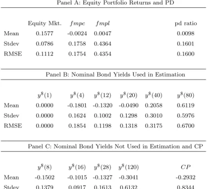
The model fits the nominal term structure of interest rates reasonably well. We match the 3-month yield exactly. For the 5-year yield, which is part of the state vector, the average pricing error is -5 basis points (bp) per year. The annualized standard deviation of the pricing error is only 13bp, and the root mean squared error (RMSE) is 13bp. For the other four yields, the mean annual pricing errors range from -18bp to +61bp, the volatility of the pricing errors range from 10 to 60bp, and the RMSE from 12 to 67bp.16 While these pricing errors are somewhat higher than the ones produced by term-structure models, our model with only 8 parameters in the term structure block of Λ1 and especially no latent variables does a good job capturing the level and dynamics of long yields. Furthermore, most of the term structure literature prices yields of maturities up to 5 years, while we also price the 10-year and 20-year yields, because these matter for pricing long-duration assets. On the dynamics, the annual volatility of the nominal yield on the 5-year bond is 1.36% in the data and 1.29% in the model.
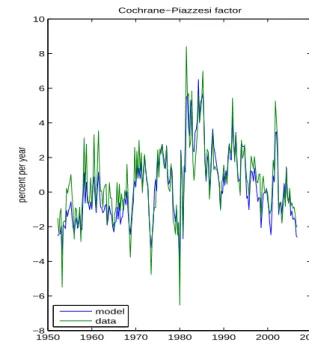
The model also does a good job capturing the bond risk premium dynamics. The model produces a nice fit between the Cochrane-Piazzesi factor in model and data. The right panel of Figure 1 shows the CP factor in model and data; it is a measure of the 1-year nominal bond risk premium. The annual mean pricing error is -29bp and standard deviation of the pricing error is 83bp. The left panel shows the 5-year nominal bond risk premium, defined as the difference between the 5-year yield and the average expected future short term yield averaged over the next 5 years. This long-term measure of the bond risk premium is also matched closely by the model, in large part due to the fact that the long-term and short-term bond risk premia have a correlation of 90%. The figure suggests our model is able to capture the substantial variation in bond risk premia in the data. This is important because the bond risk premium will turn out to constitute a major part of the consumption risk premium.
[Figure 1 about here.]
The model also manages to capture the dynamics of stock returns quite well. The bottom panel of Figure 2 shows that the model matches the equity risk premium that arises from the VAR 16Note that the largest errors occur on the 20-year yield, which is unavailable between 1986.IV and 1993.II. The
structure. The average equity risk premium (including Jensen term) is 6.90% per annum in the data, and 7.06% in the model. Its annual volatility is 9.54% in the data and 9.62% the model. The top panel shows the dynamics of the price-dividend ratio on the stock market. The model, where the price-dividend ratio reflects the present discounted value of future dividends, replicates the price-dividend ratio in the data quarter by quarter.
[Figure 2 about here.]
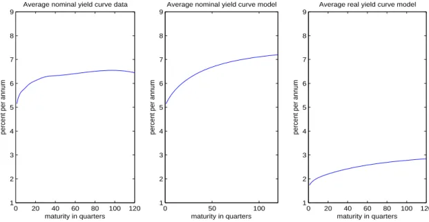
As in Ang, Bekaert, and Wei (2007), the long-term nominal risk premium on a 5-year bond is the sum of a real rate risk premium (defined the same way for real bonds as for nominal bonds) and the inflation risk premium. The right panel of Figure 3 decomposes this long-term bond risk premium (solid line) into a real rate risk premium (dashed line) and an inflation risk premium (dotted line). The real rate risk premium becomes gradually more important at longer horizons. The left panel of Figure 3 decomposes the 5-year yield into the real 5-year yield (which itself consists of the expected real short rate plus the real rate risk premium), expected inflation over the next 5-years, and the 5-year inflation risk premium. The inflationary period in the late 1970s-early 1980s was accompanied by high inflation expectations and an increase in the inflation risk premium, but also by a substantial increase in the 5-year real yield.17 Separately identifying real rate risk and inflation risk based on term structure data alone is challenging.18 We do not have long enough data for real bond yields, but stocks are real assets that contain information about the term structure of real rates. They can help with the identification. For example, higher long real yields in the late 1970s-early 1980s lower the price-dividend ratio on stocks, which indeed was low in the late 1970s-early 1980s (top panel of Figure 2). In terms of average real yields, the dotted line in Figure 4 shows yields ranging from 1.74% per year for 1-quarter real bonds to 2.70% per year for 20-year real bonds.
[Figure 3 about here.] [Figure 4 about here.]
Finally, the model matches the expected returns on the consumption and labor income growth factor mimicking portfolios (fmp) very well. The figure is omitted to save space. The annual risk premium on the consumption growth fmp is 0.79% with a volatility of 1.67 in data and model. 17Inflation expectations in our VAR model have a correlation of 80% with inflation expectations from the Survey
of Professional Forecasters (SPF) over the common sample 1981-2006. The 1-quarter ahead inflation forecast error series for the SPF and the VAR have a correlation of 68%. Realized inflation fell sharply in the first quarter of 1981. Neither the professional forecasters nor the VAR anticipated this decline, leading to a high realized real yield. The VAR expectations caught up more quickly than the SPF expectations, but by the end of 1981, both inflation expectations were identical.
18Many standard term structure models have a likelihood function with two local maxima with respect to the
Likewise, the risk premium on the labor income growth fmp is 3.87% in data and model, with volatilities of 1.92 and 1.98%.
To summarize, table 1 provides a detailed overview of the pricing errors on all these assets. Panel A shows the pricing errors on the equity portfolios, Panels B and C the pricing errors on nominal bonds. Panel A shows that the equity risk premium is 16 basis points per year lower in the data than in the model, while the factor mimicking portfolio returns have the same mean. The volatility and RMSE of the pricing errors on the equity risk premium are about 10 basis points per year. Those on the factor mimicking portfolio returns are 18 and 44 basis points, respectively. Panel B shows the pricing errors on nominal bonds that were used in estimation. The three month rate is matched perfectly since it is in the state vector and carries no risk price. The pricing error on the 5-year bond is only 5 basis points on average, with a standard deviation and RMSE of about 13 basis points. Two- and three-year bonds have pricing error volatilities of 16 and 10 basis points per year. The seven-year bond has a RMSE of 17 basis points, the ten-year bond one of 32 basis points. The largest pricing errors occur on bonds of 20- and 30-year maturity. One mitigating factor is that these bonds have some missing data over our sample period, which makes the comparison of yields in model and data somewhat harder to interpret. Another is that there may be liquidity effects at the long end of the yield curve that are not captured by our model (see Vayanos and Vila (2007)). The pricing errors for nominal bond yields that we obtain are larger than in the standard affine term structure literature, which exclusively focuses on the pricing of 1-year to 5-year bonds using latent factors. We jointly price bonds and stocks, use no latent state variables, and include much longer maturity bonds than what is typically done in the literature.
[Table 1 about here.]
3.2
The Wealth-Consumption Ratio
With the estimates for Λ0 and Λ1 in hand, it is straightforward to use Proposition 1 and solve for Ac
0 andAc1 from equations (6)-(7). The third column of Table 2 summarizes the key moments of the log wealth-consumption ratio obtained in quarterly data. The numbers in parentheses are small sample bootstrap standard errors, computed using the procedure described in Appendix B.9. We can directly compare the moments of the wealth-consumption ratio with those of the price-dividend ratio on equity. Thewc ratio has a volatility of 17% in the data, considerably lower than the 27% volatility of thepdm ratio. Thewcratio in the data is a persistent process; its 1-quarter (4-quarter) serial correlation is .96 (.85). This is similar to the .95 (.78) serial correlation ofpdm. The volatility of changes in the wealth consumption ratio is 4.86%, and because of the low volatility of aggregate consumption growth changes, this translates into a volatility of the total wealth return on the same order of magnitude (4.93%). The corresponding annual volatility of 9.8% is much lower than the 16.7% volatility of stock returns. The change in the wc ratio and the total wealth return have
weak autocorrelation (-.11 and -.01 at the 1 and 4 quarter horizons for both), suggesting that total wealth returns are hard to forecast by their own lags. The correlation between the total wealth return and consumption growth is mildly positive (.19).
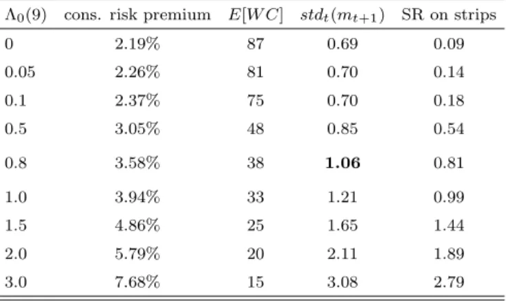
How risky is total wealth compared to equity? According to our estimation, the consumption risk premium (calculated from equation 10) is 54 basis points per quarter or 2.17% per year. This results in a mean wealth-consumption ratio (Ac
0) of 5.86 in logs, or 87 in annual levels (exp{Ac0− log(4)}). The consumption risk premium is only one-third as big as the equity risk premium of 6.9%. Correspondingly, the wealth-consumption ratio is much higher than the price-dividend ratio on equity: 87 versus 27. A simple back-of-the-envelope Gordon growth model calculation sheds light on the level of the wealth-consumption ratio. The discount rate on the consumption claim is 3.49% per year (a consumption risk premium of 2.17% plus a risk-free rate of 1.74% minus a Jensen term of 0.42%) and its cash-flow growth rate is 2.34%: 87 = 1/(.0349−.0234). Finally, the volatility of the consumption risk premium is 3.3% per year, one-third of the volatility of the equity risk premium. The standard errors on the moments of the wealth-consumption ratio or total wealth return are sufficiently small so that the corresponding moments of the price-dividend ratio or stock returns are outside the 95% confidence interval of the former. The main conclusion of our measurement exercise is that total wealth is (economically and statistically) significantly less risky than equity.
[Table 2 about here.]
If equity is one natural benchmark for the consumption claim, then the consumption perpetuity is the other natural benchmark. We recall that in the special case of i.i.d. consumption growth and zero risk prices for current and future consumption innovations, the consumption risk premium equals the risk premium on the consumption perpetuity. Table 3 reports the same moments as Table 2 but for the consumption perpetuity. We estimate a risk premium on the perpetuity of 46 basis points per quarter or 1.84% per annum. The difference with the consumption risk premium is positive but small: 33bp per year. Hence, the market assigns a small risk price to current and future consumption innovations. Almost all of the 33bp spread is due to the pricing of innovations to future consumption growth. If consumption is a random walk, the annual consumption risk premium is only 2bp above the perpetuity risk premium. Second, the price-dividend ratio on the perpetuity is less volatile than the wealth-consumption ratio (16% versus 22%). The average log wealth-consumption ratio on the perpetuity Ac,tr0 is 6.17, compared to 5.86 for the claim to actual consumption, Ac
0. This implies that the growing real perpetuity trades at a 31% premium (̟ ≃ Ac,tr0 −Ac
0 = 6.17−5.86) on average relative to the consumption claim. On average, the marginal cost of business cycles ̟ is 31% per annum, about twice as high as the benchmark estimate in Alvarez and Jermann (2004), yet much smaller than the costs predicted by the leading representative agent asset pricing models discussed below.
To further understand the source of the small difference between the prices of the consumption claim and the consumption perpetuity, we estimate a simpler bonds only version of the model in Section 5.3. This model only matches the bond-market moments by choosing the bond risk prices in the first block of Λ0 and Λ1. All other risk prices are set to zero. This simplified model delivers very similar results to our benchmark. This suggests that the small difference between the consumption risk premium and the consumption perpetuity risk premium is driven by current consumption innovations spanned by bond returns, not stock returns, or future consumption innovations driven by bond variables that predict consumption growth, not by stock returns or the dividend-price ratio.
[Table 3 about here.]
Figure 5 plots the time-series for the annual wealth-consumption ratio, expressed in levels. Its dynamics are to a large extent inversely related to the long real yield dynamics (dashed line in the left panel of Figure 3). For example, the 5-year real yield increases from 2.7% per annum in 1979.I to 7.3% in 1981.III while the wealth-consumption ratio falls from 77 to 46. This corresponds to a loss of $533,000 in real per capita wealth in 2006 dollars.19 Similarly, the low-frequency decline of the real yield in the twenty-five years after 1981 corresponds to a gradual rise in the wealth-consumption ratio. One striking way to see that total wealth behaves differently from equity is to study it during periods of large stock market declines. During the periods 1973.III-1974.IV and 2000.I-2002.IV, for example, the change in US households’ real per capita stock market wealth, including mutual fund holdings, was -46% and -61%, respectively. In contrast, real per capita total wealth changed by -12% and +27%, respectively. Over the full sample, the total wealth return has a correlation of only 12% with the value-weighted real CRSP stock return, while it has a correlation of 46% with realized one-year holding period returns on the 5-year nominal government bond.20 Likewise, the (1-period) consumption risk premium has a correlation of 22% with the (1-period) equity risk premium, but 66% with the (1-period) nominal bond risk premium.
[Figure 5 about here.]
To show more formally that the consumption claim behaves like a real bond, we compute the discount rate that makes the current wealth-consumption ratio equal to the expected present discounted value of future consumption growth (See Appendix C.2 for details). This is the solid line measured against the left axis of Figure 6. Similarly, we calculate a time series for the discount rate on the dividend claim, the dotted line measured against the right axis. For comparison, we plot the 19Real per capita wealth is the product of the wealth-consumption ratio and observed real per capita consumption. 20A similarly low correlation of 12% is found between total wealth returns and the Flow of Fund’s measure of
the growth rate in real per capita household net worth, a broad measure of financial wealth. The correlation of the total wealth return with the Flow of Fund’s growth rate of real per capita housing wealth is 0.11.
yield on a long-term real bond (50-year) as the dashed line against the right axis. The correlation between the consumption discount rate and the real yield is 99%, whereas the correlation of the dividend discount rate and the real yield is only 44%. In addition, the consumption and dividend discount rates only have a correlation of 47%, reinforcing our conclusion that the data suggest a large divergence between the perceived riskiness of a claim to consumption and a claim to dividends in securities markets.
[Figure 6 about here.]
Consumption Strips A different way of showing that the consumption claim is bond-like is to study yields on consumption strips. It is useful to decompose the yield on the period-τ strip in two pieces. The first component is the yield on a security that pays a certain cash flow (1 +µc)τ. The underlying security is a real perpetuity with a certain cash flow which grows at a deterministic consumption growth rate µc. The second component is the yield on a security that pays off Cτ/C0−(1 +µc)τ. It captures pure consumption cash flow risk. Appendix B.5 shows that the log price-dividend ratios on the consumption strips are affine in the state, and details how to compute the yield on its two components. Figure 7 makes clear that the consumption strip yields are mostly comprised of a compensation for time value of money, not consumption cash flow risk.
[Figure 7 about here.]
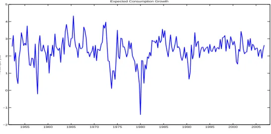
Potential Limitations Our consumption risk premium estimates could be too low (i) if there is some variable we omitted that predicts consumption growth and carries a positive price of risk, (ii) if we mis-measured the covariance between aggregate consumption growth and the state variables, or (iii) if consumption innovations that are not spanned, are priced. In case (i), we mis-measure the price assigned to innovations to future consumption growth by our model. While we cannot rule out that our VAR misses some predictability of consumption growth at longer horizons, the literature has found modest statistical evidence for consumption growth predictability. Our VAR contains the variables that have been shown to have some predictability: the yield spread, the short-term interest rate, and the price-dividend ratio on the stock market. Our state variables zt explain 19% of variation in ∆ct+1 in our benchmark quarterly exercise and even 40% at annual frequency (see Section 5.4). Figure 8 plots the (annualized) one-quarter-ahead expected consumption growth series implied by our VAR. The volatility of annualized expected consumption growth is 0.37% (more than one-third of the volatility of realized consumption growth), while the first-order autocorrelation of expected consumption growth is 0.54 in quarterly data. Moreover, as is clear from the figure, expected consumption growth experiences the largest declines during the severe NBER recessions in the first part of the sample, the 1953.II-1954.II recession, the 1957.III-1958.II recession, the 1973.IV-1975.I recession, the double-dip NBER recession from 1980.I to 1982.IV, and somewhat