published 11 February 2020)
Digital rock imaging plays an important role in studying the microstructure and macroscopic properties of rocks, where microcomputed tomography (MCT) is widely used. Due to the inherent limitations of MCT, a balance should be made between the field of view (FOV) and resolution of rock MCT images—a large FOV at low resolution (LR) or a small FOV at high resolution (HR). However, large FOV and HR are both expected for reliable analysis results in practice. Super-resolution (SR) is an effective solution to break through the mutual restriction between the FOV and resolution of rock MCT images, for it can reconstruct an HR image from a LR observation. Most of the existing SR methods cannot produce satisfactory HR results on real-world rock MCT images. One of the main reasons for this is that paired images are usually needed to learn the relationship between LR and HR rock images. However, it is challenging to collect such a dataset in a real scenario. Meanwhile, the simulated datasets may be unable to accurately reflect the model in actual applications. To address these problems, we propose a cycle-consistent generative adversarial network (CycleGAN)-based SR approach for real-world rock MCT images, namely, SRCycleGAN. In the off-line training phase, a set of unpaired rock MCT images is used to train the proposed SRCycleGAN, which can model the mapping between rock MCT images at different resolutions. In the on-line testing phase, the resolution of the LR input is enhanced via the learned mapping by SRCycleGAN. Experimental results show that the proposed SRCycleGAN can greatly improve the quality of simulated and real-world rock MCT images. The HR images reconstructed by SRCycleGAN show good agreement with the targets in terms of both the visual quality and the statistical parameters, including the porosity, the local porosity distribution, the two-point correlation function, the lineal-path function, the two-point cluster function, the chord-length distribution function, and the pore size distribution. Large FOV and HR rock MCT images can be obtained with the help of SRCycleGAN. Hence, this work makes it possible to generate HR rock MCT images that exceed the limitations of imaging systems on FOV and resolution.
DOI:10.1103/PhysRevE.101.023305
I. INTRODUCTION
X-ray microcomputed tomography (MCT) is a widely used imaging technology to obtain three-dimensional (3D) images of porous media, such as rock, soil, wood, and ceramic. For digital rock imaging, MCT plays an important role. The 3D images produced by MCT show the microstructures of rock samples and therefore can be used to analyze the macroscopic properties of rocks, such as permeability and conductivity [1–4]. To obtain reliable analysis results, rock MCT images with high resolution (HR) and a large field of view (FOV) are desired. However, this is challenging in practice because of the inherent limitations of MCT. More specifically, a trade-off should be made between the FOV and resolution of MCT
†Corresponding author: [email protected] ‡[email protected]
§[email protected] [email protected] ¶[email protected]
images [5,6]. Actually, rock MCT images with a large FOV are typically of low resolution (LR), which causes increased difficulty of property analysis as many fine structures (e.g., pores) cannot be captured. On the contrary, HR images are usually with a small FOV, thereby resulting in decreased representativeness. Recent studies [7–11] show that this bot-tleneck can be addressed to some extent via super-resolution (SR), which maps a LR input to a space of higher resolution [12]. HR rock MCT images with a large FOV can be obtained by applying SR algorithms to the collected LR MCT images.
SR is an active research direction in the image and video processing area and extensive studies [13–45] have been done on this topic in recent years. Existing SR methods can be roughly classified into the following categories based on the object: Single image SR [13–40], multiframe SR [41,42], and video SR [43–45]. Single image SR refers to the reconstruc-tion of an image with higher resolureconstruc-tion from a single LR observation. For multiframe SR, a set of correlated LR images is used as the input to estimate an HR image. Correspondingly, video SR aims to produce an HR video from the acquired LR video. Overall, single image SR has received greater attention among the three groups for it is more practical in
most cases. Traditional single image SR methods [13–19] usually combine the imaging model of LR observations and the prior knowledge of HR images to formulate an objective function, which is optimized to produce an HR estimate. Commonly used priors include sparsity [13], local smoothness [14], nonlocal similarity [15], low rank [17,18], gradient information [18,19], etc. Learning-based single image SR approaches [20–40] have become mainstream in recent years. This kind of approach learns the mapping between LR-HR image pairs in the model training stage, and LR test images are super-resolved using the learned mapping in the testing phase. Neighbor embedding [20], sparse representation [21], neighbor regression [22,23], random forest [24], and deep neural networks [25–40] are effective models for character-izing the mapping from LR to HR images. In particular, deep convolutional neural networks (CNNs) have shown excellent performance on a variety of computer vision tasks [46–59], and SR is no exception. Therefore, this work mainly focuses on deep CNN-based single image SR approaches.
The super-resolution convolutional neural network (SRCNN) proposed by Dong et al. [25] is one of the representative works for deep CNN-based SR algorithms. SRCNN consists of three convolutional layers, which perform block extraction, mapping, and reconstruction, respectively. SRCNN achieved state-of-the-art performance when first proposed, although its structure is simple. Subsequently, several of the networks were developed for single image SR. Typically, a deconvolutional layer used for upsampling was incorporated into the fast super-resolution convolutional neural network (FSRCNN) [26]. Shiet al. [27] developed a subpixel layer to produce the HR output from LR features. The deconvolutional layer and the subpixel layer were widely used in subsequent studies [32–34] because they are helpful for improving efficiency. Kim et al. [28] presented a very deep (20 layers) SR network (VDSR) using residual learning and gradient clipping. This work shows that within a certain
range, the quality of the super-resolved result improves as the network depth increases. Overall, follow-up networks for SR became deeper and deeper. In order to avoid excessive parameters of deep neural networks, recursive structures were used in the deeply-recursive convolutional network (DRCN) [29] and the deep recursive residual network (DRRN) [30]. Limet al.[31] greatly improved the model capacity via en-hancing network depth and width, and the designed enhanced deep residual network for SR (EDSR) won the New Trends in Image Restoration and Enhancement (NTIRE) challenge 2017 [60]. Zhanget al.[33] combined the dense block and the resid-ual block, and presented a deep residresid-ual dense network (RDN) for single image SR. Subsequently, the authors developed a deep residual channel attention network (RCAN, over 400 layers) for SR via combining the residual in residual structure and the channel attention mechanism [34]. The methods mentioned above focus more on the objective parameters [e.g., peak signal-to-noise ratio (PSNR) and structural similarity index (SSIM)] of the recovered HR images. RDN [33] and RCAN [34] are state-of-the-art approaches in terms of PSNR and SSIM. However, these indexes may not be consistent with the human visual system in some cases. To address this problem, a series of perceptual-driven SR approaches [35–40] have been presented. The pioneer of this kind of algorithm is the generative adversarial network-based SR method (SRGAN) [35]. Aiming to improve the visual quality of the HR estimate, SRGAN was trained with perceptual and adversarial losses. The loss functions for network training affect SR performance greatly. Hence, a variety of losses were designed, including the local texture matching loss [36] and the contextual loss [37]. Parket al.[38] introduced an additional discriminator into a GAN-based SR network to produce more realistic results. Yuan et al. [39] and You et al. [40] developed unsupervised and semisupervised SR frameworks using the cycle-consistent generative adversarial network (CycleGAN) [61]. Overall, compared with objective
FIG. 1. Examples of unpaired and paired LR-HR images. (a) Unpaired LR-HR images in the real world. (b) Paired LR-HR images produced by simulation. Please zoom in to view details and make comparisons.
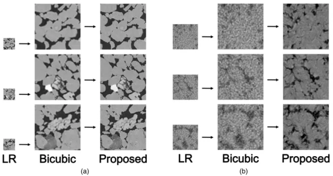
FIG. 2. Examples of rock MCT images SR. (a) Results on simulated LR images (SR factor: 4×; from left to right: LR, bicubic interpolation, proposed SRCycleGAN). (b) Results on real-world LR images (SR factor: 1.8×; from left to right: LR, bicubic interpolation, proposed SRCycleGAN). Please zoom in to view details and make comparisons.
parameters-driven SR methods, perceptual-driven approaches can produce visually more pleasant HR images.
With the rapid development of SR, the SR of rock MCT images is attracting more and more attention for its significant application potential in digital rock imaging. Wanget al.[7] improved the resolution of MCT images of rock samples using neighbor embedding. For the reconstructed HR rock image, the low-frequency part is provided by the LR MCT input, and the HR scanning electron microscopy (SEM) provides high-frequency information. Wang et al. [8,9] trained a set of networks including SRCNN, EDSR, and SRGAN for rock MCT images SR. There are also some studies for the SR of 3D rock images. For example, Liet al.[10] presented a sparse representation-based 3D volumetric SR framework. Wang et al.[11] extended the VDSR for 3D rock MCT images SR via introducing 3D convolution. These studies demonstrate that the resolution of rock MCT images can be enhanced by performing SR.
To the best of our knowledge, paired LR-HR training images are necessary for most of the existing learning-based SR approaches for rock MCT images [7–11]. However, it is challenging to collect paired LR-HR images of the same rock sample in a real scenario. Even though we can scan the same sample using different devices to generate images with different resolutions [as shown in Fig. 1(a)], accurate registration between images is very difficult. One solution for this problem is to produce LR-HR image pairs artificially [as shown in Fig.1(b)]. Given an HR rock image, the cor-responding LR image can be generated by downsampling. Producing accurately paired LR-HR images is convenient and efficient in this way. However, the relationship between simulated LR-HR image pairs may not reflect the actual mapping because the real-world LR images usually suffer from more complex degradations (nonideal blur, sensor noise,
compression artifacts, etc.), resulting in poor SR performance in practical applications.
This paper proposes an effective SR approach for real-world rock MCT images, namely, SRCycleGAN. Some SR results both on the simulated and real-world LR rock MCT images are illustrated in Fig. 2. It can be observed that the super-resolved results by the proposed SRCycleGAN are much better than LR images as well as the results of bicubic interpolation, with more details and clearer edges. Apparently, the SR process would be helpful for subsequent process and analysis. The main contributions of this work are as follows:
(1) To overcome the absence of paired training examples, we propose to consider the SR of real-world rock MCT images as the unpaired image-to-image translation. LR rock images and the associated HR rock images are assumed to belong to two related domains.
(2) We present a CycleGAN-based SR approach that is well suited to the SR of real-world rock MCT im-ages, where paired LR-HR training images are difficult to obtain.
(3) Extensive experiments are performed to demonstrate the effectiveness and superiority of the proposed SRCycle-GAN. In particular, a set of statistical parameters is compared between the SR results and targets to validate the reliability of SRCycleGAN.
(4) This work shows that, with an effective SR method, the inherent hardware limitations of digital rock imaging systems on the FOV and resolution can be compensated to some extent.
The remainder of this paper is organized as follows. Section II presents the proposed SRCycleGAN in detail. Experimental results and discussion are shown in Sec. III. SectionIVconcludes this study.
FIG. 3. The architecture of CycleGAN [61]. (a) CycleGAN comprises two generators (GX :Y →Xand GY :X →Y) and two associated discriminators (DX andDY). (b) Forward cycle consistency:x≈GX(GY(x)). (c) Backward cycle consistency:y≈GY(GX(y)).
II. SRCycleGAN: CycleGAN-BASED SR ALGORITHM FOR REAL-WORLD ROCK MCT IMAGES
A. Motivation
To address the problem of the mismatch between LR and HR training images (unpaired data), we propose to use CycleGAN [61] to learn the mapping between LR and HR images for the following reasons:
(1) Although it is difficult to obtain exactly matched LR-HR rock MCT images in a real scenario, collecting the images of the same sample at different resolutions is feasible. There-fore, unpaired LR-HR images of the same rock sample (or similar rock samples) can be obtained.
(2) CycleGAN is particularly suitable for translating the input from a source domain X to a target domainY in the absence of paired input-output examples, making the distribu-tion of the translated results from images inX indistinguish-able from the distribution of images inY.
We assume that LR rock images and the associated HR rock images belong to two related domains, i.e., different renderings of the same underlying scene. Correspondingly, our goal is to learn the underlying relationship between the LR domain and the HR domain, which can be achieved by using CycleGAN.
It should be noted that the goal of this work is to address the conflict between the FOV and the resolution of computed tomography (CT) images in real-world applications. To be more accurate, we aim to obtain an HR CT image with a large FOV from a LR observation using SR techniques. The absence of paired LR-HR examples for SR model training is one of the biggest challenges in a real scenario. To address this problem, this work proposes to consider the SR problem as the unpaired image-to-image translation. Because the target of this work is not to develop new networks, we adopt one of the most well-known algorithms for unpaired image-to-image translation, i.e., the CycleGAN [61], as the backbone of the proposed SR method.
B. An overview of CycleGAN
Figure 3 presents the schematic diagram of CycleGAN [61], which aims to translate an image in domainXto a target domainY given one training set of images inX and another image set inY. As shown in Fig. 3(a), CycleGAN consists of two generators (i.e., GX and GY) and two adversarial
discriminators (i.e.,DX andDY). GX, GY, DX, and DY are
deep neural networks. Specifically,GX models the mapping
Y →X, such that the translated image ˆx=GX(y), y∈Y,
is indistinguishable from images x∈X by the associated discriminator DX. DX is trained to distinguish ˆx (generated
data in the X domain) fromx (real data in the X domain). GY is the inverse ofGX; i.e., it learns the relationshipX →
Y, making the output ˆy=GY(x), x∈X, similar to images
y∈Y in the view of DY.DY aims to distinguish between ˆy
and y. The cycle-consistency property shown in Figs. 3(b)
and 3(c) is one of the main characteristics of CycleGAN, which can guarantee the consistency between GX and GY,
i.e., GX(GY(x))≈x [forward cycle consistency, Fig. 3(b)]
andGY(GX(y))≈y[backward cycle consistency, Fig.3(c)].
Inspired by the impressive performance of CycleGAN on unpaired image-to-image translation, we take it as a backbone to develop the SR method for real-world rock MCT images in this work.
C. Proposed method
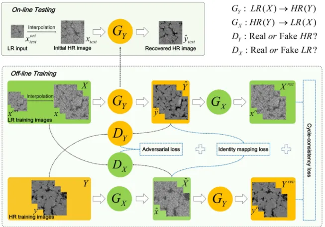
Figure 4 illustrates the framework of the proposed CycleGAN-based SR method for real-world rock MCT im-ages, namely, SRCycleGAN, which consists of two stages: Off-line training (bottom) and on-line testing (top).GY aims
to translate LR rock images from domain X into an image domain Y of higher resolution against DY that attempts to
distinguish real and fake HR images. Meanwhile, GX tries
to produce LR rock images that belong to the LR domain X against DX that differentiates fake LR images from real
samples inX.
1. Off-line training
Without loss of generality, we denote LR and HR train-ing samples as {xi}P
i=1 (xi∈X and xi∈RM×N) and {yj} Q j=1 (yj ∈Y andyj∈RM×N), respectively. It is important to note
that, as shown in Fig.4, the original LR training images are upsampled to the expected resolution before being fed into the network. More specifically, LR training samples{xi}Pi=1, which have the same resolution (i.e.,M×N) as HR training samples {yj}Qj=1, are the upscaled results of the original LR images {xori i } P i=1 (xiori∈R M s× N
s), wheresdenotes the
upsam-pling factor. Although upsamupsam-pling results {xi}Pi=1 (xi∈X)
have the same size as expected, we still call them LR training images for low quality.
Unpaired LR and HR rock images {xi}Pi=1, {yj}
Q j=1 are used to train the four networks GX, GY, DX, and DY in
FIG. 4. The off-line training phase (bottom) and the on-line testing phase (top) of the proposed SRCycleGAN.
SRCycleGAN following the objective
L(GX,GY,DX,DY,X,Y)
=λ1Lgan(GX,DX,GY,DY,X,Y) +λ2Lcyc(GX,GY,X,Y)
+λ3Lide(GX,GY,X,Y), (1)
where Lgan, Lcyc, and Lide represent the adversarial loss, the cycle-consistency loss, and the identity mapping loss, respectively. λ1, λ2, and λ3 are used to adjust the relative importance of the three terms on the right-hand side. Three loss functions are detailed in the following.
The adversarial loss Lgan makes the distribution of the translated data ( ˆxand ˆy) accord with the distribution of the data (x andy) in the target domain (X andY). To be more specific, GY (GX) tries to produce HR (LR) rock images
that look like real HR (LR) images in domainY (X). The generated HR (LR) results by generator GY (GX) should
be indistinguishable from real HR (LR) rock images for the corresponding discriminator DY (DX). The objective is
formulated as
Lgan(GX,DX,GY,DY,X,Y)
=LganX(GX,DX,X,Y)+LganY(GY,DY,Y,X), (2)
where LganX(GX,DX,X,Y)=Ex∼pdata(x)[logDX(x)]+ Ey∼pdata(y)[log(1−DX(GX(y)))] and LganY(GY,DY,Y,X)= Ey∼pdata(y)[logDY(y)]+Ex∼pdata(x)[log(1−DY(GY(x)))]. x∼ pdata(x) andy∼pdata(y) denote the distribution of LR and HR rock samples, respectively. TakingLganX(GX,DX,X,Y) as an
example, GX aims to produce a LR rock image ˆx=GX(y)
that looks like images in the LR domain X, whileDX tries
to make a distinction between the translated result ˆxand real LR samples inX. Mathematically,GX attempts to minimize LganX(GX,DX,X,Y) against DX that aims to maximize
the same objective, i.e., min
GX maxDX LganX(GX,DX,X,Y). The LganY(GY,DY,Y,X) for generator GY and its discriminator
DY is similar toLganX(GX,DX,X,Y).
The cycle-consistency lossLcycencourages the two gener-ators (GX andGY) to be inverse of each other. As presented
in Fig. 4, for each LR rock image x in X, GX should be
able to bring the translated HR rock image ˆy=GY(x) back to
the original one, i.e., xrec=GX(GY(x))≈x. This constraint
is calledforward cycle consistency. Similarly, thebackward cycle consistency is defined as yrec=G
Y(GX(y))≈y. The
cycle consistency is achieved using the following loss:
Lcyc(GX,GY,X,Y)=Ex∼pdata(x)[GX(GY(x))−x1]
+ Ey∼pdata(y)[GY(GX(y))−y1]. (3)
The identity mapping loss Lide constrains the two gen-erators (GX and GY) to manifest as an identity mapping
when the images from the target domain are used as the input. Specifically, GX (GY) is expected to output the input
when feeding LR (HR) rock images, i.e., GX(x)≈x and
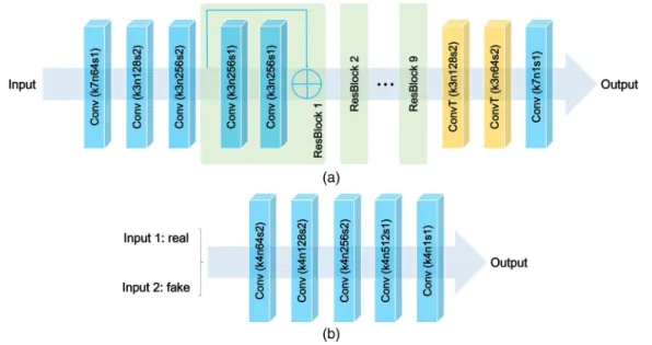
FIG. 5. Network architecture. (a) The architecture of generators (GX andGY). (b) The architecture of discriminators (DX andDY). Conv, convolutional layer; ConvT, deconvolutional layer. For each convolutional layer and deconvolutional layer, the numbers after symbols “k,” “n,” and “s” denote kernel size, number of kernels, and stride size, respectively. Note that nonlinear activation layers and normalization layers are omitted for simplicity.
loss:
Lide(GX,GY,X,Y)=Ex∼pdata(x)[GX(x)−x1]
+ Ey∼pdata(y)[GY(y)−y1]. (4) Summarizing the above, the two generators (GX andGY)
and two discriminators (DX and DY) can be optimized via
solving GX∗,GY∗,DX∗,DY∗ =arg min GX,GY max DX,DY L(GX,GY,DX,DY,X,Y). (5)
Although four subnetworks in Eq. (5) are jointly optimized in the off-line training phase, onlyGYthat can translate LR rock
images into HR images is used at the on-line testing stage. 2. On-line testing
Given a LR rock imagextestori ∈Rm×n, as presented in Fig.4, we first upsample it to the expected resolution (ms×ns) using a simple interpolation method, like bicubic. The upsampling result is denoted asxtest∈Rms×ns. The learned generatorGY
is applied toxtestto produce an HR rock image ˆytest∈Rms×ns as
ˆ
yt est =GY(xt est). (6)
D. Network architecture
Figure 5 shows the architectures of generators GX, GY
and discriminatorsDX,DY. Note that only major components
are presented, omitting nonlinear activation layers and nor-malization layers for simplicity. In Fig.5, the convolutional layers and deconvolutional layers are expressed as “Conv” and “ConvT,” respectively. For each convolutional layer and deconvolutional layer, the numbers after symbols “k,” “n,” and “s” represent kernel size, number of filters, and stride size, respectively. For example, “Conv (k3n128s2)” represents a
convolutional layer that contains 128 filters, and the filter size is 3×3 and the stride is set to 2.
The two generatorsGX andGY in Fig.4 share the same
architecture, as shown in Fig.5(a). The network illustrated in Fig. 5(a)consists of three parts. The first part is composed of three convolutional layers that gradually reduce feature size and increase the channel of features. And an activation layer is placed after each convolutional layer. The second part contains nine residual blocks, and each of then is composed of two convolutional layers and an activation layer in the middle. For the third part, two deconvolutional layers are adopted to increase feature size while decreasing the channel of features first, and then the last convolutional layer transforms features into the expected number of the output channel. The detailed settings of these convolutional and deconvolutional layers are indicated in the figure.
The two discriminatorsDX andDY in Fig.4also share the
same architecture, as presented in Fig.5(b). The discriminator contains five convolutional layers, which are followed by an activation layer except for the last one. The first three layers increase the channel of features while reducing feature size, and the fourth layer further increases the number of feature channels to 512. The last convolutional layer compresses its input into one channel.
E. Datasets and training details
To more comprehensively test the ability of the proposed SR method for rock MCT images, SRCycleGAN is trained and tested on three datasets, i.e.,Sandstone_Real_1.8x, Sand-stone_SiDe_4.0x, andSandstone_SiUn_4.0x.
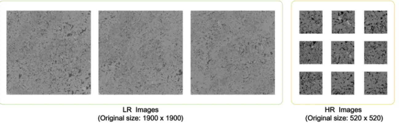
a. Sandstone_Real_1.8x. This is a dataset we have built, which contains unpaired LR–HR rock MCT images of the same sandstone sample. HR rock images are imaged at a resolution of 5μm and LR rock images are imaged at 9μm. This dataset is composed of 900 LR images of size 1900× 1900 and 512 HR images of size 520×520. Figure6presents
FIG. 6. Visualization of LR and HR images in the proposed datasetSandstone_Real_1.8x. Please zoom in to view details and make comparisons.
some examples of this dataset. 2048 subimages (256×256) extracted from HR rock images are used as HR samples for network training. LR rock images are 1.8×upsampled first to a resolution at 5μm, and then 22 000 subimages (256×256) cropped from the interpolated LR images are used as LR samples for model training (20 000 images) and testing (2000 images). Note that there is no overlap between the LR samples for training and testing.
b. Sandstone_SiDe_4.0x.This dataset is provided by Wang et al.[62]. The size of 800 HR rock images in this dataset is 800×800. These HR images are 4× downsampled to generate matched LR rock images using the imresize function
inMATLAB, and the interpolation kernel is set to “bicubic.”
Hence, LR images are 200×200. In our experiments, 7200 HR samples (256×256) are extracted from HR rock images for network training. LR rock images are first 4×upsampled to the size of 800×800, and 12 000 subimages (256×256) cropped from the interpolated LR images are used as LR samples for network training. It is important to note that although paired HR-LR rock images can be obtained for this dataset, we do not use paired data for network training. The extracted HR and LR training samples are not matched. Wang et al.[62] also provided a corresponding testing dataset, which contains 100 LR images (200×200) and their ground truth. We crop 9 subimages from each upscaled LR image (900 subimages in total) for testing, and 900 HR counterparts are cropped from the ground truth for performance evaluation. Similarly, there is no overlap between the LR samples for training and testing.
c. Sandstone_SiUn_4.0x. This dataset provided by Wang et al.[62] is almost the same asSandstone_SiDe_4.0x, except a randomly selected interpolation kernel (including “box,” “triangle,” “cubic,” “lanczos2,” and “lanczos3”) is applied to each HR image for downsampling. For this dataset, we use the same strategy asSandstone_SiUn_4.0xto extract HR and LR training and testing samples.
We use PyTorch for training and testing on an NVIDIA GeForce GTX 1080Ti GPU. The Adam solver [63] is used to optimize our network SRCycleGAN with a batch size 1. All models are trained for 50 epochs from scratch with the initial learning rate 0.0002. The learning rate for the first 25 epochs is set to 0.0002 and it linearly decays to zero over the next 25 epochs.λ1,λ2, and λ3 in Eq. (1) are set to 1, 10, and 5, respectively [64].
III. RESULTS AND DISCUSSION A. Performance evaluation criteria
Objective and subjective comparisons are combined to evaluate the performance of the proposed SR approach SR-CycleGAN.
For the experiments on simulated LR rock images from Sandstone_SiDe_4.0xandSandstone_SiUn_4.0x, in addition to visual effect comparisons, the PSNR is used to quantita-tively assess the quality of the reconstructed HR rock images for the HR ground truth of each LR test image available. The PSNR is a full-reference image quality assessment index that measures the difference between two images by a comparison of pixel values [65]. PSNR is widely used for SR performance evaluation [9,11,33], and it is defined as
PSNR=10log10 2552 MSE, (7) MSE= 1 HW H i=1 W j=1 [Iref(i,j)−I(i,j)]2,
where I∈RH×W and Iref ∈RH×W denote the recovered im-age and the corresponding ground truth, respectively. Gener-ally, higher PSNR scores indicate better SR performance.
For the experiments on real-world rock MCT images, we first present the visual quality of the recovered HR images, and then quantitatively measure the accuracy and reliability of these results using a set of evaluation parameters.
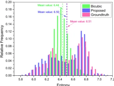
Since there are no LR-HR image pairs in this test, the entropy is used to quantitatively evaluate the results produced by bicubic interpolation and our method SRCycleGAN. The entropy is a no-reference quality assessment index that mea-sures the uncertainty, localization, and concentration [66]. The definition of the entropy is
Entropy= −
L−1
i=0
pilog2pi, (8)
where pirepresents the probability density function of theith
gray level, andLdenotes the number of gray levels.
In addition, the porosity [67], the local porosity distribution [67,68], the two-point correlation function [2], the lineal-path function [69], the two-point cluster function [70], the chord-length distribution function [71], and the pore size distribution
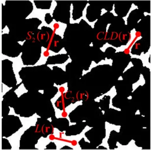
FIG. 7. Illustration of the two-point correlation functionS2(r),
the lineal-path functionL(r), the two-point cluster functionC2(r),
and the chord-length distribution functionCLD(r). The white part denotes the phase of interest and the black part is background.
[72] are employed to evaluate the consistency between the binarization results of the reconstructed HR rock images and the referred HR images (i.e., HR training images) from different perspectives. It should be noted that these parameters have been widely used to evaluate the performance of the algorithms for porous media reconstruction [3,4,47,59,73]. For two-dimensional images, the porosity refers to the ratio between the area of the pores and the sample area [67]. The local porosity distribution presents the probabilities of differ-ent local porosity values [67,68], and it can provide valuable information for measuring the physical properties (e.g., the permeability and diffusion quality) of porous media. Figure7
illustrates the definitions of four morphological functions on a binary image. Given a line of lengthr= r, the two-point correlation functionS2(r) denotes the probability that the two endpoints of the line lie in the same phase [2]. Similarly, the two-point cluster functionC2(r) represents the probability that the two endpoints are in the same cluster [70]. The lineal-path functionL(r) represents the probability that the line is located entirely within the same phase [69]. The chord-length distribution function CLD(r) is an important index that measures the shape and size distribution of microscale constituents [71]. As shown in Fig.7, a chord refers to a line segment whose midpoints are wholly in the phase of interest and endpoints are situated in the juncture of different phases. The pore size distribution PRDis also used as an index to measure the consistency between the recovered HR images and the ground truth [72]. In our experiments, the pores of different shapes are simplified in the shape of circles while calculating the pore radius. Mathematically, the pore radiusr is defined as√A/π, whereAdenotes the area of a pore.
B. Experiments on simulated LR rock MCT images
We first conduct experiments on simulated LR rock MCT images for more intuitive and more accurate comparisons
between the reconstructed HR rock images and the corre-sponding ground truth. It should be noted that each LR testing image has an HR counterpart in this simulation experiment. Therefore, both qualitative and quantitative comparisons be-tween the SR results and the real HR images can be conducted to evaluate the performance of the proposed SR method. As previously mentioned, 900 LR rock MCT images from Sandstone_SiDe_4.0x and 900 from Sandstone_SiUn_4.0x are used in this test, and the SR factor is set to 4. Figures8
and9present some examples of the recovered HR rock images and the ground truth counterparts. Specifically, Fig.8shows the results on Sandstone_SiDe_4.0x and Fig. 9 shows the results on Sandstone_SiUn_4.0x. It can be observed from Figs. 8 and9 that the resolution of the input (the first row) is so low that small structures are imperceptible. Although the results produced by bicubic interpolation (the second row) are larger than the corresponding inputs, they are blurred to some extent, especially in the areas of edges and textures. The HR rock images generated by the proposed SRCycleGAN (the third row), by contrast, not only have higher spatial resolution but also contain clearer edges and richer details. The results by our method are more visually appealing than the images produced by bicubic interpolation. And more importantly, it can be seen from Figs. 8 and 9 that the recovered HR images by the proposed SR method are very close to the corresponding targets. Even for the LR images with multiple components (e.g., different kinds of minerals), the SR results by SRCycleGAN are in good agreement with the original HR images. These results demonstrate the effectiveness and reliability of the proposed method.
Figure 10 presents the PSNR scores achieved by bicu-bic interpolation and the proposed SRCycleGAN, which are calculated between the recovered HR rock images and the corresponding ground truth. In general, higher PSNR values indicate better SR performance because the SR results are closer to the original HR images. The distributions of PSNR scores on Sandstone_SiDe_4.0x and Sandstone_SiUn_4.0x are illustrated in Figs. 10(a)and 10(b), respectively. Over-all, the performance of the proposed SRCycleGAN is better than bicubic interpolation in terms of PSNR. The average PSNR scores achieved by the proposed method (26.34 and 26.14 dB) are higher than that of bicubic interpolation (25.95 and 25.74 dB) on both testing datasets. The PSNR gains achieved by SRCycleGAN quantitatively verify that the HR images produced by our approach are more reliable than the results by bicubic interpolation. Note that the average PSNR scores on Sandstone_SiDe_4.0x by bicubic interpo-lation and our method are about 0.2 dB higher than that onSandstone_SiUn_4.0x. The main reason is that LR train-ing and testtrain-ing images are generated in different ways for the two datasets. For Sandstone_SiDe_4.0x, HR images are downsampled to generate LR counterparts using the “imre-size” function, with the fixed interpolation kernel “bicubic.” However, forSandstone_SiUn_4.0x, a randomly selected in-terpolation kernel is applied to each HR image to generate a LR image. Clearly, the setting onSandstone_SiDe_4.0xis relatively simpler, and thus better upsampling performance can be achieved. This phenomenon shows that the degradation model (i.e., the way to generate LR images) would affect SR performance.
FIG. 8. Visual comparison for 4×SR on the testing images inSandstone_SiDe_4.0x. From top to bottom: LR rock images, the HR results produced by bicubic interpolation, the HR results produced by the proposed SRCycleGAN, and the ground truth. Please zoom in to view details and make comparisons.
The comparisons on visual quality and PSNR of the recov-ered HR images verify the effectiveness and superiority of the proposed SR framework for rock MCT images. It is important to highlight that unpaired samples are used for model training in this test, although we have LR-HR image pairs. That is, the one-to-one relationships between LR and HR training im-ages are ignored to simulate a real-world scenario. The good agreement between the SR results by SRCycleGAN and the original HR images demonstrates that the proposed method can recover a reliable HR image from a LR observation, even without paired LR-HR images for model training.
C. Experiments on real-world LR rock MCT images
This section presents the experimental results on real-world rock MCT images. Figure11compares the perceptual quality of LR images (the first row), the recovered HR rock images by bicubic interpolation (the second row), and the proposed SRCycleGAN (the third row). In this test, there are no paired HR images corresponding to the LR testing images observed in a real-world scenario. Therefore, some HR training images (denoted as “Groundtruth” in Fig.11) are shown in the fourth row for more intuitive comparisons. It is
FIG. 9. Visual comparison for 4×SR on the testing images inSandstone_SiUn_4.0x. From top to bottom: LR rock images, the HR results produced by bicubic interpolation, the HR results produced by the proposed SRCycleGAN, and the ground truth. Please zoom in to view details and make comparisons.
24.0 24.5 25.0 25.5 26.0 26.5 27.0 27.5 28.0 0.00 0.05 0.10 0.15 0.20 0.25 Relative F requency PSNR (dB) Bicubic Proposed
Mean value:25.95 dB Mean value: 26.34 dB
Bicubic Proposed 23.5 24.0 24.5 25.0 25.5 26.0 26.5 27.0 27.5 0.00 0.02 0.04 0.06 0.08 0.10 0.12 0.14 0.16 0.18 Relative Frequency PSNR (dB) Mean value: 25.74 dB Mean value: 26.14 dB (a) (b)
FIG. 10. PSNR comparison for 4×SR on simulated LR images. (a) The PSNR scores achieved by bicubic interpolation and the proposed SRCycleGAN on 900 testing images inSandstone_SiDe_4.0x. (b) The PSNR scores achieved by bicubic interpolation and the proposed SRCycleGAN on 900 testing images inSandstone_SiUn_4.0x.
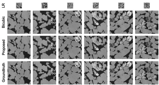
important to note that the HR images shown in the fourth row (“Groundtruth”) do not match the images in other rows. In the following figures, we use similar expressions. It can be seen that LR images and the upsampling results by bicubic interpolation suffer from a variety of artifacts, resulting in the overlapping of the pore part and the stone part. For the HR images produced by the proposed framework SRCycleGAN, they are much clearer and lots of pores are well recovered. Meanwhile, the pore part and the stone part are distinguished better, which helps the subsequent processing and analysis.
In addition, although in this test we do not have the real HR counterparts of the input as the reference, one can observe that the recovered HR rock images by the proposed SRCycleGAN are very similar to HR training images, i.e., our targets. Specifically, it can be observed from the last column of Fig.11
that there is a bright region in the HR image reconstructed by the proposed SRCycleGAN. As we understand it, there are two main reasons. First, the LR testing image in the last column contains a bright area, which can also be found in the SR result by bicubic interpolation. Second, bright areas
FIG. 11. Visual comparison for 1.8×SR on the testing images inSandstone_Real_1.8x. From top to bottom: LR rock images, the HR results produced by bicubic interpolation, the HR results produced by the proposed SRCycleGAN, and the ground truth. Note that the ground truth in this figure refers to HR training images, which do not match LR images. In the following figures, we use similar expressions. Please zoom in to view details and make comparisons.
5.8 6.0 6.2 6.4 6.6 6.8 7.0 7.2 0.00
0.02
Entropy
FIG. 12. Entropy comparison for 1.8×SR on 2000 real-world LR images. The entropy scores are achieved by bicubic interpolation, the proposed SRCycleGAN, and the ground truth on the testing images inSandstone_Real_1.8x.
appear in some LR and HR training images, as shown in the last line of Fig.11. What is more, the bright regions in HR training images generally are brighter than those in LR testing and training images. The bright region in the result by SRCycleGAN is more visible because the HR image by SRCycleGAN is closer to the ground truth than the result by bicubic interpolation and the corresponding LR testing image. The distribution of entropy values shown in Fig. 12 is used to perform quantitative evaluation due to the absence of paired LR-HR images in practical applications. It can be seen from Fig.12that the entropy distribution of the HR images recovered by bicubic interpolation is quite different from that of our targets (denoted as “Groundtruth”). By contrast, the entropy distribution achieved by the proposed method shows a good agreement with that of the targets.
To further evaluate the performance of the proposed SR algorithm for rock MCT images, a set of commonly used
0 20 40 60 80 100
0.00
The index of testing images
FIG. 14. Comparison of the porosity values achieved by bicubic interpolation, the proposed SRCycleGAN, and the ground truth.
statistical parameters (i.e., the porosity [67], the local porosity distributionLPD [67,68], the two-point correlation function S2 [2], the lineal-path functionL [69], the two-point cluster functionC2 [70], the chord-length distribution functionCLD [71], and the pore size distributionPRD[72]) are compared among the bicubic interpolation, the proposed approach, and the targets.
To calculate these parameters, the targets (denoted as “Groundtruth”) and the recovered HR images are binarized first. Some binary images are shown in Fig.13. The binarized images of the ground truth in Fig. 13 are used as the ref-erence. Obviously, compared with bicubic interpolation, our method distinguishes the pore part and the stone part better. Correspondingly, we can conclude that the results produced by the proposed SRCycleGAN are more conducive to the analysis of the microstructure and macroscopic properties of rock samples.
Figure14presents the porosity values achieved by different methods. It can be observed from Fig. 14 that the porosity values of the real HR rock CT images and that of the HR images reconstructed by SRCycleGAN are almost in the interval from 0.06 to 0.19, and these two sets of data have
FIG. 13. Visual comparison for binarization on the original HR images and the recovered HR rock images by bicubic interpolation and the proposed SRCycleGAN. From left to right: The results produced by bicubic interpolation, the results produced by the proposed SRCycleGAN, and the ground truth. From top to bottom: The gray images and the corresponding binary images. The white part denotes the phase of interest and the black part is background. Please zoom in to view details and make comparisons.
0.00 0.05 0.10 0.15 0.20 0.25 0.30 0.35 0.40 0.000 0.025 0.050 0.075 0.100 0.125 0.150 0.175 LPD Local Porosity Bicubic Proposed Groundtruth
FIG. 15. Comparison of the averaged local porosity distributions
LPDachieved by bicubic interpolation, the proposed SRCycleGAN, and the ground truth.
similar distributions. By contrast, the porosity values achieved by bicubic interpolation are markedly different. Specifically, the average porosity values of bicubic interpolation, the proposed SRCycleGAN, and the ground truth are 0.0467, 0.0974, and 0.1015, respectively. These results demonstrate that the HR images by SRCycleGAN are quite close to the targets in terms of the porosity. Actually, the images shown in Figs. 11 and 13 can also support this conclusion. The proposed SRCycleGAN not only improves the resolution, it also makes the pores more distinguishable from other phases. The local porosity distribution is considered a valuable index for analyzing the geometric properties and physical properties (e.g., permeability) of porous media. Therefore, Fig.15 fur-ther compares the local porosity distribution. One can see that the local porosity distributions of SRCycleGAN and the ground truth display a good agreement, which manifests the superiority and reliability of the HR images reconstructed by the proposed method again.
0 20 40 60 80 0.00 0.02 0.04 0.06 0.08 0.10 S2 (r ) r(pixels) Bicubic Proposed Groundtruth
FIG. 16. Comparison of the averaged two-point correlation func-tionsS2 achieved by bicubic interpolation, the proposed
SRCycle-GAN, and the ground truth.
0 20 40 60 80 0.00 0.02 0.04 0.06 0.08 0.10 L(r) r(pixels) Bicubic Proposed Groundtruth
FIG. 17. Comparison of the averaged lineal-path functions L
achieved by bicubic interpolation, the proposed SRCycleGAN, and the ground truth.
In order to validate the reliability of the proposed SR method from more comprehensive perspectives, Figs.16–20
show the two-point correlation function S2, the lineal-path functionL, the two-point cluster functionC2, the chord-length distribution functionCLD, and the pore size distributionPRD, respectively. It can be observed from Figs. 16–20that there is a big gap between the statistical parameters of the images recovered by bicubic interpolation and the expected results (denoted as “Groundtruth”). The statistical parameters of the HR rock images generated by the proposed SRCycleGAN are in good agreement with that of the real HR observa-tions, which shows the consistency between the recovered HR images and the targets on the morphology. These results also verify the accuracy and reliability of the HR images reconstructed by SRCycleGAN.
The above comparisons manifest that the HR images re-covered by the proposed SRCycleGAN are close to the tar-gets in terms of both morphological structures and statistical
0 20 40 60 80 0.00 0.02 0.04 0.06 0.08 0.10 C2 (r) r(pixels) Bicubic Proposed Groundtruth
FIG. 18. Comparison of the averaged two-point cluster functions
C2 achieved by bicubic interpolation, the proposed SRCycleGAN,
5 10 15 20 25 30 35 40 45 50 55 60 0.00
0.02
r(pixels)
FIG. 19. Comparison of the averaged chord-length distributions
CLDachieved by bicubic interpolation, the proposed SRCycleGAN, and the ground truth.
properties, which demonstrates that the proposed SRCycle-GAN performs well on the SR of real-world rock MCT images and the reconstructed HR images are reliable. There-fore, given a LR rock MCT image that has a large FOV, a reliable HR image with the same FOV can be produced by the proposed SRCycleGAN. Figure21presents an example. The LR rock MCT image shown in Fig.21(a), which is captured in a real scenario, has a large FOV. However, its resolution is too low for subsequent processing and analysis. As presented in Fig.21(b), the proposed SRCycleGAN greatly enhances the quality of Fig.21(a)while keeping the same FOV. Compared with the LR rock MCT image shown in Fig. 21(a), the HR image Fig.21(b) produced by SRCycleGAN shows the internal structure of the rock sample more clearly, which is helpful to analyze macroscopic properties.
20 40 60 80 100 120 140 0.00 0.04 0.08 0.12 0.16 0.20 0.24 0.28 PRD(r) r(µm) Bicubic Proposed Groundtruth
FIG. 20. Comparison of the averaged pore radius distributions
PRDachieved by bicubic interpolation, the proposed SRCycleGAN, and the ground truth.
FIG. 21. Visual comparison for 1.8×SR on a rock MCT image captured in a real scenario. (a) LR rock MCT image. (b) The HR rock MCT image produced by the proposed SRCycleGAN. Please zoom in to view details and make comparisons.
IV. CONCLUSION
In this work, we propose an effective SR method named SRCycleGAN for real-world rock MCT images, using cycle-consistent adversarial networks. To address the problem of the absence of paired LR-HR training samples, LR and HR rock samples are innovatively assumed to be located in two related domains, i.e., different renderings of the same underlying scene. Then, instead of learning the mapping between paired rock images, we learn the relationship between the LR domain and the HR domain without paired data. Experiments on sim-ulated as well as real-world LR rock images demonstrate the effectiveness and superiority of the proposed SRCycleGAN, in terms of both qualitative and quantitative evaluation. The proposed SRCycleGAN can reconstruct a reliable HR rock image from the observed LR MCT image while keeping the same FOV. This work shows that, with the help of the
proposed SR algorithm, it is possible to obtain HR rock MCT images that exceed the limitations of imaging systems on FOV and resolution.
While the proposed SRCycleGAN achieves excellent SR performance on real-world MCT images, there still remain some problems for further study. First, this work focuses on the SR of two-dimensional rock MCT images, ignoring the information in the third dimension. It is interesting to investigate the extension of the proposed SRCycleGAN to 3D data, including running computational fluid dynamics simu-lations on the SR results and the original HR data. Second, the architectures of the generators and discriminators and the objective functions for model training will be studied further, specifically for the SR of real-world CT images. Finally, the applications of the proposed framework in other fields will
also be our future works, such as medical imaging and remote sensing.
ACKNOWLEDGMENTS
This work was supported in part by the National Natural Science Foundation of China (Grant No. 61871279), in part by the Industrial Cluster Collaborative Innovation Project of Chengdu (Grant No. 2016-XT00-00015-GX), in part by the Sichuan Science and Technology Program (Grant No. 2018HH0143), and in part by the Sichuan Education Depart-ment Program (Grant No. 18ZB0355). The authors thank Zhu et al.[61] for releasing the source code and thank Wanget al. [62] for sharing datasets.
[1] M. Sahimi,Flow and Transport in Porous Media and Fractured Rock: From Classical Methods to Modern Approaches(John Wiley & Sons, New York, 2011).
[2] S. Torquato, Random Heterogeneous Materials: Microstruc-ture and Macroscopic Properties (Springer, Berlin, 2013), Vol. 16.
[3] K. Ding, Q. Teng, Z. Wang, X. He, and J. Feng,Phys. Rev. E
97,063304(2018).
[4] Y. Li, Q. Teng, X. He, C. Ren, H. Chen, and J. Feng,Phys. Rev. E99,062134(2019).
[5] M. V. Karsanina, K. M. Gerke, E. B. Skvortsova, A. L. Ivanov, and D. Mallants,Geoderma314,138(2018).
[6] K. M. Gerke, M. V. Karsanina, T. O. Sizonenko, X. Miao, D. R. Gafurova, and D. V. Korost, inSPE Russian Petroleum Tech-nology Conference(Society of Petroleum Engineers, Moscow, 2017).
[7] Y. Wang, S. S. Rahman, and C. H. Arns,Physica A493,177 (2018).
[8] Y. Da Wang, R. T. Armstrong, and P. Mostaghimi, arXiv:1907.07131.
[9] Y. Da Wang, R. T. Armstrong, and P. Mostaghimi,J. Pet. Sci. Eng.182,106261(2019).
[10] Z. Li, Q. Teng, X. He, G. Yue, and Z. Wang,J. Appl. Geophys.
144,69(2017).
[11] Y. Wang, Q. Teng, X. He, J. Feng, and T. Zhang, Comput. Geotech.133, 104314 (2019).
[12] K. Nasrollahi and T. B. Moeslund,Mach. Vis. Appl.25,1423 (2014).
[13] W. Dong, L. Zhang, G. Shi, and X. Li,IEEE Trans. Image Process.22,1620(2013).
[14] H. Chen, X. He, Q. Teng, and C. Ren,Signal Process. Image Commun.43,68(2016).
[15] H. Chen, X. He, L. Qing, and Q. Teng,IEEE Trans. Multimedia
19,1702(2017).
[16] K. Chang, P. L. K. Ding, and B. Li,IEEE Signal Process. Lett.
25,596(2018).
[17] T. Li, X. He, L. Qing, Q. Teng, and H. Chen, IEEE Trans. Multimedia20,1305(2018).
[18] K. Chang, X. Zhang, P. L. K. Ding, and B. Li,Signal Process.
161,36(2019).
[19] T. Li, X. Dong, and H. Chen, Neurocomputing 355, 105 (2019).
[20] H. Chang, D.-Y. Yeung, and Y. Xiong, inProceedings of the IEEE Conference on Computer Vision and Pattern Recognition (CVPR)(IEEE, New York, 2004), pp. 275–282.
[21] J. Yang, J. Wright, T. S. Huang, and Y. Ma,IEEE Trans. Image Process.19,2861(2010).
[22] R. Timofte, V. De Smet, and L. Van Gool, inProceedings of the Asian Conference on Computer Vision (ACCV)(Springer, New York, 2014), pp. 111–126.
[23] H. Chen, X. He, L. Qing, Q. Teng, and C. Ren,Signal Process. Image Commun.66,1(2018).
[24] J.-J. Huang, T. Liu, P. Luigi Dragotti, and T. Stathaki, in
Proceedings of the IEEE Conference on Computer Vision and Pattern Recognition Workshops (CVPRW)(IEEE, New York, 2017), pp. 71–79.
[25] C. Dong, C. C. Loy, K. He, and X. Tang,IEEE Trans. Pattern Anal. Mach. Intell.38,295(2016).
[26] C. Dong, C. C. Loy, and X. Tang, in Proceedings of the European Conference on Computer Vision (ECCV)(Springer, Berlin, 2016), pp. 391–407.
[27] W. Shi, J. Caballero, F. Huszár, J. Totz, A. P. Aitken, R. Bishop, D. Rueckert, and Z. Wang, inProceedings of the IEEE Conference on Computer Vision and Pattern Recognition (CVPR)(IEEE, New York, 2016), pp. 1874–1883.
[28] J. Kim, J. Kwon Lee, and K. Mu Lee, inProceedings of the IEEE Conference on Computer Vision and Pattern Recognition (CVPR)(IEEE, New York, 2016), pp. 1646–1654.
[29] J. Kim, J. Kwon Lee, and K. Mu Lee, inProceedings of the IEEE Conference on Computer Vision and Pattern Recognition (CVPR)(IEEE, New York, 2016), pp. 1637–1645.
[30] Y. Tai, J. Yang, and X. Liu, in Proceedings of the IEEE Conference on Computer Vision and Pattern Recognition (CVPR)(IEEE, New York, 2017), pp. 2790–2798.
[31] B. Lim, S. Son, H. Kim, S. Nah, and K. M. Lee, in
Proceedings of the IEEE Conference on Computer Vision and Pattern Recognition Workshops (CVPRW)(IEEE, New York, 2017), pp. 1132–1140.
[32] H. Chen, X. He, C. Ren, L. Qing, and Q. Teng,Neurocomputing
285,204(2018).
[33] Y. Zhang, Y. Tian, Y. Kong, B. Zhong, and Y. Fu, in
Proceedings of the IEEE Conference on Computer Vision and Pattern Recognition (CVPR) (IEEE, New York, 2018), pp. 2472–2481.
Conference on Computer Vision (ACCV) (Springer, Berlin, 2018), pp. 427–443.
[38] S.-J. Park, H. Son, S. Cho, K.-S. Hong, and S. Lee, in Proceed-ings of the European Conference on Computer Vision (ECCV)
(Springer, Munich, 2018), pp. 439–455.
[39] Y. Yuan, S. Liu, J. Zhang, Y. Zhang, C. Dong, and L. Lin, in Proceedings of the IEEE Conference on Computer Vision and Pattern Recognition Workshops(IEEE, New York, 2018), pp. 701–710.
[40] C. You, G. Li, Y. Zhang, X. Zhang, H. Shan, M. Li, S. Ju, Z. Zhao, Z. Zhang, W. Conget al.,IEEE Trans. Med. Imaging39, 188(2020).
[41] X. Liu, L. Chen, W. Wang, and J. Zhao,IEEE Trans. Image Process.27,4971(2018).
[42] F. Li, P. Ruiz, O. Cossairt, and A. K. Katsaggelos, inIEEE Inter-national Conference on Acoustics, Speech and Signal Processing (ICASSP)(IEEE, New York, 2019), pp. 2327–2331.
[43] W. Wang, C. Ren, X. He, H. Chen, and L. Qing,IEEE Access
6,23767(2018).
[44] Y. Jo, S. Wug Oh, J. Kang, and S. Joo Kim, inProceedings of the IEEE Conference on Computer Vision and Pattern Recognition (CVPR)(IEEE, New York, 2018), pp. 3224–3232.
[45] M. S. Sajjadi, R. Vemulapalli, and M. Brown, inProceedings of the IEEE Conference on Computer Vision and Pattern Recogni-tion (CVPR)(IEEE, New York, 2018), pp. 6626–6634. [46] N. Lubbers, T. Lookman, and K. Barros, Phys. Rev. E 96,
052111(2017).
[47] L. Mosser, O. Dubrule, and M. J. Blunt, Phys. Rev. E 96, 043309(2017).
[48] L. Mosser, O. Dubrule, and M. J. Blunt,arXiv:1802.05622. [49] J. Feng, Q. Teng, X. He, and X. Wu, Acta Mater.159, 296
(2018).
[50] H. Chen, X. He, L. Qing, S. Xiong, and T. Q. Nguyen, in
Proceedings of the IEEE Conference on Computer Vision and Pattern Recognition Workshops (CVPRW)(IEEE, New York, 2018), pp. 711–720.
Recognition (CVPR)(IEEE, New York, 2019), pp. 1712–1722. [57] S. Karimpouli and P. Tahmasebi, Neural Networks 111, 89
(2019).
[58] J. Zimmermann, B. Langbehn, R. Cucini, M. Di Fraia, P. Finetti, A. C. LaForge, T. Nishiyama, Y. Ovcharenko, P. Piseri, O. Plekanet al.,Phys. Rev. E99,063309(2019).
[59] J. Feng, X. He, Q. Teng, C. Ren, H. Chen, and Y. Li,Phys. Rev. E100,033308(2019).
[60] R. Timofte, E. Agustsson, L. Van Gool, M.-H. Yang, and L. Zhang, inProceedings of the IEEE Conference on Computer Vision and Pattern Recognition Workshops (CVPRW)(IEEE, New York, 2017), pp. 114–125.
[61] J.-Y. Zhu, T. Park, P. Isola, and A. A. Efros, inProceedings of the IEEE International Conference on Computer Vision (ICCV)
(IEEE, New York, 2017), pp. 2223–2232.
[62] Y. Da Wang, P. Mostaghimi, and R. T. Armstrong,https://www. digitalrocksportal.org/projects/211.
[63] D. P. Kingma and J. Ba, in 3rdInternational Conference for Learning Representations (ICLR 2015) San Diego, CA.
[64] The source code of our SRCycleGAN is available at https: //github.com/III-SCU/SRCycleGAN.
[65] A. Hore and D. Ziou, in 20th International Conference on Pattern Recognition (ICPR) (IEEE, Washington, 2010), pp. 2366–2369.
[66] Z. H. Sun, in IEEE International Conference on Image Processing (ICIP)(IEEE, New York, 2017), pp. 3565–3569. [67] R. Hilfer,Phys. Rev. B45,7115(1992).
[68] J. Hu and P. Stroeven,Cem. Concr. Res.35,233(2005). [69] B. Lu and S. Torquato,Phys. Rev. A45,922(1992).
[70] S. Torquato, J. Beasley, and Y. Chiew,J. Chem. Phys.88,6540 (1988).
[71] S. Torquato and B. Lu,Phys. Rev. E47,2950(1993).
[72] Y. Su, M. Zha, X. Ding, J. Qu, X. Wang, C. Yang, and S. Iglauer, Mar. Pet. Geol.89,761(2018).
[73] Y. Wu, P. Tahmasebi, C. Lin, L. Ren, and C. Dong,Mar. Pet. Geol.109,9(2019).

![FIG. 3. The architecture of CycleGAN [61]. (a) CycleGAN comprises two generators (G X : Y → X and G Y : X → Y ) and two associated discriminators (D X and D Y )](https://thumb-us.123doks.com/thumbv2/123dok_us/34183.2504804/4.911.124.779.110.267/fig-architecture-cyclegan-cyclegan-comprises-generators-associated-discriminators.webp)