Modeling and Forecasting Electricity Market Variables

(1)

Sede Amministrativa: Università degli Studi di Padova

Dipartimento di Scienze Statistiche

SCUOLA DI DOTTORATO DI RICERCA IN SCIENZE STATISTICHE CICLO XXVIII

Modeling and Forecasting Electricity Market

Variables

Direttore della Scuola:Prof. Monica Chiogna Supervisore: Prof. Francesco Lisi

Dottorando:ISMAIL SHAH

(2)

(3)

Abstract

In deregulated electricity markets, accurate modeling and forecasting of different variables, e.g. demand, prices, production etc. have obtained increasing importance in recent years. As in most electricity markets, the daily demand and prices are determined the day before the physical delivery by means of (semi-) hourly concurrent auctions, accurate forecasts are necessary for the efficient management of power systems. However, it is well known that electricity (demand/price) data exhibit some specific features, among which, daily, weekly and annual periodic patterns as well as non-constant mean and variance, jumps and depen-dency on calendar effects. Modeling and forecasting, thus, is a challenging task. This thesis tackles these two issues, and to do this, two approaches are followed.

In the first case, we address the issue of modeling and out-of-sample forecasting electricity demand and price time series. For this purpose, an additive component model was consid-ered that includes some deterministic and a stochastic residual components. The determinis-tic components include a long-term dynamics, annual and weekly periodicities and calendar effects. The first three components were estimated using splines while the calendar effects were modeled using dummy variables. The residual component is instead treated as stochas-tic and different univariate and multivariate models have been considered with increasing level of complexity. In both cases, linear parametric and nonlinear nonparametric models, as well as functional based models, have been estimated and compared in a one day-ahead out-of-sample forecast framework.

The class of univariate models includes parametric autoregressive models (AR), nonpara-metric and nonlinear regression models based on splines (NPAR) and scalar-response func-tional models, that in turns can be formulated parametrically (FAR) or non parametrically (NPFAR). The multivariate models are vector autoregressive models (VAR) and functional-response, parametric (FFAR) and nonparametric (NPFFAR), models. For this issue, five different electricity markets, namely, British electricity market (APX Power UK), Nord

(4)

Pool electricity market (NP), Italian electricity market (IPEX), Pennsylvania-New Jersey-Maryland electricity market (PJM) and Portuguese electricity market (OMIE(Po)) were con-sidered for the period 2009 to 2014. The first five years were used for model estimation while the year 2014 was left for one-day-ahead forecasts. Predictive performances are first evaluated by means of descriptive indicators and then through a test to assess the significance of the differences. The analyses suggest that the multivariate approach leads to better results than the univariate one and that, within the multivariate framework, functional models are the most accurate, with VAR being a competitive model in some cases. The results also lead to another important finding concerning to the performance of parametric and nonpara-metric approach that showed strong linkage with underlying process. Finally the obtained results were compared with other works in the literature that suggest our forecasting errors are smaller compared with the state-of-art prediction techniques used in the literature. In the second part of this thesis the issue of electricity price forecasting is revisited follow-ing a completely different approach. The main idea of this approach is that of modelfollow-ing the daily supply and demand curves, predicting them and finding the intersection of the predicted curves in order to find the predicted market clearing price and volume. In this ap-proach, the raw bids/offers data for demand and supply, corresponding to each (half-) hour is first aggregated in a specific order. The functional approach converts the resulted piece wise curves into smooth functions. For this issue, parametric functional model (FFAR) and the nonlinear nonparametric counterpart (NPFFAR) were considered. As benchmark, an ARIMA model was fitted to the scalar time series corresponding to the market clearing prices obtained from the crossing points of supply and demand curves. Data from Italian electricity market were used for this issue and the results are summarized by different de-scriptive indicators. As in the first case, results show superior forecasting performance of our functional approach compare to ARIMA. Among different models, the nonparametric functional model produces better results compared to parametric models.

Apart from the improvement in forecasting accuracy, it is important to stress that this ap-proach can be used for optimizing bidding strategies. As forecasting the whole curves gives deep insight into the market, our analysis showed that this strategy can significantly improve bidding strategies and maximize traders profit.

(5)

v

Abstract (Italian)

Nell’ambito dei mercati elettrici liberalizzati, negli ultimi anni l’interesse verso una buona modellazione e un’accurata previsione di variabili da essi provenienti, ad es. domanda, prezzi, produzione etc., è andato via via crescendo. Ciànche perché in molti mercati elet-trici, i prezzi e i volumi giornalieri vengono determinati mediante un sistema di aste (semi-)orarie che ha luogo il giorno precedente a quello della consegna fisica; una previsione accurata permette quindi un’efficiente gestione del sistema elettrico.

La modellazione e la previsione di queste variabili, tuttavia, è resa difficile dal fatto che le serie storiche di domanda e prezzi, sono caratterizzate dalla presenza di vari tipi di period-icità, annuale, settimanale e giornaliera, da una media e una varianza che non sono costanti nel tempo, da picchi improvvisi e dalla dipendenza da diversi effetti di calendario.

Questa tesi si occupa proprio di questo difficile compito e lo fa seguendo dua approcci prin-cipali. Nel primo approccio vengono modellate e previste, in un contesto out-of-sample, le serie storiche della domanda e dei prezzi ufficialmente riportati dal Gestore dei Mercati Energetici. A tal fine, viene considerato un modello a componenti additive che include una parte deterministica ed una componente residua stocastica. La parte deterministica, in particolare, contiene varie componenti che descrivono la dinamica di lungo periodo, quella periodica annuale e settimanale e gli effetti di calendario. Le prime tre componenti vengono stimate utilizzando delle splines del tempo mentre gli effetti di calendario vengono model-lati mediante variabili dummy. La componente residuale, invece, viene trattata in maniera stocastica mediante vari modelli, univariati e multivariati, con diversi livelli di complessità. Sia nel caso univariato che in quello multivariato sono stati considerati modelli parametrici e non parametrici, nonché modelli basati sull’approccio funzionale.

La classe dei modelli univariati comprende modelli lineari autoregressivi (AR), modelli (auto)regressivi non parametrici e non lineari basati su spline (NPAR) e modelli funzion-ali a risposta scalare. Questi ultimi, a loro volta, possono essere formulati secondo una specificazione parametrica (FAR) o non parametrica (NPFAR). Relativamente alla classe dei modelli multivariati, invece, sono stati considerati modelli vettoriali autoregressivi (VAR) e modelli funzionali a risposta funzionale, sia nella versione parametrica (FFAR) che in quella non parametrica (NPFFAR). Tutti questi modelli sono stati stimati e confrontati in termini di capacità previsiva nell’ambito della previsione a 1 giorno e out-of-sample. Per verificare le performance dei modelli sono stati considerati i dati provenienti da 5 tra i principali mercati

(6)

elettrici: il mercato inglese (APX Power UK), il mercato del Nord Pool (NP), quello italiano (IPEX), quello di Pennsylvania-New Jersey-Maryland electricity market (PJM) ed, infine, quello portoghese (OMIE(Po)). Il periodo analizzato va dal 2009 al 2014. I primi cinque anni sono stati utilizzati per la stima dei modelli mentre l’intero 2014 è stato lasciato per le previsioni out-of-sample. La performance predittiva è stata valutata prima mediante indici descrittivi e poi mediante un test statistico per attestare la significatività delle differenze. I risultati suggeriscono che, in generale, l’approccio multivariato produce previsioni più ac-curate dell’approccio univariato e che, nell’ambito dei modelli multivariati, i modelli basati sull’approccio funzionale risultano i migliori, anche se il VAR è comunque competitivo in diverse situazioni. Questi risultati possono essere letti anche come un segnale della presenza o meno di non linearità nei vari processi generatori dei dati. Anche se il confronto con altri lavori non è mai del tutto omogeneo, gli errori di previsione ottenuti sono tendenzialmente più piccoli di quelli riportati in letteratura.

Nella seconda parte della tesi il tema della previsione dei prezzi dell’elettrcità è stato ri-considerato seguendo un percorso completamente diverso. L’idea di fondo di questo nuovo approccio è quella di modellare non le serie dei prezzi di mercato, ma le curve di domanda e di offerta giornaliere mediante modelli funzionali, di prevederle un giorno in avanti, e di trovare l’intersezione tra le due curve previste. Questa intersezione fornisce la previ-sione della quantità e del prezzo di equilibrio (market clearing price and volume). Questa metodologia richiede di agregare, secondo uno specifico ordine, tutte le offerte di vendita e le richieste di acquisto presentate ogni (mezz’)ora. Ciò produce delle spezzate lineari a tratti che vengono trasformate dall’approccio funzionale in curve liscie (smooth functions). Per questo fine, sono state considerati modelli funzionali parametrici (FFAR) e nonpara-metrici (NPFFAR). Come benchmark è stato stimato un modello ARIMA scalare alle serie storiche dei prezzi di equilibrio (clearing prices) ottenuti dall’incrocio tra le curve di do-manda e di offerta. L’applicazione di questo metodo è stata fatta limitatamente al caso del mercato italiano . Come precedentemente, i risultati suggeriscono una migliore abilità pre-visiva dell’approccio funzionale rispetto al modello ARIMA. Tra i vari modelli considerati, quello funzionale non parametrico ho fornito i risultati migliori.

Va sottolineato poi che un aspetto rilevante, che va oltre il miglioramento nell’accuratezza previsiva, è che l’approccio basato sulla previsione delle curve di offerta e di domanda può essere utilizzato per ottimizzare le strategie di offerta/acquisto da parte degli operatori e, di conseguenza, per massimizzare il profitto dei traders.

(7)

Acknowledgements

All praise to the Almighty, the Lord of the universes, the most beneficent and the most mer-ciful who empowered me and granted me the wisdom, health and strength to undertake this research task and enabled me to its completion.

I would like to thank my supervisor, Professor Francesco Lisi for his invaluable advice, guidance and support throughout the process of this research. I must to acknowledge his professionalism, supervision and good humor that help me to complete my research. Special thanks to the academic committee of the PhD program and respective course in-structors for their valued wisdom and knowledge that gave me the strength and capability for the successful completion of my studies here in Padova. I am deeply indebted to the Department of Statistical Sciences of the University of Padova, for having provided me this wonderful opportunity and for having offered a dynamic, friendly, and thought-provoking environment.

I appreciate my classmates of XXVIII PhD cycle and other researchers of the department who make my moments enjoyable and wiped away my loneliness with their active presence and support. Their company provided me awesome and unforgettable moments. I would like to thank the technical and administrative stuff, especially, Mrs. Patrizia Piacentini for her co-operation and fruitful assistance during these three years.

A very special thanks to Dr. Enrico Edoli (Phinergy s.r.l.) for providing supply and demand curves data set.

I cannot evaluate, but feel the love and affections of my parents. Their sacrifices, overall supports and voices gave me energy and inspiration every time and never let me to fall in my entire life. I wish to express my deepest sense of love, respect and gratefulness to them. I am

(8)

also thankful to my brothers: Haroon ur Rasheed, Saif Ullah, Abid Ullah and Ikram Ullah for their unconditional love and continuous moral support. I want to give special thanks to my wife for her moral and emotional support and to my sons: Talha Shah and Saad Shah for their cute smiles full of energy. Last, but not least, I want to thanks my whole family and friends for their ongoing encouragement and support.

Finally, I would like to dedicate this dissertation to my beloved father, Haji Jan Gul.

(9)

List of Figures

2.1 The electricity value chain . . . 10

2.2 One and two side auction . . . 13

2.3 APX: (left) Annual seasonality for the period 01/01/2009 - 31/12/2010. (right) NP: Daily

and weekly periodicity for demand data in the period 24/04/2010 - 07/05/2010. . . 20

2.4 APX: Periodogram of half-hourly electricity demand for the period 01/01/2013 to 31/12/2014 20

2.5 Average daily curves for the period 01/01/2014 to 31/12/2014 for (right) NP (left) PJM . . 21

2.6 IPEX: Daily demand curves for the period 1/4/2011 - 30/4/2011. Solid lines: weekdays;

dashed lines: Saturdays; dotted lines: Sundays. Solid line at the bottom: bank holiday

(25th April). . . 21

2.7 (left): Temperature Vs electricity demand (source: Parker (2003)).(right) IPEX: Average

daily electricity demand in each season for 2014. . . 22

2.8 (left) IPEX: Box plots for hourly demand for the period 01/01/2009 - 31/12/2014. (right)

PJM: Box plots for hourly prices for the period 01/01/2009 - 31/12/2014 . . . 23

2.9 (left) PJM: Hourly electricity spot prices for the period 01/01/2013 - 31/12/2014. (right)

A schematic supply stack with superimposed two potential demand curves (source Weron

et al. (2004b)) . . . 24

2.10 PJM: hourly electricity spot prices for the period 01/01/2009 to 31/12/2010. (left)

Normal-ized histogram with superimposed nonparametric density in red (right) quantile-quantile plot . . . 25

2.11 Daily electricity demand for (right) APX, for the period 01/01/2006 - 31/12/2014 and (left)

PJM, for the period 01/01/2001 - 31/12/2014 with superimposed linear (red) and a

nonlin-ear (green) trend. . . 25

2.12 (left) APX: Half-hourly electricity prices (right) Hourly electricity prices for European

Energy Exchange (source Erni (2012)) . . . 26

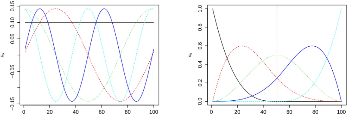
4.1 An example of Fourier (left) and B-spline (right) expansion withk=5 basis functions. . . 41

(12)

5.1 APX: Half-hourly price time series for the period 12/01/2014 - 18/01/2014. . . 50

5.2 APX: Daily price curves for the period 01/01/2014 - 31/12/2014. . . 51

5.3 (left) IPEX: Hourly demand cross correlation structure (right) PJM: Hourly prices cross correlation structure . . . 51

5.4 APX: Load period 9. log(Dt,j),fˆ1(Tt,j),fˆ2(Yt,j),and ˆf3(Wt,j)( ˆf3(Wt,j)is only for ten weeks) components. . . 54

5.5 Electricity Demand: Hourly MAPE values for (top left) PJM (top right) NP (middle) UKPX (bottom left) IPEX (bottom right) OMIE (Po). lines are (solid) VAR (dashed) FFAR (dot-ted) NPFFAR. . . 65

5.6 Electricity Price: Hourly MAPE values for (top left) NP (top right) APX (bottom left) PJM (bottom right) IPEX. lines are (solid) VAR (dashed) FFAR (dotted) NPFFAR. . . 71

6.1 Supply (blue) and two demand (red) hypothetical curves . . . 74

6.2 IPEX: Supply (red) and Demand (blue) curves (left) and their zoomed version (right) . . . 77

6.3 Supply and demand curves original (black) and smoothed (dotted red) . . . 81

6.4 IPEX load period 9: market clearing price (black) and equilibrium price (red) for 485 day. . . 82

6.5 IPEX: supply and demand curves in original (red) and forcasted (black) . . . 85

6.6 IPEX: what-if simulations: (left) Predicted supply and demand curves (dashed) with modified supply curves (solid) (right) and zoom on a neighbourhood of the intersection . . . 87

6.7 IPEX: what-if simulations: (left) original supply and demand curves (dashed) with modified supply curves (solid) (right) and zoom on a neighbourhood of the intersection . . . 87

(13)

List of Tables

5.1 Electricity Demand: Prediction accuracy statistics: AutoRegressive (AR),

Nonparamet-ric AutoRegressive (NPAR), Functional AutoRegressive (FAR), NonparametNonparamet-ric Functional AutoRegressive (NPFAR), Vector AutoRegressive (VAR), Functional Functional

AutoRe-gressive (FFAR), Nonparametric Functional Functional AutoReAutoRe-gressive (NPFFAR). . . . 61

5.2 Electricity Demand: P-values for the DM test for equal prediction accuracy versus the

alternative hypothesis that model in the row is more accurate than model in the column

(squared loss function used) . . . 63

5.3 Electricity Demand: Hourly DS-MAPE . . . 64

5.4 Electricity Price: Prediction accuracy statistics: AutoRegressive (AR), Nonparametric

toRegressive (NPAR), Functional AutoRegressive (FAR), Nonparametric Functional Au-toRegressive (NPFAR), Vector AuAu-toRegressive (VAR), Functional Functional

AutoRegres-sive (FFAR), Nonparametric Functional Functional AutoRegresAutoRegres-sive (NPFFAR). . . 68

5.5 Electricity Price: P-values for the DM test for equal prediction accuracy versus the alterna-tive hypothesis that model in the row is more accurate than model in the column (squared

loss function used) . . . 69

5.6 Electricity Price: Hourly DS-MAPE . . . 70

6.1 IPEX: Supply and demand bids . . . 79

6.2 IPEX: Prediction accuracy statistics: Nonparametric Functional Functional AutoRegressive (NPFFAR), Functional Functional AutoRegressive (FFAR), AutoRegressive Integrated Moving Average (ARIMA) . . . 83 6.3 IPEX: P-values for the DM test for equal prediction accuracy versus the

alternative hypothesis that model in the row is more accurate than model in the column (squared loss function used) . . . 84

(14)

(15)

Chapter 1 Introduction

1.1 Overview

Before the liberalization, electricity sector was fully controlled by state-owned companies. In this monopolistic structure, the variation in the electricity prices was minimal and the main attention was paid to demand forecasting and long-term planning and investment in this sector. The electricity sector undergone through drastic reforms in the late 80’s when the state owned monopolistic structure was reorganized into liberalized and competitive power markets. The main idea behind restructuring was to promote competition among generators, retailers and consumers by encouraging private investments in production, supply and retail sectors. The first electricity reforms were introduced in Chile in 1982, and in the follow-ing years the phenomenon spread throughout the world particularly in Europe. The British electricity sector started its liberalization in 1990 followed by Norway in 1992 and so on. Currently, many EU countries, including Italy, have their own liberalized electricity mar-ket as well as Australia, America, Canada, New Zealand, Japan and many other developed countries. The number of liberalized electricity markets is steadily growing worldwide, but the trend is most visible in Europe.

The liberalization not only brought important benefits to consumers such as low prices, more choices, reliable and secure electric supply but it also introduced a new field of research. The accurate modeling and forecasting of different variables related to the markets e.g. prices,

(16)

demand, production etc. became more crucial due to market structure. In most countries, the electricity market consists of different markets including a day-ahead market where prices and demand are determined the day before the delivery by means of (semi-) hourly concur-rent auctions for the next day. For each auction, producers/buyers submit their offers bids willing to sell/buy a certain amount of electricity at a given price. These bids are aggregated by an independent system operator in order to construct the aggregated supply and demand curve which determines the market clearing price and quantity. Since electricity is a flow commodity in the sense that it cannot be stored in large amount, over or under-estimation of electric load can cause serious problem to electric utility providers, energy suppliers, system operators and other market participants. For example, in case of underestimation, agents rely on highly responsive but expensive generating plants since low cost generating plants need a long time to start-up and so are not useful for serving short-duration peaks. On the other hand overestimation of electricity demand leads to unnecessary production or excessive purchases of energy which can cause substantial financial losses. Adequate fore-casting, instead, leads to less expensive, reliable and secure power operation and planning and allows the cash flow analysis, least cost planning, integrated resource planning, finan-cial procurement, regulatory rule-making and demand side management etc (Bunn, 2004a). However forecasting electricity markets are not straight forward due to the specific features these markets exhibit. There exist a large variability in end-user demand throughout the year due to seasonal variation resulting in multiple periodicities, non-constant mean and variance, spikes or sudden jumps etc. in the price and load series. Calendar effects are evident as the daily load and prices profiles are different for different days of the week and the behavior deviates from the typical behavior on bank holidays, bridging holidays etc. Technical problems such as plant outages and grid line unreliability add more variability to the system. The load series usually contain few outliers however; the price series show high volatility and unexpected jumps, also called spikes. In fact, the volatility is by far stronger for electricity prices compared to any other financial commodity (Weron, 2007).

In the literature, different methods have been discussed to account for these specific features effects before modeling the demand/price series in order to achieve stationarity and

(17)

mini-1.1 Overview 3 mizing distorting effects on forecasting. These effects are either modeled in a deterministic or stochastic way. In the deterministic approach, piecewise constant functions or dummies are widely used to model the multiple periodicities and the specific calendar conditions such as bank holidays, bridging effect etc. (Escribano et al., 2011; Fanone et al., 2013; Fleten et al., 2011; Gianfreda and Grossi, 2012; Lisi and Nan, 2014; Lucia and Schwartz, 2002). In some cases, components are modeled using sum of sinusoidal functions of different fre-quencies, sometime, equipped also with linear trend for the long term dynamics (Bierbrauer et al., 2007; Erlwein et al., 2010; Nan et al., 2014). Other authors considered polynomials, splines, wavelet decomposition, moving averages and in some cases state space models with linear trend to model different components (De Livera et al., 2011; Dordonnat et al., 2010; Janczura and Weron, 2010; Schlueter, 2010). In the second case, components are viewed as stochastic processes. Some authors suggest modeling of long term dynamics by a ran-dom walk or Brownian motion with the assumption of unit root while other also treated the seasonal components as stochastic (Bosco et al., 2010, 2007; Koopman et al., 2007). The stochastic approach is widely used for the case of spikes/jumps and is modeled by diffu-sion models with Poisson jumps or by Markov-switching models (Borovkova and Permana, 2006; Hellström et al., 2012; Pirino and Renò, 2010; Weron et al., 2004a,b). Lastly, it is worth mentioning that in both cases, deterministic or stochastic, the authors who modeled the specific calendar effects e.g. bank holidays, bridging effects etc. considered dummies. Once these components are estimated, the residuals (stochastic) component is obtained by subtracting them from original (unadjusted) demand/price time series, whose dynamics is modeled using different models with increasing level of complexity

For the modeling of residual part, two approaches can be considered, univariate and mul-tivariate. Since an individual auction is held for each load period and the load pattern is quite different across the different days of the week, the first approach treats each load pe-riod separately, consequently, (48)24 (half-)hourly models, reflecting the incorporation of the daily total series. However, the load profile suggests the presence of correlation among different load periods within a day that can be used when modeling the series and thus leads to a multivariate approach. For both approaches, various techniques have been

(18)

pro-posed in the literature, see for example (Weron, 2014, and references therein). Different parametric models, such as regression models (e.g multiple regression), time series models (e.g. ARIMA and its extensions) and models based on exponential smoothing techniques (e.g. Holt-winters and its extensions) that account for multiple seasonalities are extensively used (Bianco et al., 2009; Charlton and Singleton, 2014; De Livera et al., 2011; Ediger and Akar, 2007; Hong et al., 2010; Taylor, 2012). Semi-parametric and state space models are also employed to forecast short-term electric load and prices (Dordonnat et al., 2008; Fan and Hyndman, 2012). On the other hand, nonparametric techniques are always attractive for researchers due to their flexibility to functional form specifications, non-linearity and detection of structures that are usually undetected by traditional parametric methods. These techniques under dependence are useful for forecasting in time series and are frequently used (Härdle and Vieu, 1992; Hart, 1991; Shang et al., 2010). Artificial neural network (ANN) are extensively used for load forecasting due to their nonlinear and nonparametric features (Hippert et al., 2001; Zhang et al., 1998). Prediction problems are also addressed with other computational intelligence based methods such as fuzzy logic, support vector ma-chines etc. (Mohandes, 2002; Pandian et al., 2006). Although mathematical structure and complexity of all the models differ, it is difficult to find a single model that outperforms all others in every situation. In general, each model has its own advantages and disadvantages when it comes to practice.

1.2 Main contributions of the thesis

The main goal of this thesis is to model and forecast variables related to electricity markets such as, prices, demand etc. To this end, different approaches are considered and applied to electricity market data. This work considers the deterministic approach for the compo-nent estimation, and analyzes several ways of modeling the residual compocompo-nent. Both for demand and prices, different classes of models are estimated and compared in terms of fore-casting ability with respect to the original (unadjusted) time series. In particular, different univariate as well as multivariate models, parametric and nonparametric, have been

(19)

consid-1.2 Main contributions of the thesis 5 ered for five electricity markets, namely, British electricity market (APX Power UK), Nord Pool electricity market (NP), Italian electricity market (IPEX), Pennsylvania-New Jersey-Maryland electricity market (PJM) and Portuguese electricity market (OMIE(Po)). These markets substantially differ in generation modes, market maturity, size and policies imple-mented, geographical location and land electricity demand and have been widely consid-ered in the literature. Our data set consists of 24 (or 48) observations for each day, cor-responding to the number of daily auctions. The class of univariate models includes para-metric autoregressive models (AR), nonparapara-metric and nonlinear regression models based on splines (NPAR) and scalar-response functional models, that in turns can be formulated parametrically (FAR) or non parametrically (NPFAR). The multivariate models are vector autoregressive models (VAR) and functional-response, parametric (FFAR) and nonparamet-ric (NPFFAR), models. Linear AR(p) models are well-known and widely used (Brockwell and Davis, 2006). They describe the daily dynamics of load/price taking into account a linear combination of the last p values. In the nonparametric nonlinear (NPAR) case, the relation between current load/price and its lagged values has not a specific parametric form allowing, potentially, any kind of nonlinearity. Vector autoregressive (VAR) models are well-known multivariate models able to account for linear relationships among different time series. In this approach each variable (in our case the demand/price at each load pe-riod) is a linear function of past lags of itself and of the other variables. On the other hand, functional models consider the demand/price daily profile as a single functional object. Gen-erally, statistical models combine information either across or within sample units to make inference about the population, functional data analysis (FDA) considers both. Although functional data analysis has been extensively used in other fields, limited literature is avail-able for time series prediction and the books (Ferraty and Vieu, 2006; Ramsay et al., 2009) are comprehensive references for parametric and nonparametric functional data analysis. Its main advantage with respect to vector autoregressions (VAR) is that VAR are multivariate finite dimensional models, while functional models, being infinite dimensional, bypass the problem of the number of variables and allow to use additional information (e.g. smooth-ness, derivatives) contained in the functional structure of the data. The use of the functional

(20)

approach is one of the main contributions of this thesis. In fact, although it is not completely new, the use of the functional approach in the energy markets is not still widespread. In the following, the contents of the thesis have been divided in two points, corresponding to two different kinds of problems that have been considered.

1)The first part addresses the issue of modeling and out-of-sample forecasting electricity demand and price time series. To this end, I referred to the additive component model sug-gested by Lisi and Nan (2014) that assumes some deterministic components and a stochastic residual component. The deterministic components include a long-term dynamics, annual and weekly periodicities and calendar effects. Different possibilities for the estimation of these components were considered and the final selection was made based on the minimum prediction error. The first three components were estimated using splines while the calendar effects were modeled using dummy variables. In case of demand, data for indicated margin was available for APX and hence included as an extra covariate to the model. The demand structure for OMIE(Po) changed dramatically in the start of 2012 and therefore a dummy variable accounting for this level shift has been included to the model. For the prices, fore-casted demand used as an extra covariate in the model. All these extra covariates were found highly significant. For the residual component, different univariate and multivariate mod-els have been considered with increasing level of complexity. Within both classes, linear parametric and nonlinear nonparametric models as well as functional based models have been estimated and compared in a one day-ahead out-of-sample forecast framework. Data from 2009 to 2014 were used for all five electricity markets included in our study. The first five years were used for models estimation while the year 2014 was left for one day ahead out-of-sample forecast. Thus, globally, we have 365*24(48) = 8760(17520) one-day-ahead predictions allowing for a thorough analysis of the forecasting results. To compare the forecasting performance, global mean absolute percentage error (MAPE), daily specific mean absolute percentage error (DS-MAPE) and mean square percentage error (MSPE) were computed for each model. To assess the significance of the differences among differ-ent summary statistics, Diebold and Mariano (DM) (Diebold and Mariano, 1995) test for equal predictive accuracy was used.

(21)

1.2 Main contributions of the thesis 7 The results suggest, as expected, the multivariate approach leads to better results than the univariate one. Within univariate models, the results clearly showed superior performance of scalar-response functional models compared to others. The significance of the results were evaluated and confirmed by DM test. In case of multivariate models, the functional models perform generally better with VAR being a competitive model in some cases. The results also lead to another important finding correspond to the performance of parametric and nonparametric approach that showed strong linkage with underlying process. For IPEX and OMIE (Po), the nonparametric and nonlinear approach performs better, suggesting pos-sible nonlinearities in the underlying process. For the other three markets, the parametric approach produces better results. Lastly, the obtained results were compared with other works in the literature. Although different works refer to different time periods, we com-pare the results with the authors who used the same prediction accuracy statistics. The comparison suggests that our forecasting errors are smaller compared with the state-of-art prediction techniques used in the literature.

2)In the second part of this thesis the issue of electricity price forecasting is revisited and a completely and, at my best knowledge, new approach is used. It is based on the idea of modeling the daily supply and demand curves, predicting them and finding the intersection of the predicted curves in order to find the predicted market clearing price and volume. For this task the functional approach is quite suitable because for each given day, the number of bids data, corresponding to the number of producers/buyers in the market, is very large. Thus, finite dimensional (both univariate and multivariate) forecasting techniques cannot be used due to the large number of variables. On the contrary, functional models consider a single day as a single functional object and the bids, points on this functional object. In this approach, the raw bids data for demand and supply corresponding to each (half-) hour is first aggregated in a specific order. The functional approach converts the resulted piece wise curves into smooth functions using B-spline approximation. To consider the weekly periodicity, data are divided into seven groups representing a single day of week. Thus, e.g., for the prediction of Monday, the historical data from all available previous Mondays were used. The application of this approach is limited to the Italian market because it requires a

(22)

lot of data that are not always simple to obtain. Note that these data are available only with a eight-day-lag and thus, in a real context, eight-days-ahead forecasting is required. For this issue, parametric functional model (FFAR) and the nonlinear nonparametric counter-part (NPFFAR) were considered. As benchmark, an ARIMA model was fitted to the scalar time series corresponding to the clearing prices obtained from the crossing points of sup-ply and demand curves. In this case we obtained one-day-ahead predictions and compared to the results obtained with our functional approach. We consider data for the period Jan-uary 2014 to April 2015. The whole year 2014 is used for model estimation while the last four months are used for out-of-sample forecasts. Mean absolute error (MAE), root mean square error (RMSE) and MAPE were used to summaries the results. The results showed superior forecasting performance of our functional approach. In general, the MAE were significantly lower ranging from 5% to 20% for different load periods. The MAPE values showed the difference between 1% to 4% in favor of functional models. The significance of the differences was also confirmed by DM test. Among different models, the nonparametric functional model produces better results compared to parametric models.

Apart from the improvement in forecasting accuracy, it is important to stress that forecast-ing the entire demand/supply curves can substantially improve the supplier/buyer biddforecast-ing strategy resulting in a significant financial gain. Despite their good forecasting abilities for electricity price/demand, an important drawback related to the classical time series models is the fact that they do not provide insight to the supply and demand mechanism conse-quently to the price/demand formation process. With the current approach, if the forecasted curves are available, a trader who requires a moderate quantity to sell/buy can rise/lower the price by submitting an extra non-standard offer for an extra small quantity. As forecasting the whole curves gives deep insight into the market, our analysis showed that this strategy can significantly improve bidding strategies and maximize traders profit.

(23)

Chapter 2 Electricity Sector, Liberalization Process

and Specific Features

2.1 Introduction

Electricity is a unique commodity that is essential for the development of any society or country. It helps to utilize human abilities and capabilities to produce goods and services efficiently, communicate more easily and to trade all around the world. Humans poverty, health, education, income etc. are strongly linked with the availability of this commodity. According to world health organization (WHO), around three billion people lack access to modern fuels for cooking and heating and use traditional stoves burning biomass (wood, animal dung and crop waste) and coal resulting four million premature deaths every year. The impact of electricity on human life is very strong and therefore, extensive studies have been made in different directions related to this sector.

Electricity is itself not the primary source of energy but the energy released by other sources and converted by mankind for the use of end-user. These resources are broadly divided into two categories: renewable and nonrenewable. Renewable resources such as hydro, solar, wind etc. are replenished naturally and over relatively short periods of time. On the other hand, nonrenewable energy resources e.g. coal, nuclear, oil, natural gas etc. are available in limited supplies and usually take long period to replenished. Both the categories are mainly

(24)

made up of the following energy resources:

• Chemical energy is obtained through chemical reactions or absorbed in the creation of chemical compounds such as oil, coal, natural gas, biomass etc.

• Nuclear energyis obtained through the radioactive decay of some unstable nuclide’s such as plutonium, uranium etc.

• Potential energyis obtained through the forces of gravity pulling something towards earth. The most common is the one that stored in the water.

• Kinetic energyis obtained through the motion of an object. The most common form is that obtained through windmill that converts the energy of moving air into electricity. • Solar energyis obtained through conversion of sunlight into electricity, either directly

using photovoltaic (PV), or indirectly using concentrated solar power (CSP).

The marginal cost of producing electricity is different for different resources. Electricity generated from nuclear, hydro and wind have low generation cost compare to generated by other fuels such as coal, gas, diesel, etc. As the demand increases, more expensive gener-ation units are used for genergener-ation that result increase in electricity prices. Before

liberal-Generation ✲ Transmission ✲ Distribution ✲ System Operations ✲ Retail

Figure 2.1 The electricity value chain

ization, electricity firms were vertically integrated in five major components also known as “electricity value chain” given in Figure 2.1. They comprised of generation, transmission, distribution, system operations and retail.

• Generation refers to the process of installing a power plant and converting primary energy resource to electricity.

(25)

2.1 Introduction 11 • Transmission refers to the transportation/transmission of the generated electricity. Power plants are often installed far from the population and therefore high voltage transmission lines are installed which stepped up (transformed) the voltage to travel fast and cover long distances.

• Distributionrefers to providing low voltage electricity to homes and industries. Sub-stations receive high voltage electricity and step down the voltage for the delivery and use of end-users.

• System operatorrefers to the process of monitoring the system continuously and bal-ancing supply and demand to avoid electric grid blackouts. As demand fluctuates throughout the day, system operator monitors and balance the system throughout the day so that production and demand match perfectly and continuously.

• Retailrefers to the process of delivery service for sale to retail customers. The retail companies directly sell electricity to end-users and responsible for providing billing, customer services etc. facilities.

The economy of a country is heavily dependent on availability and efficient management of electricity. Any mismanagement or shortages results significant crises for the economy and for this reason, until late eighties, electricity sector was fully controlled by state owned companies and was highly regulated. In this monopolistic structure, the variations in the electricity prices were minimal and the main attention was paid to demand forecasting and long-term planning and investment in this sector. Inspired from the successful liberalization of various sectors of the economy, electricity sector undergone through drastic reforms in late eighties that reorganized the state owned monopolistic structure into liberalized and competitive power markets. The main aim behind liberalization was to rely on competitive forces to encourage investment and efficiency that benefits all the participants of the market and consequently the economy.

(26)

2.2 Electricity Markets Liberalization

The liberalization process started first in Chile in 1982 by introducing reforms, the 1982 Electricity act, to electricity sector that dissolve the state owned monopolistic structure by commercialization and part privatization followed by large scale privatization in 1986. The main idea behind liberalization was to increase industry efficiency, price stability, height-ened competition, and enhanced security of supply. Soon after deregulation, many (macro-) economic indicators show considerable improvements that encouraged this phenomenon to spread throughout the world. In Europe, the British electricity sector was the first that started its liberalization in 1990 followed by Norway in 1992 and so on. Currently, many EU countries, including Italy, have their own liberalized electricity market as well as Aus-tralia, America, Canada, New Zealand, Japan and many other developed countries.

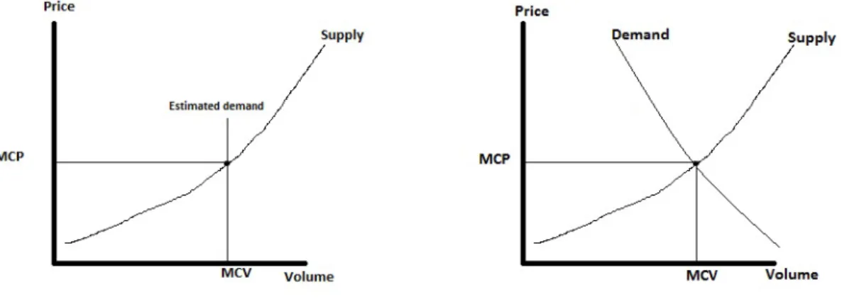
Electricity market reorganization unbundled the vertically integrated utilities that histori-cally managed generation, transportation and supply of electricity and introduce compe-tition mainly in generation and retail sector as all the competitors need non-discriminatory access to the other three components; transmission, distribution and system operations. Lib-eralization resulted mainly into two wholesale electricity markets; power pools and power exchange. The difference between these two is not trivial as they share many characteristics however they can be distinguish by two criteria: initiative and participation (Boisseleau, 2004). The power pools are the result of public initiative and the participation is mandatory i.e. no trading is allowed out side the pool while the power exchange is launched on private initiative and the participation is voluntary. Power pools are further divided into two types namely technical and economic pools. In technical pools, the power production cost and the network capacity is the main factor for dispatch. The power plants are ranked on merit order by their production cost and the electric utilities optimize their power generation with respect to cost minimization and optimal technical dispatch. Economic pools have been ini-tiated with the idea of competition among generators. This pool is one sided auction market where the participants are only generators and the participation is mandatory. In this mar-ket, the producers bid based on the prices for which they willing to run their power plants. These bids are aggregated to obtain supply curve by independent system operators. Finally,

(27)

2.2 Electricity Markets Liberalization 13 the market clearing price (MCP) and volume (MCV) are obtained through the intersection point of supply curve and estimated demand.

On the other hand, power exchange are two side auction markets where the market partic-ipants are generators, distributors, large consumers and traders. The main idea behind the establishment of power exchange was to facilitate the trade of electricity in a short term with the promotion of competition and liquidity. The market clearing prices (also called spot prices) and volumes are determined through two sided auctions in a day-ahead market where trading terminates typically the day before the delivery. Generally the auctions

con-Figure 2.2One and two side auction

ducted once per day where producers and buyers submit their offers bids willing to sell/buy a certain amount of electricity and its corresponding minimum price for each load period. These bids are aggregated by an independent system operator in order to construct the ag-gregated supply and demand curves which determine the market clearing price and quantity. The buyers who bid above or equal to market clearing price pay the price and the suppliers who bids below or equal are paid the same price. This pricing scheme is also called uniform pricing (non-discriminatory) in contrast to pay-as-bid (discriminatory) where a supplier is paid the amount for his transacted quantity based on his marginal cost.

Liberalized electricity markets are nowadays situated all around the world. These markets share many characteristics but also differ substantially in generation modes, market

(28)

ma-turity, size and policies implemented, geographical location and land electricity demand. From last two decades, extensive studies have been made on these markets in different di-rections. In the following, some of the markets that are considered in this thesis for empirical analysis are illustrated.

2.2.1 The British Electricity Market

The liberalization of UK electricity sector is due to structural changes and regulatory re-forms introduced in late 80’s in order to dissolve the state owned monopolistic structure and to introduce a competitive electricity wholesale market. Since transmission and distribution are natural monopolies, the main objective of the reforms was to privatised the generation and supply sector. Hence in 1990, the UK electricity market is reorganized into England and Wales electricity pool and the state owned monopoly is divided into three companies, namely, National Power, Powergen and Nuclear Electric. The pool was compulsory day-ahead one sided market where the trading was carried out on half-hourly basis. National Power and Powergen had 50% and 30% shares respectively due to which market power in generation was a significant problem as Nuclear Electric was providing the based load nu-clear power and essentially was a price taker. Market manipulation by these two companies resulted in a less competitive environment and hence the average price remain 24£/MWh in the years 1994-96 (Bunn, 2004b).

With the introduction of New Electricity Trading Arrangements (NETA) in 2001 (from 2005, NETA is called British Electricity Trading Transmission Arrangements, BETTA), the pool was replaced by fully liberalized bilateral contracting and voluntary spot trading market resulted in a balanced market share for electric utilities both in generation and retail sectors. These reforms resulted three independent power exchanges namely, UK Power ex-change (UKPX), UK Automated Power Exex-change (APX UK) and International Exex-change (IE, formerly named International Petroleum Exchange (IPE)). In 2004, APX and UKPX merged into APX Group and a year later, Scotland was included to the UK electricity mar-ket. Currently this market is fully competitive and one of the mature market in the world that exhibits strong linkage between market price and market fundamentals Karakatsani and

(29)

2.2 Electricity Markets Liberalization 15 Bunn (2008).

2.2.2 The Nordic Electricity Market

Soon after the liberalization of British electricity sector, the phenomenon spreads through-out the world, particularly in Europe. The Nordic electricity market was established in 1992 as a consequence of the reforms introduced in Norwegian energy act 1991. The deriving fac-tor for the reforms was the increasing dissatisfaction of electric secfac-tor performance in terms of economic efficiency in resource utilization. In the beginning, this market consisted of Norway only however in the preceding years Sweden (1996), Finland (1998) and Denmark (2000) were also included and was called Nord pool. Nord pool was the first international power exchange and currently over 380 companies from 20 countries actively trade on this market.

Nord pool electricity market is comprised of different markets. The day-ahead market (spot market) where power trading for physical delivery is carried out is called Elspot. The par-ticipation in this market is voluntary and the minimum contract size is 0.1 MWh. The prices are determined in a two-sided concurrent auction system (demand and supply) for each hour of the day. The resulted price is used as the reference price for settling financial power contracts and a benchmark for bilateral transactions. The adjustment market, Elbas is a short-term physical delivery market that allows players to modify the injection/withdrawal schedules that they have defined in Elspot. Eltermin and Eloption are financial markets that offer different kind of financial products.

The Nord pool electricity market is quite unique since the larger portion of electricity is gen-erated from hydro source. The electric production from hydro in Norway, Sweden and Ice-land are over 99, 85 and 76 percent respectively. The peculiar price dynamics are originated by this feature as prices are very sensitive to atmospheric conditions. Electric production varies from season to season depending on rainfall and snow conditions. The water short-age in 2002-2003 resulted in substantial price increase and put the electricity market under tremendous pressure. Consequently, all the Nordic power plants were used for production and significant increase in imports and decrease in demand was observed in that period.

(30)

2.2.3 The PJM Electricity Market

The PJM (Pennsylvania-New Jersey-Maryland) Interconnection is a regional transmission organization (RTO) that manages all the movement of wholesale electricity in all or parts of thirteen states and the District of Columbia in United States of America. It is an inde-pendent and neutral party that operates a competitive wholesale electricity market and also responsible to manage and ensure the reliability of high-voltage electricity grid that provide electricity to over 61 million people. The PJM Interconnection started the transition to an liberalized, independent and neutral organization in 1993 when the PJM Interconnection Association was formed to administer the power pool. In 1997, PJM became a fully in-dependent organization and opened its first bid-based energy market. The PJM announced as the nation’s first fully functioning independent system operator (ISO) in late 1997 and approved as a regional transmission organization (RTO) in 2001 to operate the transmission system in multi-state areas. From 2001, The PJM interconnection is growing continuously and a number of utilities transmission systems are integrated to PJM resulted in the world largest competitive market where continuous buying, selling and delivery of wholesale elec-tricity is carried out. The growing number of utilities integrated to PJM enhances its abilities to meet consumer demand for electricity with diversified resources availability.

The PJM consist of two generating capacity markets, two energy markets, an ancillary ser-vice market and a financial transmission entitlements market. The energy markets consist of two different market: (1) a day-ahead market where most of the quantity is traded through hourly auctions for the next operating day based on generation offers, demand bids, and bilateral transaction schedules submitted into the day-ahead market and (2) a real time (five minutes) market that is a real time balancing market where locational marginal prices are calculated at five minute intervals based on actual grid operating conditions.

2.2.4 The Italian Electricity Market

In Italy, the liberalization process of the electricity sector started in 1999 when the state-controlled entity, ENEL, was replaced with a market mechanisms more suited to the new

(31)

2.2 Electricity Markets Liberalization 17 framework for power trade. The main objective of liberalization was to regularize the mar-ket for electricity power production and trading under principles of neutrality, transparency, objectivity and competition among producers. The first regulated wholesale electricity mar-ket in Italy started to operate as a pool in April 2004. In 2005, the pool was replaced by an exchange namely Italian Power Exchange (IPEX) by liberalizing the demand side bidding. Since July 2007, when the market became fully liberalized, it has gone through different phases of market maturity. According to TERNA, the Italian transmission network opera-tor, the total electricity demand for the year 2014 was 309 TWh, a 3% decline from 2013, third consecutive annual decrease and is 10% lower than observed in 2007 when it reached to its maximum. Compared to 2013, net production decreased around 4%, and was 267.6 TWh resulted an increase in import by 3.7% (up to 43.7 TWh) that covers 14% of Italian demand. The price for base load showed a decline of 10 Euro/MWh compared to year 2013 and reached to 52.1 Euro/MWh, the lowest level in the last decade.

The Italian Spot Power Exchange is split in several markets namely the Day-ahead market (MGP), Adjustment/intra-daily market (MA) and the Ancillary services market (MSD). The Gestore dei Mercati Energetici S.p.A (GME) is responsible for scheduling injections and withdrawals of electricity for the next day in 24 concurrent auctions one each for a hour in a day. The adjustment market (MA) allows the utilities to modify their injection/withdrawal schedules defined in MGP. TERNA use the MSD to retrieve the resources required for con-trolling the power system, i.e the creation of an energy reserve and real-time balancing. The Italian electricity market is divided into different zones and the prices across the zones can differ due to transmission limits and supplier’s behaviour. With the introduction of Italian derivatives energy exchange, producers and consumers are allowed to hedge positions, to have bilateral contracts for the prices far in the future and to physically trade energy.

2.2.5 The OMEI(Po) Electricity Market

Spain was the first Iberian country that liberalized its electricity sector. In 1997, Operadore del Mercasdo Espanol de Electricidad (OMEL) was created to manage and run wholesale electricity market. In November 2001, the formation of an Iberian electricity market

(32)

(MI-BEL) is initiated by Portuguese and Spanish governments however the start of the joint organized market took longer due to many political and technical reasons. In July 2006, MIBEL start its operations in both, Portugal and Spain. Like any other market, the Iberian electricity market has a day-ahead and intra-daily markets. OMEL has changed its name to Operador Del Mercadeo Iberico De Energia (OMIE, operator of the Iberian Market) and is in charge of managing the MIBEL day-ahead market where electricity is traded on hourly basis for the twenty-four hours of the following day. In the intra-day markets, buyers and sellers are allowed to readjust their commitment made in day-ahead market for purchasing and selling up to four hours ahead of real time. In 2014, OMIE covers 80% trading of electricity amounting for 11 billion Euros carried out in Spain and Portugal. With over 800 participants, this market is one of Europe’s more liquid ones and the prices are generally below the average compare to Europe’s major markets.

2.2.6 Other Electricity Markets

Nowadays liberalized electricity markets are situated all around the world. In Europe, in-cluding above mentioned countries, Austria, Belgium, Czech Republic, Estonia, France, Finland, Germany, Hungary, Latvia, Lithuania, Luxemburg, the Netherlands, Poland, Ro-mania, Slovakia and Slovenia liberalized their electricity sector. Many developed countries e.g. Australia, Japan, Turkey, America, Canada etc. have their own liberalized electric-ity market. The main motive behind liberalizing and restructuring electricelectric-ity market in all countries is to ensure security of supply and efficient production by introducing competition in different sectors.

2.3 Electricity Time Series Features

Liberalization not only brought important benefits to consumers such as low prices, more choices, reliable and secure electric supply but it also introduced a new field of research. The accurate modeling and forecasting of different variables related to these markets e.g. prices, demand, production etc. became more crucial due to market structure. Electric utilities,

(33)

2.3 Electricity Time Series Features 19 generators, system operators and other participants are highly interested in forecasting these variables at different horizons, that are referred in the literature as short-, medium- and long-term. Daily and weekly predictions are very common and are used for real time operations, control of power system and generator maintenance whereas monthly and yearly maximum and minimum loads are important for planning purposes and risk management studies. In the literature, short-term prediction received higher attention because in many electricity markets daily demand and prices are determined the day before the delivery by mean of (semi-)hourly auctions for the following day. Therefore efficient modeling and forecasting for these variables is an important issue in competitive electricity markets. However this task is challenging due to the specific features these markets exhibit that are substantially different from other financial commodities markets and hence require dedicated modeling techniques. A physical constraint to electricity is that it cannot be economically stored and must be delivered to end-user at the time when it is produced. Due to this characteristic, minor fluctuations in electricity demand can cause serious problems for electric utilities, generators, distributors and other market participants. The main peculiarity referring to price volatility is also attributed to this characteristic. On the other hand, the end user treats electricity as a facility resulting the demand to vary throughout the day, week and year. These and other attributes generate different features found in both, demand and prices time series that are commonly shared across the electricity markets. In the following, some of the main features found in demand and prices series are described.

2.3.1 Seasonality and Calendar Effects

Perhaps the most common and prominent features that the electricity demand exhibit are seasonality and calendar effects. In most markets, electricity demand shows three regular cycles: daily, weekly and annual. An example of the three periodicities is given in Fig-ure 2.3. Annual cycle can be clearly seen from the graph as the variation in the demand level throughout the year has similar pattern in both years. Daily cycle is evident from the similarity of the demand from one day to the next whereas an weekly cycle can be seen by comparing the demand level on same days of different weeks. Electric consumption is

(34)

Year Demand MWh 30000 50000 2009 2010 2011 26000 0 50 100 150 200 250 300 350 30000 34000 38000 Days Demand MWh

Figure 2.3APX: (left) Annual seasonality for the period 01/01/2009 - 31/12/2010. (right) NP: Daily and weekly periodicity for demand data in the period 24/04/2010 - 07/05/2010.

closely related to human behaviour, daily life and economical activities. The daily cycle is responsible for the highest part of variability in the data (see Figure 2.4). The consumption varies throughout the day and night following the working habit of population that can be seen in Figures 2.5. The demand is considerably lower at night and starts increasing in the morning when people start their daily life. Depending on the market, the daily cycle can have one or more peaks during the day corresponding to the living habits of the population and atmospheric conditions of the country. Due to this variation, many researchers argued

(35)

2.3 Electricity Time Series Features 21 and considered the daily load pattern as (48)24 (half-)hourly different time series for mod-eling purposes. The weekly cycle encompasses for relatively lower variation in the data. As

Hour Demand MWh 0 5 10 15 20 25 75000 85000 95000 Hour Demand MWh 0 5 10 15 20 25 32000 36000 40000

Figure 2.5Average daily curves for the period 01/01/2014 to 31/12/2014 for (right) NP (left) PJM

can be seen in Figure 2.6, load profiles are relatively different on different days of the week. Saturday and Sunday load profiles are considerably lower than those of other weekdays. In general, demand is lower during national holidays, bridge holidays (a day between two

0 5 10 15 20 25 20000 30000 40000 50000 Hour Demand MWh

Figure 2.6 IPEX: Daily demand curves for the period 1/4/2011 - 30/4/2011. Solid lines: weekdays; dashed lines: Saturdays; dotted lines: Sundays. Solid line at the bottom: bank holiday (25th April).

(36)

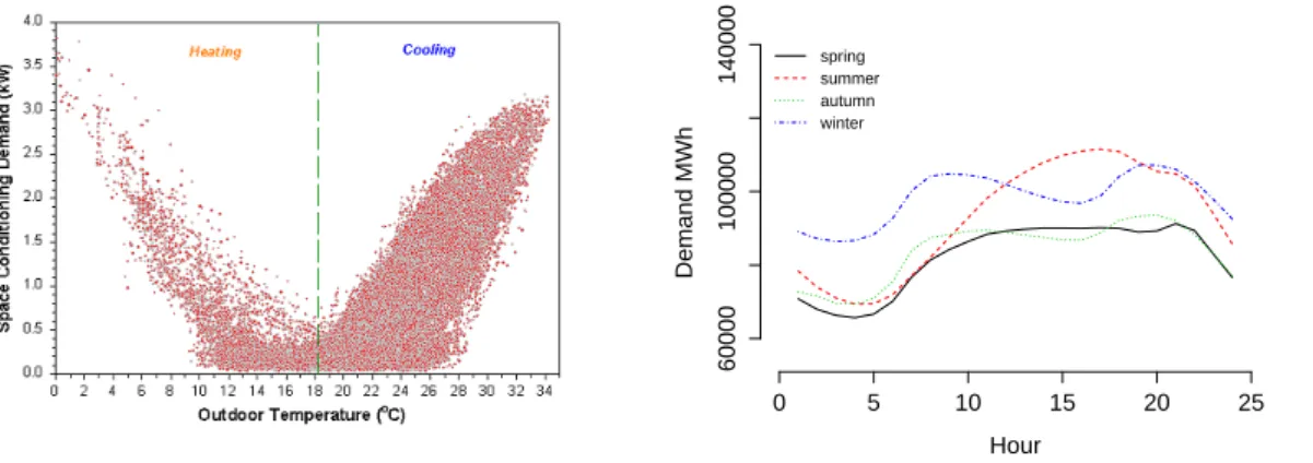
not-working day) and any other not-working day. A steep decline on late Friday and a steep increasing on Monday morning are commonly observed in load data. This feature is also called “weekend effect” and is also present during other not-working days. This characteris-tic often affect electricity prices as the prices on Saturdays, Sundays and other not-working days are relatively unstable compare to other days. Annual periodicity is often referred to the seasonal fluctuations caused by variation in temperature and length of day. As can be seen from Figure 2.7, the electricity consumption is higher during summer and winter due to the growing use of air conditioning and heating, respectively, and is lower in autumn and spring. In fact, atmospheric conditions such as wind velocity, cloud cover, humidity,

pre-Hour Demand MWh 0 5 10 15 20 25 60000 100000 140000 spring summer autumn winter

Figure 2.7 (left): Temperature Vs electricity demand (source: Parker (2003)).(right) IPEX: Average daily electricity demand in each season for 2014.

cipitation, rainfall and snowfall not only originate the yearly cycle but also explain the short term variation in electricity demand. In general, electricity demand and atmospheric tem-perature hold strong nonlinear relationship as can be seen from the Figure 2.7. In addition, the prolong use of artificial lights also assert to the demand increase in winter.

2.3.2 Volatility, Outliers and Jumps

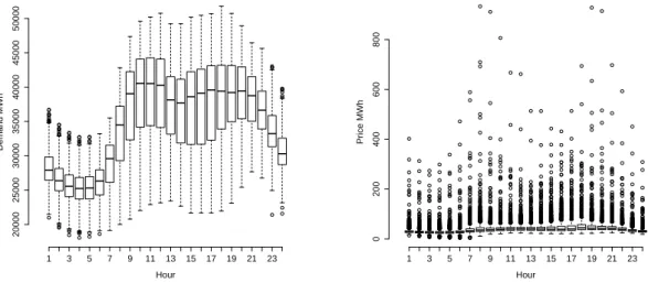
Electricity demand often contain few outliers however; the price series show high volatility and unexpected jumps (also called spikes) due to meteorological, economical, technical and other influential factors. Figure 2.8 shows an example of outliers and volatility in demand

(37)

2.3 Electricity Time Series Features 23 and prices data respectively. Price volatility is known as one of the most pronounced fea-tures and a direct consequence of electricity market liberalization. Electricity spot prices are highly volatile and the price can vary extremely within a short period of time. In fact, the

1 3 5 7 9 11 13 15 17 19 21 23 20000 25000 30000 35000 40000 45000 50000 Hour Demand MWh 1 3 5 7 9 11 13 15 17 19 21 23 0 200 400 600 800 Hour Pr ice MWh

Figure 2.8 (left) IPEX: Box plots for hourly demand for the period 01/01/2009 - 31/12/2014. (right) PJM: Box plots for hourly prices for the period 01/01/2009 - 31/12/2014

volatility is by far stronger for electricity prices compared to any other financial commodity. Price spikes or jumps that are known as short lived, abrupt and generally unanticipated ex-treme price changes are commonly observe in electricity price series. In Figure 2.9 (left), an example of this feature is given when the spot prices increases substantially to many folds of its normal value and then drops back to the previous level soon after. Generally, these price spikes are short lived and much more extreme in magnitude. To understand well the reasons of these spikes, one should remember that electricity markets have distribution and trans-mission constraints that make them different from other commodity markets. Electricity cannot be economically stored and it has capacity and transmission constraint as well as the system must be balanced in real times. Any temporary imbalance in supply and demand due to any influential factor or technical reasons can cause price spikes. An important market structure element that plays vital role in market price determination is the diversity of gen-eration plants and their corresponding marginal costs per unit of production. A schematic supply stack corresponding to different sources of energy with two potential demand curves

(38)

Years Pr ice MWh 0 200 400 600 800 2013 2014 2015

Figure 2.9 (left) PJM: Hourly electricity spot prices for the period 01/01/2013 - 31/12/2014. (right) A schematic supply stack with superimposed two potential demand curves (source Weron et al. (2004b))

superimposed is given in Figure 2.9 (right). As can be seen from the graph when the de-mand is low, electricity is produced and supplied from low marginal cost sources. As soon as the demand increases, the marginal production cost increases since the more expensive fuels plants start operations. Even a small increase in electricity demand can force prices to increase substantially. Once the cause of spike goes away, the prices fall back to their average level. Price spikes are non constant and are highly variable with respect to time scale. In general, they occur during peak load hours when the electric consumption is high.

2.3.3 Non-normality and Non-stationarity

In most electricity markets, the distributional properties of the spot electricity price series appear non-normal and highly positively skewed. For instance, Figure 2.10 shows these features for the PJM market for the period 01/01/2009 to 31/12/2010. The histogram shows positive skewness suggesting the greater likelihood of large price increases than price falls. Some authors suggest that the leptokurtic or heavy tailed feature indicates of inverse lever-age effect. This means that positive jumps in prices amplify the conditional variance of the underlying process more than negative ones. On the other hand, extensive literature argued about the possible non stationarity of the demand series. In general, it has been widely observed and described that electricity demand series are non-stationary. Apart from other

(39)

2.3 Electricity Time Series Features 25 price probability density 0 50 100 150 200 0.000 0.010 0.020 0.030 −4 −2 0 2 4 1 2 3 4 5 6

Quantiles of normal distribution

Quantiles of logar

ithmic pr

ices

Figure 2.10PJM: hourly electricity spot prices for the period 01/01/2009 to 31/12/2010. (left) Normalized histogram with superimposed nonparametric density in red (right) quantile-quantile plot

features it exhibit, electricity demand shows an overall trend due to the country economic situation, atmospheric changes, technological advancement and other related factors. For example, demand data for APX and PJM markets are plotted in Figure 2.11 that shows an overall trend. Generally, the trend can be increasing/decreasing and linear or nonlinear. In the case of APX, one can see that data exhibit a linear trend where for PJM, a nonlinear trend is more appropriate. In some cases, structural breaks or level shifts (see for example Fig-ure 2.11) are also observed in demand series that are generally resulted from the expansion of the market or by the introduction of new regulatory laws.

Year Demand MWh 25000 30000 35000 40000 45000 50000 2006 2007 2008 2009 2010 2011 2012 2013 2014 2015 Year Demand MWh 20000 40000 60000 80000 100000 2001 2003 2005 2007 2009 2011 2013 2015

Figure 2.11 Daily electricity demand for (right) APX, for the period 01/01/2006 - 31/12/2014 and (left) PJM, for the period 01/01/2001 - 31/12/2014 with superimposed linear (red) and a nonlinear (green) trend.

(40)

2.3.4 Mean Reversion and Other Features

In general, electricity prices are regarded to be mean-reverting. Mean reversion is a process refers to a stochastic process that displays a tendency to remain near or to revert to its histor-ical mean value. In other words, this process suggests that prices or returns eventually move back towards the overall mean of underlying commodity. As explained in section 2.3.2, in electricity market any temporary imbalance in supply and demand can cause a price spike. However, once the cause of spike goes away, the prices fall back to their average level sug-gesting strong mean reversion characteristics in price series (see for example Figure 2.12). On the other hand, in some markets (e.g. the French and German/Austrian day-ahead

mar-0 200 400 600 800 1000 0 50 100 150 200 Half hour Pr ice

Figure 2.12(left) APX: Half-hourly electricity prices (right) Hourly electricity prices for European Energy Exchange (source Erni (2012))

ket) electricity prices can turn negative when a high inflexible generation hit a low demand. Inflexible power resources (e.g. Nuclear) cannot be shut down and restarted in a fast and cost efficient manner. In case of low demand, prices fall signalling generators to reduce production in order to avoid overloading of the grid. In this case, often generators accept negative prices as it is less expensive to keep power plant online than to shut down.