San Jose State University
SJSU ScholarWorks
Master's Projects Master's Theses and Graduate Research
Spring 5-10-2019
Assessing Code Obfuscation of Metamorphic
JavaScript
Kaushik Murli
San Jose State University
Follow this and additional works at:https://scholarworks.sjsu.edu/etd_projects
Part of theArtificial Intelligence and Robotics Commons, and theInformation Security Commons
This Master's Project is brought to you for free and open access by the Master's Theses and Graduate Research at SJSU ScholarWorks. It has been accepted for inclusion in Master's Projects by an authorized administrator of SJSU ScholarWorks. For more information, please contact
Recommended Citation
Murli, Kaushik, "Assessing Code Obfuscation of Metamorphic JavaScript" (2019).Master's Projects. 667. DOI: https://doi.org/10.31979/etd.c2cn-mpyd
Assessing Code Obfuscation of Metamorphic JavaScript
A Project Presented to
The Faculty of the Department of Computer Science San José State University
In Partial Fulfillment
of the Requirements for the Degree Master of Science
by Kaushik Murli
© 2019 Kaushik Murli
The Designated Project Committee Approves the Project Titled Assessing Code Obfuscation of Metamorphic JavaScript
by Kaushik Murli
APPROVED FOR THE DEPARTMENT OF COMPUTER SCIENCE SAN JOSÉ STATE UNIVERSITY
May 2019
Dr. Thomas Austin Department of Computer Science
Prof. Fabio Di Troia Department of Computer Science
ABSTRACT
Assessing Code Obfuscation of Metamorphic JavaScript by Kaushik Murli
Metamorphic malware is one of the biggest and most ubiquitous threats in the digital world. It can be used to morph the structure of the target code without changing the underlying functionality of the code, thus making it very difficult to detect using signature-based detection and heuristic analysis.
The focus of this project is to analyze Metamorphic JavaScript malware and techniques that can be used to mutate the code in JavaScript. To assess the capabilities of the metamorphic engine, we performed experiments to visualize the degree of code morphing. Further, this project discusses potential methods that have been used to detect metamorphic malware and their potential limitations. Based on the experiments performed, SVM has shown promise when it comes to detecting and classifying metamorphic code with a high accuracy. An accuracy of 86% is observed when classifying benign, malware and metamorphic files.
Keywords- Metamorphic malware, Signature detection, Heuristic
ACKNOWLEDGMENTS
I would like to express my gratitude to my advisor Dr. Thomas Austin for giving me the opportunity to work on this project and for his support and continuous guidance. I am also very thankful to Prof. Fabio Di Troia for his invaluable feedback and for always nudging me in the right direction to improve the project and to Dr. Philip Heller for his valuable time and monitoring the progress of the project. Finally, I would like to thank my friends and family for their encouragement and their assistance, without whom I would have never completed this project.
TABLE OF CONTENTS CHAPTER 1 Introduction . . . 1 2 Background . . . 3 2.1 Types of malware . . . 3 2.1.1 Encrypted Malware . . . 3 2.1.2 Polymorphic malware . . . 3 2.1.3 Metamorphic Malware . . . 4 2.2 Obfuscation Techniques . . . 4 2.2.1 Instruction Substitution . . . 5 2.2.2 Instruction Renaming . . . 5 2.2.3 Instruction Reordering . . . 5
2.2.4 Dead Code Insertion . . . 5
2.3 Detection Techniques . . . 6
2.3.1 Signature-Based Detection . . . 6
2.3.2 Anomaly Based Detection . . . 6
2.3.3 Heuristic Analysis . . . 7 3 Metamorphic Techniques. . . 10 3.1 Implementation . . . 10 3.2 Instruction Renaming . . . 11 3.3 Instruction Reordering . . . 13 3.4 Instruction Substitution . . . 15
3.5 String Splitting . . . 16
3.6 Dead Code Insertion . . . 18
4 Assessing modification extent using Similarity Graphs . . . 19
4.1 Rhino . . . 19
4.2 Similarity Graphs . . . 20
5 Support vector machines. . . 25
5.1 Implementation . . . 27
6 Experiments and Results . . . 31
6.1 Similarity Graphs: . . . 32
6.1.1 Sliding windows . . . 32
6.1.2 Experimenting with each of the techniques . . . 34
6.2 SVM: . . . 40
6.2.1 Experiment1: Opcode Length . . . 41
6.2.2 Experiment 2: Parameter tuning for SVC . . . 43
6.2.3 Experiment 3: Adding new classes to the classification. . . 44
7 Conclusion and Future Work . . . 47
LIST OF TABLES
1 30 most occurring opcodes and their symbols . . . 28
2 System configuration’s . . . 31
3 Breakdown of benign files list . . . 32
4 Number of Files to the SVM . . . 40
5 Training and Test data split . . . 40
6 Classes and their representation . . . 44
7 Number of Files to the SVM . . . 45
LIST OF FIGURES
1 Polymorphic Malware Infection [1] . . . 4
2 Overview of the design flow . . . 10
3 Metamorphic Engine at work. . . 12
4 Results of Instruction Renaming . . . 13
5 An snippet of the hashmap . . . 14
6 A more complex AST . . . 15
7 Result of Instruction Reordering. . . 16
8 Result of Instruction Substitution. . . 17
9 Result of String Splitting. . . 18
10 Converting file to appropriate format . . . 21
11 A sample file after converting to bytecode. . . 22
12 Assessing extent of metamorphism.[2] . . . 23
13 A HyperPlane [3] . . . 25
14 Set of Possible Hyperplanes[3] . . . 26
15 Sliding window of 2. . . 33
16 Sliding window of 3. . . 34
17 Sliding window of 5. . . 34
18 A file matched against itself. . . 35
19 Instruction Renaming. . . 36
20 Instruction Reordering. . . 36
22 Dead Code Insertion. . . 38
24 ROC curve for Experiment 1. . . 42
25 Ideal parameters that give best accuracy. . . 44
CHAPTER 1 Introduction
Malware - short for malicious software is designed to penetrate and harm computers without the knowledge of the user. Malware can take up any form of executable code or script. The code/script is described as spyware, virus, worm, or keylogger. Early versions of malware were very primitive but abundant. Malware can infiltrate computers by a number of user actions such as by downloading free software, websites that can be infected via malicious code [4] and opening an email that contains a harmful attachment. A study revealed that cybercrime cost be-tween $400 and $608 million in the year 2017, $100 million more than the year 2014 [5].
A signature of a malware consists of a sequence of bytes. Large files consisting of these signatures could be used to detect any malware. This technique is called signature detection and is used to date in most commercial antivirus software. Signature detection is particularly useful at detecting known malware and also can be used to detect a large number of malware families.
To work around the ability of signature detection, metamorphic malware is used. To disguise malicious code, this malware is capable of rewriting its structure and thereby its signature with each iteration without changing its underlying functionality. JavaScript is useful to perform this obfuscation. Metamorphic malware can easily evade signature detection since the malware can create variants of the code that have a different signature compared to the original file.
This paper is organized in the following manner. Chapter 2 provides a background about the different types of malware, techniques to generate metamorphic malware
of the techniques that are used to obfuscate code by metamorphic engines along with their benefits. Chapter 4 covers the various experiments we will be running using opcode similarity. Chapter 5 covers detection techniques that can be explored such as Hidden Markov Models. Chapter 6 contains the conclusions and future scope of the project. The articles selected for this project include thesis projects, published papers and articles by companies in the field of malware.
CHAPTER 2 Background 2.1 Types of malware
Malware can be categorized into different classes based on the method of infection. Examples of these classes are worms, trojans, virus, spyware, rootkit, or keyloggers. Commercial anti-virus software uses signature-based detection technique to detect malware. A major drawback of signature-based detection is that it is not able to identify new malware or strains of malware that are not present in the signature file. Seeing an inherent weakness in this technique, malware writers mutate their code to change the malware’s signature. Several types of malware obfuscate their code to making it harder to analyze and be detected. Some of the types are described below.
2.1.1 Encrypted Malware
Encrypted malware was designed as a technique to evade signature detection. It contains the main virus body in encrypted format and a decryption routine. When the infected application is executed, the main virus body is decrypted using the decryption routine and it carries out its intended function, thus evading signature detection. Cascade which emerged in 1987 was the first of this type of malware [6]. The drawback of this method is that the decryption routine always remains the same and this can be used to detect the encrypted malware.
2.1.2 Polymorphic malware
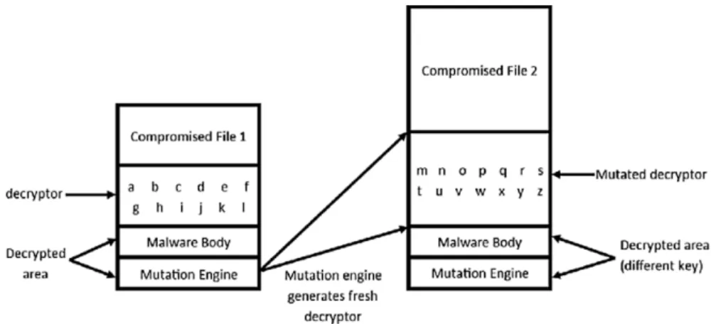
To overcome the weakness of encrypted malware, polymorphic malware was designed. When the infected program is executed, the malware is decrypted and carries out its intended function. In each execution, a new version of the malware is encrypted and stored for the next execution. The decryption routine is morphed after each iteration changing the signature constantly. Thus, the malware cannot be traced back by looking for bits in the decryption routine [7]. This malware was a
cutting-edge antivirus software. This is done by running the executable in an isolated environment, dissembling it and extracting the original virus body.
Fig. 2 shows a polymorphic malware in each cycle.
Figure 1: Polymorphic Malware Infection [1]
2.1.3 Metamorphic Malware
Metamorphic malware is a more advanced form of polymorphic malware that has proved to be harder to detect. In metamorphic malware, the virus body and the decryption routine are morphed after every iteration but retain the functionality [8] of the original code. The end result is that for two copies of the same malware, the obfuscated code bears no resemblance to the initial code. The first metamorphic malware ‘Win95/Regswap’ was released in 1989 [9]. The obfuscation techniques used can be divided into two parts namely data flow obfuscation and control flow obfuscation.
2.2 Obfuscation Techniques
Obfuscation techniques are used in metamorphic malware to evade detection tools. Some of the techniques are mentioned below and used with great success Troia et al.[10] and Musale et al.[7].
2.2.1 Instruction Substitution
This method replaces an instruction or a group of instruction with equivalent instructions whilst maintaining the same functionality [7]. Examples of this tech-nique are replacing a ‘mov’ operation with a push/pop sequence or replacing a ‘xor’ instruction with a sub-instruction.
2.2.2 Instruction Renaming
This technique looks for keywords such as ‘var’,‘def’ or ‘function’ and replaces the name with a randomly generated string [7].
2.2.3 Instruction Reordering
Independent instructions are switched using this technique. Only instructions that are in the same program scope are reordered. This gives a large number of morphed versions of the initial code [11]. Based on the number of independent instructions, say n, n! morphed versions can be generated.
Troia et al.[10] and Musale et al.[7] employ similar styles of instruction reordering but with subtle differences in the format. The style followed by [10] is an identifier followed by a "|" and a number to indicate dependency to an instruction. However, both representations achieve similar results.
2.2.4 Dead Code Insertion
In this method, instructions which do not affect execution are inserted to create morphed copies of the malware [7]. These instructions are called "do-nothing" [7] instructions and were used to create Win95/ZPerm [12]. Examples of such instructions are NOP (No operation) and INC (Increment) followed by DEC (Decrement) to give the original value. These instructions can be inserted anywhere in the global scope between two instructions. This technique is particularly useful in altering the structure of the code thereby changing the signature significantly. The drawback of this method is that it is slow since the whole file must be scanned to find the possible positions to
insert the dead code.
2.3 Detection Techniques
2.3.1 Signature-Based Detection
Since the first days of security monitoring, signature-based detection has been used. The main reason for its popularity is its low false positive rates, its ability to detect a large number of families of malware, and its low complexity. A known virus database of signatures is compared against the malware to identify it. The signature is the fingerprint of a file. In signature-based detection, a file is scanned and its signature is compared against the collection of signatures present in the database to determine for a match. However, this method has two main drawbacks. First, it cannot be used to detect malware that are previously unknown. Second, the contents of the database keep increasing which makes it harder to maintain. As the size increases so does the storage and the time required to match the signature. This method can be easily beaten using obfuscation techniques which constantly changes the signature.
2.3.2 Anomaly Based Detection
Anomaly-based detection monitors system activity to determine if the behavior of the system is normal or anomalous [11]. Unlike signature-based detection which looks for the signature of the malware, this classification is based on rules/heuristics and tries to determine if the system deviates from normal behavior. The main requirement for this detection technique is to understand what normal behavior is. Idika et al.[11] describes two main phases which is the training and testing phase occur. In the training phase, the detector attempts to learn what the normal behavior is and in the testing phase, the detector compares the current system behavior to the behavior in the training phase. A particularly useful feature of this technique is the ability to detect unknown malware since it categorizes anything that deviates from the normal behavior to be an attack. This also brings about a big drawback which is the fact
that it has a very high false positive rate and high complexity [11]. Another major drawback is that it is not easy to define normal behavior in more complex networks.
2.3.3 Heuristic Analysis
Heuristic Analysis is used to check for features that are considered suspicious in files. It is particularly useful for detecting variants of an existing virus family [13]. A drawback of this technique is the number of false positives. When a benign program is marked as a malware, it destroys the user’s trust over time. Users could assume that real malware is a false alarm and make the system more vulnerable.
It relies primarily on data sets and machine learning techniques to detect malware. Some of the machine learning techniques used are Data Mining, Neural Networks, Hidden Markov Models, and Support Vector Machines.
Malware can be considered as a sequence of events and thus Hidden Markov Models (HMM) and Support Vector Machines (SVM) are apt tools that can be used to detect it as it uses pattern recognition. HMM are useful in bio-informatics, reinforcement learning and pattern recognition such as speech, gesture, and handwriting. A Hidden Markov Model (HMM) is a state machine, which captures probabilistic dependencies between observed states and unobserved states, commonly called as hidden states. HMMs can be used to find the best combination of hidden states, give an observation sequence. For a given number of hidden states, the model looks at the data and constructs a hidden state transition matrix A and an emission probability matrix B. The features of the input data are represented as states of the trained HMM and the probabilities represent the statistical properties of the features. A Support Vector Machine (SVM) can be trained on a set of data which is also in the form of an observation sequence. Using SVM and its hyperplane [3], an optimal hyperplane can be calculated and used to classify data into separate classes.
sequences. Sequences from the original code and from the morphed code are extracted and then compared against each other for similarity. A score can be used to represent the similarity of the sequence using the trained HMM. The higher the similarity score is, the more similar the sequence is to the training data. Morphed variants of malware are generated using Next Generation Virus Construction Kit (NGVCK). Using a threshold value, the detection rate of this method was between 97.1 to 97.5% with a false positive rate of 3%. A limitation of this method is that it was unable to detect specifically designed metamorphic malware generated from engines such as MetaPHOR and MWOR[4].
A dueling HMM strategy is followed to better understand the hidden states in depth [12]. HMM are examined for four different compilers, hand-written assembly code, and three virus construction kits. Based on their experiments it is shown that the dueling HMM strategy can better detect malware than the method employed by Wong et al. [13][14].
Other methods have also been employed with some effect in detecting metamorphic malware. Bruschi et al. [15] employs a method that is used to undo the transformations done by the metamorphic engine. The program is normalized to its canonical form which is simpler in terms of structure while retaining the original semantics i.e removes all the techniques used during the metamorphosis. The drawback is that dynamic behavior of the malware cannot be characterized. Mohammed et al. [16] employs another method that reduces the morphed code to the respective zero form. This method shows promise but is not used on actual viruses. Although not used very frequently in malware detection, experiments have been performed for malware detection with SVM’s in the past. In 2013, Santos et al. [17] stated that SVM outperforms other classifiers using term frequency for different classifiers and obtained an accuracy of 92.92% for a one opcode sequence and an accuracy of 95.90% for a two
opcode sequence. In 2015, Ranveer et al. [18] proposed a method which achieved a True Positive Rate (TPR) of 1 with bigger test data set’s. This model is incredibly accurate in terms of classification as this proposed system considers both static and dynamic features.
CHAPTER 3 Metamorphic Techniques 3.1 Implementation
The design architecture is as follows, JavaScript code is converted to an Abstract Syntax Tree (AST) to perform the obfuscation techniques and then back to JavaScript to give the morphed code. To do this, a JavaScript parser ‘Esprima’ and a package
Figure 2: Overview of the design flow
known as Escodegen is used. Esprima is a high performance, standard compliant JavaScript Parser. This is used in Node.js to produce a beautiful syntax tree to work with.
An abstract syntax tree (AST), or just syntax tree, is a tree representation of the abstract syntactic structure of source code written in a programming language. Each node of the tree denotes a construct occurring in the source code. A simple expression var a = 6 * 7 produces the tree shown below. The variable a is present under the ‘VariableDeclarator’ with an identifier name as ‘a’. 6 * 7 corresponds to a binary expression with the left and right of the tree being the value. Escodegen gives back JavaScript code which is then written into the output div tag. This is used in Node.js by using the following command.
var escodegen = r e q u i r e ( escodegen ) ; var newCode = escodegen . generate (AST) ;
This approach was selected due to its simplicity and allows to make changes to the AST progressively.
The aim was to see which features can be converted back to JS from the tree. All the techniques could be converted back to JS aside from String splitting. One of the drawbacks was that we cannot convert code back into JS inside loops using Escodegen. Alternative methods could be employed but the output would not be visually pleasing. A figure below shows the metamorphic engine.
3.2 Instruction Renaming
As seen in the experiments, variable and function renaming is one of the more effective obfuscation techniques. Using this method, we scan for keywords such as var and function in the whole script file and replaces the name of a variable/ function with a randomized two letter string.This consequently changes the signature of the program repeatedly. All the occurrences of a string are changed within the same scope. An example of our application in action is shown below:
The code is first parsed into an AST. A check is done to find out what type of declarations the body contains. Three types of declarations are present namely Variable Declaration, Function Declaration and Expression Statement. The implementation takes care of all the types of declarations and return statements.
If a new variable/ function declaration is found in the program and the type is that of an identifier, it randomizes a string and sets the new name. The old name and the new name are then stored in a hashmap with oldname as key and new name as the value to the key.
For a future occurrence of an existing renamed variable within the same scope, the hashmap is searched with key (old name) and the resulting value (new name) of
Figure 3: Metamorphic Engine at work.
the variable is retrieved to replace the occurrence. If the old name is not present, then a new random name is generated and the hashmap is appended with new key value pair (old name and new name respectively).
Scoping is one of the most challenging issues for variable renaming. When a variable is declared in a function or when we have a nested function, its corresponding value is pushed onto the HashMap. For example: If a variable ‘x’ is declared in the global scope of the program and then ‘x’ is redefined as a local variable inside the function scope, then a lookup is done on key ‘x’. If key is found, then the new name
Figure 4: Results of Instruction Renaming
for x (as allotted in local scope) is pushed onto the value array for key ‘x’. When the scope of the function ends, the inserted key value pairs are then popped out thus retaining the scope. Figure 3 shows a snippet of the hashmap and figure 4 shows an image after the AST is created.
3.3 Instruction Reordering
If two instructions are independent of each other within program scope, the two instructions are reordered. A check is done to see if the instruction ‘i’ and instruction ‘i+1’ are both ‘VariableDeclaration’ in the AST and if the declaration type of the instruction ‘i+1’ is a Literal, then the two instructions can be swapped with each
Figure 5: An snippet of the hashmap
other. The reordering covers the entire scope of the program even inside functions and nested functions. This gives a lot of variations of the same code. For ex :
i n t a = 1 ; i n t b = 2 ; i n t c = a + b ; After reordering, i n t b = 2 ; i n t a = 1 ; i n t c = a + b ;
A sample reordering of variables passed through the metamorphic engine is shown below:
var x = 10; var y = 20; var z = x + y ;
Figure 6: A more complex AST
3.4 Instruction Substitution
In this method, an instruction is replaced with a equivalent instruction. We look at making changes for basic binary operations such as addition, subtraction, multiplication, division and power operations. The theory behind this is that an expression "+" can be substituted with "(- -)".
For Example :
var z = x + y ;
var z = x − (−y )
This morphs the program but still results in the same output. The same is repeated with subtraction where (a - b) →a (- +) b, multiplication (a*b) →a/(1/b) , division
Figure 7: Result of Instruction Reordering.
A sample instruction substitution run in our application is shown in figure 6.
3.5 String Splitting
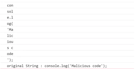
String splitting is a method by which an instruction is split every 3 or 4 characters and stored in a variable. All the individual pieces are then concatenated and then executed. This allows harmful pieces of code to get broken down, recombined at some other point and then executed. This is a particularly useful technique for hiding code.
Ex : return harmfulCode ; S t r in g 1 : r e t
S t r in g 2 : urn
Figure 8: Result of Instruction Substitution.
S t r in g 4 : rmf
S t r in g 5 : ulC
S t r in g 6 : ode
S t r in g 7 : ;
Recombined s t r i n g : return harmfulCode
To further explore the concept of Metamorphic JavaScript which is the aim of this project, we performed the splitting on the JavaScript code directly instead of performing them in the AST. This proved to be a simpler method rather than making changes in the syntax tree. More techniques can be implemented this way instead of parsing the code to AST and then back again with the drawback being that it could be detected by some antivirus.
Figure 9: Result of String Splitting.
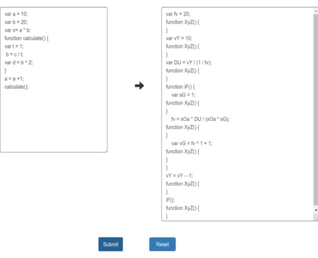
3.6 Dead Code Insertion
The last technique that we have tried to implement is Function Insertion. The main aim of Function Insertion is to insert dead code that does not affect execution. This creates morphed copies with different signatures to avoid detection. For imple-menting this technique, we explored ways for manipulating JavaScript code itself. We split the JS code on every occurrence of ";" character and insert dead code at that location. A simple implementation of dead code insertion is used. More complex mutations can be used such as randomizing the name of each function generated and inserting simple instructions inside each of the functions with randomized names. This would further morph the signature of the program.
CHAPTER 4
Assessing modification extent using Similarity Graphs 4.1 Rhino
In 1997, Netscape worked on a project that was aimed at creating a version of Netscape Navigator that was fully written in Java. The end product was called the ‘Rhino’ project, an open-source JavaScript implementation written in Java. This is now maintained by Mozilla. Rhino is used to compile JavaScript code to Java classes. It can primarily run in two modes - compiled and interpreted mode. The compiled mode is very useful as Rhino compiles JavaScript to a Java bytecode. This produced the best performance results, outdoing the C++ implementation of JavaScript with Just-in-time-compiling (JIT).
The Rhino engine consists of four parts namely Parser, Byte-Code generator, Interpreter and the JIT.
• Parser: The parser parses the JavaScript code and converts it to an AST. • Byte-Code generator: AST is then passed into the Byte-Code generator which
generates the bytecode.
• The Interpreter uses the output from the generator to convert the bytecode to machine code while using the JIT.
The output from the bytecode generator is needed for performing all the experi-ments. Once the AST is generated from the parser, the bytecode generator converts this to bytecode one block at a time. The sample output from the bytecode generator is shown below
JavaScript code : i n t a = 2 ; Byte code generated :
‘bipush’ is used to add a byte as an integer onto the stack which in this case is 2. ‘istore_0’ is used to store an integer in a local variable. The general format is istore_<n> where n can be 0, 1, 2, or 3 depending on the number of local variables. Anything greater than 3 is represented by the generalized opcode ‘istore’.
There are also limitations when it comes to using Rhino. The primary reason is, as compiling JS directly affects the load time of a page in the browser, Rhino can only compile small files [7]. To deal with this problem, a method is employed by Mangesh et al.[7] to compile a file of any length and disregard any optimization that Rhino inherently performs. The opcodes are extracted at compile time itself by writing the output to the console. This method saves the time of decompilation of the class file to extract the opcode sequence. However this method is not implemented as most of the files can be extracted using Rhino, including big files. The compilation process for an entire directory finishes in a matter of seconds. When the file is converted to a human readable format, most of the vital information is present in the file. It has a list of function calls to show the operations that take place and what value is stored in memory. Therefore the above method is deemed unnecessary.
To retrieve the output from the intermediate stage we perform extra steps shown in the next section.
4.2 Similarity Graphs
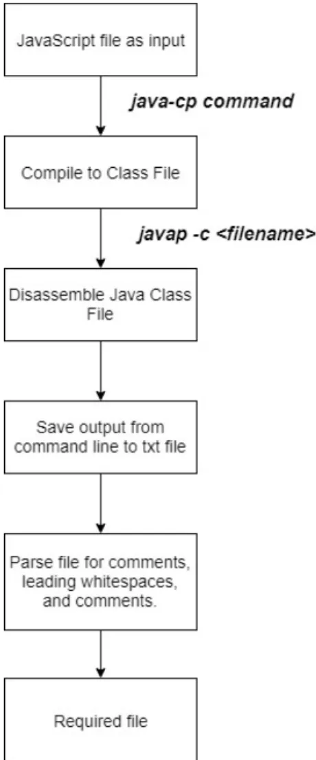
The method employed by Mishra et al. [2] will be used to assess the extent of metamorphism done by the engine and to compare two files of code. This program compares code at a bytecode level to quantify the degree of metamorphism after a file is passed through the metamorphic engine. To do this, the code needs to be converted to an appropriate form. Figure 10 illustrates the process mentioned below.
• The first step in the process is to compile the JavaScript file to a class file using Rhino. The following command is used.
Figure 10: Converting file to appropriate format
java −cp j s . j a r org . m o z i l l a . j a v a s c r i p t . t o o l s . j s c . Main • The next step is to disassemble the class file and convert it to human readable
language,
javap −c <filename >
• The output from the command line is saved as a txt file.
• The file is parsed using python to remove all the leading white spaces, function names, comments and the number preceding each instruction.
The java -cp command is used to compile the file from a JavaScript file to a class file and the javap command takes the class file as an input and gives us a more human readable file. A script is written to parse through a directory, retrieve all the JS files and perform the required operation thereby removing the manual work required for this process. A sample file in Figure 11 is shown below:
Figure 11: A sample file after converting to bytecode.
To compare two files we look to Mishra’s method. File X is the original code and File Y is the code that is passed through the metamorphic engine. The method put forward by Mishra consists of the following steps. Figure 12 illustrates the process mentioned below.
Figure 12: Assessing extent of metamorphism.[2]
• Given two pieces of code X and Y, X before the file is passed through the engine and Y after the metamorphism is done, the opcode sequences are extracted from each of the files. Redundant commands such as comments, blank lines, and such are removed from this sequence.
• The resultant file is an opcode sequence of length n and m wheren and m are
the number of opcodes in each file.
• Two opcode sequences are then compared by considering subsequences of three opcode. A match is found is all the three opcodes are similar regardless of their position in the subsequence. The coordinates (x,y) are marked on the graph where x is the opcode number of the first opcode of the three opcode sequence in program X and y is the opcode number of the opcode subsequence in program Y.
a n*m graph is obtained.
• If a line segment falls on the main diagonal of the graph, it means that the opcodes are at the same location in both the files. A line of the diagonal indicates that the match appear at different locations in the two files.
A number of experiments are run using this method to verify that the implemen-tation of JavaScript metamorphic techniques is effective.
CHAPTER 5
Support vector machines.
Support Vector Machines (SVM) proposed in the 1990s is a discriminative classifier. It is a supervised machine learning algorithm and a preferred model for classification as it has high accuracy with less computation power. It was mainly designed for pattern recognition but is also applied in many classification problems such as image, speech recognition, text categorization, and face detection.
Given training data which is labeled i.e each data belonging to a specific class, a SVM is capable of building a model that can predict the class of new test data. The main objective of a SVM is to find a separating hyperplane that can clearly classify data points. The hyperplane is a line dividing a plane into two parts where each data point falls into one category. Figure 13 below shows an example of the hyperplane. For a set of independent and identically distributed training sample
Figure 13: A HyperPlane [3]
The aim is to find a hyperplane represented as
𝑤𝑇.𝑥 +𝑏 = 0 (2)
which can be used to separate the two different samples accurately w is the weights vector, (x,y) is a set of training data, and b = -w.x0.
The optimal hyperplane is one that maximizes the distance from the hyperplane to nearest point of each class. This hyperplane is selected from a number of hyperplanes or the classifying patterns. The figure below 14 gives a basic idea.
Figure 14: Set of Possible Hyperplanes[3]
The dimension of the hyperplane is dependant on the number of features fed into the model. The model becomes more complex when the number of features exceeds 3. To build an SVM, Support vectors play a vital role. Support vectors are data points that are closer to the hyperplane and influence the position and orientation of the hyperplane.
Using Support vectors, we maximize the margin of the classifier. The bilateral blank area (2/ || w||) must be maximized to obtain the partition hyperplane and this is done by maximizing the weight of the margin. Formula 3 [3] is used to maximize the weight of the margin.
𝑀 𝑖𝑛Φ(𝑤) = 1/2||𝑤||2 = 1/2(𝑤, 𝑤) [3] (3) such that
𝑦𝑖(𝑤.𝑥𝑖+𝑏)>= 1 [3] (4) where w is the weights vector, and Φis the kernel function. The kernel function is used to map a pattern onto a higher dimension such that the pattern can become linearly separable. 1/2 is used in the formula as it is convenient for taking the derivative. 4 are the constraints to ensure that all instances are correctly classified. Maximizing the margin of the classifier is done to give better classification. Larger the margin, better is the classification of the model and thereby lesser percentage of error.
5.1 Implementation
For the implementation, a sequence is required as the input to the model. A significant amount of data pre-processing must be done to convert the files into the input format. The opcode sequence generated from Rhino in the previous step is used. The top 30 occurring opcodes have been used to create a dictionary. This dictionary will be used to convert the opcodes into symbols. This sequence of symbols will become the input to the SVM. A script file performs the following operation:
• The file is read line by line and stripped for leading and trailing white spaces to get each line.
• A check is done to see if each line starts with a digit since the output from Rhino is of the format ‘1:invokespecial’. This is done to remove function declarations and get only the opcode list.
• The line is split based on ‘:’ to get the opcode.
• Regular expressions are used to remove comments and any other extra charac-ters/symbols since Rhino generates comments in most lines.
symbol and stored.
The table below shows the contents of the dictionary.
Table 1: 30 most occurring opcodes and their symbols
Opcode Symbol Opcode Symbol
aaload 1 areturn 16 aload_0 2 ifne 17 invokespecial 3 aload 18 iload_3 4 getfield 19 putfield 5 ldc 20 aload_1 6 sipush 21 aload_2 7 bipush 22 tableswitch 8 putstatic 23 return 9 ireturn 24 iconst_0 10 aload_3 25 new 11 iload_1 26 dup 12 iconst_4 27 invokestatic 13 iconst_1 28 aconst_null 14 iconst_3 29 invokevirtual 15 ldc_w 30
A sample of the conversion is shown below. Bytecode :
aload_0 aload_1 return
i n v o k e s p e c i a l
Opcode sequence generated : [ 1 , 2 , 3 , 4 ]
This generates an array of variable length (depending on the size of the file). This is run for each of the input files. Once the opcode sequence is converted into symbols, this is then fed as the train data to the model and a label assigned to it. A
label ‘0’ is assigned if the file is a benign file and a label ‘1’ is assigned if the file is a malware file. The train and test data is split in an 80-20 ratio. The SVC classifier is used in this model, fitted and can then be used to predict against the test data. The parameters for the SVC are mostly the default values. Parameter tuning done for this implementation is, the kernel is set to ‘rbf’, gamma is set to ‘scale’ and the max_iter is set to -1. A python script is written to create the model.
To evaluate the classifier output from the model, the Receiver Operating Charac-teristic (ROC) is used. The Y axis of a ROC curve is the true positive rate (TPR) and the X axis is the false positive rate (FPR). The top left corner of the plot i.e FPR of zero, is the ideal point. While this is not possible in most cases, it does mean that a larger AUC is better [19]. The ‘steepness’ of ROC curves is also important since it is ideal to maximize the true positive rate while minimizing the false positive rate[19]. ROC can be also be used for multi-label classification. This is calculated by comparing the y_test and y_score.
y_score = c l a s s i f i e r . f i t ( X_train , y_train ) . decision_ func t io n ( X_test )
The roc curve is plotted by calculating the area of the curve of the false positive rate and the true positive rate.
In recent years, Hidden Markov models have had great success in classifying malware. In this implementation, SVM’s are chosen over Hidden Markov Models to classify data as malware or benign due to a vital reason. In the case of the HMM, the data points fed to the model consists of a two dimensional array where each row corresponds to the opcode sequence of one file. The limitation is that the files fed to the HMM is considered as one file instead of considering each file separately i.e
How HMM’ s c o n s i d e r s i t : [ f i l e 1 ]
Thus the HMM calculates the probability of one symbol appearing after the next and not classifying the malware based on the opcode sequence in each malware file. Implementing a Hidden Markov Model that accepts a two dimensional array is not straight-forward and requires a lot of mathematical calculations. This makes SVM to be the more suitable algorithm in this case.
CHAPTER 6 Experiments and Results
This chapter covers all the experiments, files used and the results from each of the experiments mentioned below. The methods experimented with are listed below
• Metamorphic Engine • Similarity Graphs • HMM/SVM.
The metamorphic engine works on the JavaScript while the similarity graph and the model on the opcode/opcode sequences. Benign and malware files are in JavaScript and then passed through the engine. This is converted to opcodes using Rhino. Opcode sequences are then extracted from each of the files using bash script files. All of the experiments are performed on a laptop with the following system configurations listed in Table 2.
Table 2: System configuration’s
Model Lenevo
Processor Intel(R) Core(TM) i7-6700HQ CPU
@ 2.60GHz (8 CPUs), 2.6GHz
RAM 16GB
System Type 64-bit
Java Compiler Java8
Host Operating System Windows 10
Guest Operating System Ubuntu 16
The malware files are stored/extracted on a Ubuntu environment in an Oracle VM VirtualBox. This is done as a precaution in case the malware somehow affects the system. Snapshots also allow you to go back to a previous system point.
For the dataset, the files used consist of benign and malware files. The breakup is shown in Table 3.
Table 3: Breakdown of benign files list
Source File Number of Files Lines of Code (LOC)
jQuery uncompressed 1 10364
Angular JS 10 7320
Popper.js 8 6230
3JS 10 8100
YUI Library files 20 9000
Cassandra 10 1850
Total 59 42864
year of 2017. A variety of malware totaling 50 is selected and used for the malware samples. 60 different JavaScript files from different libraries are used as the benign set.
6.1 Similarity Graphs:
For the similarity graphs, different experiments have been performed and the results have been listed down below. The advantage of similarity graphs is that it creates a visual representation of the difference between the two pieces of code. A match across the diagonal indicates that the file is similar in the same location i.e the metamorphic engine does not cause enough change to the code. A match away from the diagonal indicates that the file is similar in different places of the code. When a steady diagonal is not present in the graph, it shows that the engine is performing well and the resultant code from the metamorphic engine is completely different while remaining functionally equivalent.
6.1.1 Sliding windows
The first experiment conducted is the sliding window experiment. Mishra [2] assumes a sliding window of 3 opcodes to be ideal. This is put to a test as an opcode sequence of 5 could also result in better output. If a match does not occur for a length of 5, there is definitive proof that metamorphic techniques are used and that there
is a significant difference. The similarity graphs were run against different sliding windows (length of 1,2, 3 and 5) of the opcode sequences and observed.
Figure 15: Sliding window of 2.
From the figures 15, 16, and 17, it becomes clear that bigger the sliding window is lesser are the number of matches between the two opcode sequences. From figure 15, it is clear that there are too many unwanted matches that occur between the two opcode sequences due to the small size of each window. A sliding window of ‘3’ and ‘5’ is more promising in that regard and can be used for the experiments. From the figures 16 and 17, the number of random matches are drastically lesser. A sliding window of ‘3’ seems to be the ideal number to perform experiments but a number of ‘5’ could also be used for future experiments.
Figure 16: Sliding window of 3.
Figure 17: Sliding window of 5.
6.1.2 Experimenting with each of the techniques
The similarity graph is used to assess the strength of each technique in the metamorphic engine. An experiment is run to see which combination of techniques
yield the best result. While all the five techniques is the best approach, it would be interesting to see how to mix and match the techniques for future implementations. A sliding window of ‘3’ is chosen for all the experiments shown below.
Figure 18: A file matched against itself.
The above figure shows the same file matched against itself without going through the metamorphic engine. A clear diagonal indicates that the opcode sequences are present at similar locations in each of the files.
Graph 1 indicates when sequential matches are done i.e window (1,2,3) followed by window (4,5,6) are compared. Graph 2 indicates when a sliding window of 3 i.e window (1,2,3 ) followed by window (2,3,4) is used to check the two files. Both methods are
implemented purely for experimentation.
Figure 19 shows the degree of metamorphism performed by the instruction reorder-ing technique. From the diagonal, it is clear that the degree of metamorphism that it performs is very less from the opcode sequences extracted. There is a small break in the
Figure 19: Instruction Renaming.
instruction names are present in a function in the end called ‘getParamOrVarConst’. Thus the change appears only towards the end of the diagonal. While this break is not significant, it can be effective for bigger files.
Figure 20 shows the degree of metamorphism done by the engine performing only Instruction Reordering. From the figure, it is clear that this technique performs very less change. Since we swap two independent instructions within the same scope and compare a sliding window of 3 opcode sequences in the similarity graphs in any order, the change that appears is very minimal. The break occurs when instructions that are independent, in the same scope, and do not occur sequentially are present in the program. Thus this technique is not very effective while performing metamorphism. A lower value of the sliding window might provide better results.
Figure 21: Instruction Substitution.
Figure 21 shows the degree of metamorphism done by the engine performing only Instruction Substitution. Similar to Figure 20, the changes by Instruction Substitution is minimal.
Figure 22 corresponds to dead code insertion done by the metamorphic engine. This technique creates the most metamorphic functionally equivalent code. Dead
Figure 22: Dead Code Insertion.
From the graph, it is apparent that the output from the engine is nothing like the initial code. Thus this technique is very effective at altering the structure of the code and thereby the signature.
6.1.2.1 Dead code vs All other techniques.
From the above graphs, it is very apparent that dead code insertion offers very promising results. This is compared to an engine that performs all the other techniques. When comparing the techniques, the metamorphism performed by dead code is much better than all the other techniques combined. This implementation of dead code inserts the code wherever semicolons are present and appends the rest of the body to it. While this implementation might increase the amount of memory required for the program also making it more visible to the user, this does offer more promise when it comes to changing the signature of the code. Also when inserting dead code, care must be taken because if the malware writer is too reliant on dead code, there are
(a) All the other techniques combined
(b) Dead Code
6.2 SVM:
A variety of experiments were run with SVM during the detection phase of this project. The dataset consists of benign files taken from various sources and the malware files are taken from the 40000 JavaScript collection samples from GitHub. Table 4 shows the number of files that are used in the training and testing phase of the SVM.
Table 4: Number of Files to the SVM Source File Number of Files
Benign Files 45
Malware 40
Total 85
The above files are split roughly in a 90-10 ratio to get the training and test data. Table 5: Training and Test data split
Data Number of Files
Training Data 75
Test Data 10
Total 85
Data pre-processing:
The following steps are used to get the data that is fed to the SVM. • The JavaScript file is passed through Rhino to get the class file.
• java-p is then used to get a human-readable format to work with. A python script then converts the file to an input for the SVM.
• The file is read line by line and stripped for leading and trailing white spaces to get each line.
• A check is done to see if each line starts with a digit since the output from Rhino is of the format ‘10:return’. This is done to remove function declarations and get only the opcode list.
• The line is split based on ‘:’ to get the opcode.
• Regular expressions are used to remove comments and any other extra charac-ters/symbols since Rhino generates comments in most lines.
• If the opcode matches the key in the dictionary, the opcode is converted into a symbol.
• A length of 500 opcodes is chosen as an ideal point for the length of the opcode sequences.
• If the opcode length is more than 500, the first 500 opcodes are used to represent the file. If the opcode length is less than 500, a ‘other’ symbol is used to fill the array with a symbol. In this case, ‘45’ is taken as that symbol.
• This output is then written to a file.
A sample is shown below of a row generated from the python script that converts the byte code into symbols. The sample below consists of the first 30 symbols of a file.
[ 2 , 2 , 10 , 9 , 12 , 2 , 9 , 2 , 6 , 7 , 12 , 14 , 16 , 6 , 2 , 6 , 7 , 25 , 16 , 2 , 6 , 7 , 25 , 16 , 10 , 24 , 16 , 10 , 24 , 24]
6.2.1 Experiment1: Opcode Length
The first factor to decide on is the opcode length for each file. Since the length of each file varies, an ideal length parameter must be decided. This is done such that smaller files can append an ‘other’ symbol to fill up the opcode sequence to make each row of the array of equal length. The first experiment was conducted using the length value of 250. The data set taken for this experiment consisted of 50 files which can be broken down into 20 malware and 30 benign files. The following figure shows the output from the experiment.
Figure 24: ROC curve for Experiment 1.
size of the dataset. The main reason for this is that the length of the opcode sequence taken for each file is insufficient for the model to draw conclusions for classification. Also, the size of the dataset is small for this experiment as the data preprocessing required to obtain the converted opcode sequence is very time consuming and tedious even with the help of scripts to automate the process.
Another solution could be to set the optimal length to be the length of biggest opcode sequence and pad all the other files with the ‘other’ symbol. But the drawback of this method is that since the file size varies quite often, many files end up with more padding rather than the actual file.
A length of 500 gives the best accuracy in classification. Figure 25 shows that this length is an ideal limiter for the opcode sequence.
6.2.2 Experiment 2: Parameter tuning for SVC
Some of the important parameters that have been experimented with have been explained below.
The kernel parameter decides the type of hyperplane that splits the data. The parameter that can be used is ‘linear’, ‘rbf’, and ‘poly’. Linear is not selected as this will use a linear hyperplane to separate the data. Rbf is chosen since a non-linear hyperplane is used. Gamma is a parameter that is used for non-linear hyperplanes. The training data set is exactly fit given higher a gamma value. The gamma parameter is set to ‘scale’ as the ‘auto’ parameter is now deprecated and setting it to this value means that no value is passed. The scale parameter uses the formula 1/ (n_features * X.var()) to determine the value of the kernel coefficient. These parameters are used in 25 The final parameter is max_iter which is set to ‘-1’i.e the number of iterations as no limit. Setting a limit on the maximum number of iterations results in the accuracy dropping drastically to 50%.
Other parameters such as ‘C’ used the default value that is passed to the SVC. The figure 25 shows that the model is highly accurate and efficient when it comes to detecting malware based on the opcode sequence. This model is used to test if SVM’s are capable of detecting any metamorphic operations performed on benign / malware files. By detecting the changes at a byte code level and analyzing the opcode sequences will help finalize how efficient metamorphic techniques are.
This implementation of SVM has a higher accuracy than existing implementations of SVM for malware detection. Existing implementation using SVM by Ranveer et al. [18] achieved a 92% accuracy for opcode based malware detection and Santos et al.[17] achieved a TPR of 0.95 for malware detection. The implementation in this project has a better accuracy for a dataset of the same size. Thus to test metamorphic
Figure 25: Ideal parameters that give best accuracy. code, a powerful detection algorithm with a very high accuracy is used.
6.2.3 Experiment 3: Adding new classes to the classification.
This section experiments with using benign metamorphic code to make the problem harder. In this experiment, an extra class is added which represents benign metamorphic code.
Table 6: Classes and their representation
Class Label
Benign file 0
Malware file 1
Benign Metamorphic file 2
A file consisting of benign metamorphic code is a benign file that is passed through the metamorphic engine and morphed. If the SVM is capable of separating the data into the third class accurately, a conclusive method is now found to detect the presence of these effective metamorphic techniques. The same preprocessing is done to get the
data in the appropriate form.
Table 7: Number of Files to the SVM
Source File Number of Files
Benign Files 45
Malware Files 40
Benign Metamorphic Files 45
Total 130
Table 8: Training and Test data split
Data Number of Files
Training Data 110
Test Data 20
Total 130
Table 7, 8 highlights the breakdown of the input files and the split of the train-test data. 45 benign files are passed through the metamorphic engine and added to our train data. The output from the model is shown below in Figure 26. ‘micro-average’ and ‘macro-average’ also tell us how to model performs by giving the average statistic information of the classification. The ‘macro-average’ in the figure is the calculated metrics (true positive rate, false positive rate) for each label which is then used to find the mean. The ‘micro-average’ is the collective metrics for all labels globally to compute the average [19]. For most multi-class classification, micro-average is preferred in case of class imbalance.
The SVM is capable of classifying benign metamorphic code with an accuracy of 86%. An area under the curve (auc) value of 0.8 and macro average (as there is no dataset imbalance) of 0.90 is obtained for benign metamorphic class meaning that the model is capable of decisively classifying the file. Thus the opcode sequence can be fed to the Support Vector Machine to detect metamorphic code with reasonable
Figure 26: Accuracy result for SVM
class is taken into consideration as the number of files used in the dataset is less. This drop in accuracy is acceptable as an extra class is added. This stands to prove that SVM can be used to detect metamorphic code with reasonable accuracy.
CHAPTER 7
Conclusion and Future Work
The aim of this project was to explore and test the various metamorphic techniques using JavaScript and assess how effective each of the techniques are when it comes to changing the structure of the code. Rhino is used to compile JavaScript files to class files which can then be converted into bytecode and thereby extracting the necessary opcodes. These opcode’s can then be used for all the further experiments. Similarity graphs was implemented to visualize how much the code morphs by using these techniques. It is found that Dead code was particularly effective when it comes to morphing the code. While the other techniques do show promise, the signa-ture does not vary as much. This project also explains why SVM’s would be a better classification algorithm over HMM’s when observing the opcode sequence’s. From the experiments, we can conclude that SVM’s can classify malware and detect metamor-phic code with a high degree of accuracy. When classifying malware, 98% accuracy is observed and when when detecting/classifying metamorphic benign files, 86% accuracy is observed. Given that the model is capable of detecting metamorphic benign files, it will also be able to detect metamorphic malware. A more advanced version of SVM would be able to detect almost any metamorphic malware techniques used in the future. Future work for this experiment can be to test SVM’s against metamorphic malware’s techniques such as Transcriptase and Advanced Transcriptase. These techniques have proved to be very hard to detect in previous research papers. Given how promising the results are from the experiments performed, SVM should be able to classify advanced malware techniques. To improve accuracy of the model, the size of the dataset could be drastically increased to around 1000/2000 files. A lot of time
LIST OF REFERENCES
[1] V. Naidu and A. Narayanan, ‘‘A syntactic approach for detecting viral polymor-phic malware variants,’’ 03 2016, pp. pp 146--165.
[2] P. Mishra, ‘‘Taxonomy of uniqueness transformations,’’San Jose State University, Master’s Projects, Department of Computer Science, 2003.
[3] A. Pradhan, ‘‘Support vector machine-a survey,’’International Journal of Emerg-ing Technology and Advanced EngineerEmerg-ing, vol. 2, no. 8, pp. 82--85, Aug 2012.
[4] Y. Ling and N. F. M. Sani, ‘‘Short review on metamorphic malware detection
in hidden markov models,’’ International Journal of Advanced Research in
Computer Science and Software Engineering, vol. 7, pp. 62--69, 02 2017.
[5] J. Lewis, ‘‘Economic impact of cybercrime, no slowing down,’’ Feb 2018. [Online]. Available: https://www.mcafee.com/enterprise/en-us/assets/reports/restricted/ rp-economic-impact-cybercrime.pdf
[6] B. Bashari Rad, M. Masrom, and S. Ibrahim, ‘‘Camouflage in malware: From
encryption to metamorphism,’’ International Journal of Computer Science And
Network Security (IJCSNS), vol. 12, pp. 74--83, 01 2012.
[7] M. Musale, T. H. Austin, and M. Stamp, ‘‘Hunting for metamorphic
javascript malware,’’ Journal of Computer Virology and Hacking Techniques,
vol. 11, no. 2, pp. 89--102, May 2015. [Online]. Available: https:
//doi.org/10.1007/s11416-014-0225-8
[8] D. Lin and M. Stamp, ‘‘Hunting for undetectable metamorphic viruses,’’Journal in Computer Virology, vol. 7, no. 3, pp. 201--214, Aug 2011. [Online]. Available:
https://doi.org/10.1007/s11416-010-0148-y
[9] P. Ször and P. Ferrie, ‘‘Hunting for metamorphic,’’ in In Virus Bulletin Confer-ence, 2001, pp. 123--144.
[10] F. D. Troia, C. A. Visaggio, T. H. Austin, and M. Stamp, ‘‘Advanced transcriptase for javascript malware,’’ in2016 11th International Conference on Malicious and Unwanted Software (MALWARE), Oct 2016, pp. 1--8.
[11] N. Idika and A. P. Mathur, ‘‘A survey of malware detection techniques,’’ Purdue University, vol. 48, 2007.
[12] A. Kalbhor, T. H. Austin, E. Filiol, S. Josse, and M. Stamp, ‘‘Dueling hidden markov models for virus analysis,’’ Journal of Computer Virology and Hacking Techniques, vol. 11, no. 2, pp. 103--118, 2015.
[13] W. Wong and M. Stamp, ‘‘Hunting for metamorphic engines,’’Journal in
Com-puter Virology, vol. 2, pp. 211--229, Nov 2006.
[14] W. Wong, ‘‘Analysis and detection of metamorphic computer viruses,’’ San Jose State University, Master’s Projects, Department of Computer Science, 2006.
[15] D. Bruschi, L. Martignoni, and M. Monga, ‘‘Detecting self-mutating malware using control-flow graph matching,’’ in Detection of Intrusions and Malware & Vulnerability Assessment, R. Büschkes and P. Laskov, Eds. Berlin, Heidelberg:
Springer Berlin Heidelberg, 2006, pp. 129--143.
[16] M. Mohammed, ‘‘Zeroing in on metamorphic computer viruses,’’ Master’s thesis, Univ. of Louisiana at Lafayette, 2003.
[17] I. Santos, F. Brezo, X. Ugarte-Pedrero, and P. G. Bringas, ‘‘Opcode sequences as representation of executables for data-mining-based unknown malware detection,’’ Inf. Sci., vol. 231, pp. 64--82, May 2013. [Online]. Available:
https://doi.org/10.1016/j.ins.2011.08.020
[18] S. Ranveer and S. R. Hiray, ‘‘Svm based effective malware detection system,’’ 2015.
[19] F. Pedregosa, G. Varoquaux, A. Gramfort, V. Michel, B. Thirion, O. Grisel, M. Blondel, P. Prettenhofer, R. Weiss, V. Dubourg, J. Vanderplas, A. Passos, D. Cournapeau, M. Brucher, M. Perrot, and E. Duchesnay, ‘‘Scikit-learn: Machine learning in Python,’’ Journal of Machine Learning Research, vol. 12, pp.
2825--2830, 2011.
[20] H. Petrak, ‘‘Javascript malware collection,’’ https://github.com/HynekPetrak/ javascript-malware-collection, 2017.