Improving Electroencephalography-Based Imagined Speech Recognition with a Simultaneous Video Data Stream

Computer Science and Computer Engineering

Undergraduate Honors Theses Computer Science and Computer Engineering

5-2016

Improving Electroencephalography-Based

Imagined Speech Recognition with a Simultaneous

Video Data Stream

Sarah J. Stolze

Follow this and additional works at:http://scholarworks.uark.edu/csceuht

Part of theArtificial Intelligence and Robotics Commons,Graphics and Human Computer Interfaces Commons, and theOther Computer Sciences Commons

This Thesis is brought to you for free and open access by the Computer Science and Computer Engineering at ScholarWorks@UARK. It has been accepted for inclusion in Computer Science and Computer Engineering Undergraduate Honors Theses by an authorized administrator of ScholarWorks@UARK. For more information, please [email protected].

Recommended Citation

Stolze, Sarah J., "Improving Electroencephalography-Based Imagined Speech Recognition with a Simultaneous Video Data Stream" (2016).Computer Science and Computer Engineering Undergraduate Honors Theses. 38.

Simultaneous Video Data Stream

An Undergraduate Honors College Thesis

in the

Department of Computer Science Computer Engineering

College of Engineering

University of Arkansas

Fayetteville, AR

by

1. Introduction 1 1.1 Problem 1 1.2 Objective 2 1.3 Approach 2 2. Background 4 2.1 Key Concepts 4 2.1.1 Electroencephalography Devices 4

2.1.2 Pattern Recognition Techniques 6

2.2 Related Works 7

3. Design and Experiments 9

3.1 Hypothesis 9

3.2 High Level Experiment Design 9

3.3 Data Set Collection 9

3.4 Data Processing 12

3.5 Algorithms 14

4. Results and Analysis 15

4.1 Methodology 15 4.2 Results 15 4.3 Analysis 18 5. Conclusions 20 5.1 Summary 20 5.2 Potential Impact 20 Data Appendix 21 References 26

INTRODUCTION 1.1 Problem

Imagined speech (unspoken speech, silent speech, or covert speech) is the process by which one thinks about a word, or “hears” the word in one’s head, in the absence of any

vocalization or physical movement indicating the word. There exists evidence that it is possible for imagined speech information to be captured and interpreted by a machine learning classifier [1]. In order to collect data pertaining to imagined speech, a Brain-to-Computer Interface (BCI) must be implemented to provide silent communication abilities directly between the two entities. One of the most popular methods for interfacing directly between a human brain and a computer is through electroencephalographic signals [1].

Electroencephalography (EEG) devices provide a non-invasive mechanism for measuring electrical signals transmitted near the surface of the brain. These devices can be used to facilitate unspoken speech recognition via the implementation of a brain-to-computer interface (BCI) to communicate a user’s thoughts directly, effortlessly, rapidly, and privately to a machine. Such a system might facilitate a host of applications including prostheses control, immersive command of remote robots, integration with wearable computing, or telepathic note-taking [11].

Researchers have created models capable of achieving 70 - 90% predictive accuracy in recognizing patterns in EEG data [13, 14, 15]; however, the accuracy of current methods for unspoken speech recognition is not yet sufficient to enable fluid communication between humans and machines. The ability to achieve a higher predictive accuracy is hindered by a variety of obstacles standing in the way of implementing a BCI with an EEG device. This project seeks to analyze a unique method for addressing the following problems with imagined speech

recognition via EEG devices: low signal-to-noise ratio, uncertainty as to the content in EEG signals, and scarce availability of training data.

1.2 Objective

The objective of this project is to improve a classifying algorithm's capacity to facilitate unspoken, or imagined, speech recognition by collecting and analyzing a large dataset of simultaneous EEG and video data streams.

1.3 Approach

This project examines the validity of the hypothesis that obtaining a large volume of data with corresponding high-dimensional EEG and video features will allow a classifier to more effectively extract information from EEG signals. To do so, it is necessary to minimize the effects of inherent limitations for current methods in imagined speech recognition. The limitations addressed in this project are noise, uncertainty in EEG signals, and insufficient quantities of training data. Rather than investigate new approaches in terms of classifying and data processing algorithms, this project explores the effects of analyzing concurrent sources of information such as video components and noise-inducing EEG samples. It is proposed that adding such complexity to a classifying algorithm’s input will enhance its ability to extract features from EEG signals as well as information regarding the subject’s environment.

To address the low signal-to-noise ratio, the data collection process includes the measurement of subject’s EEG signal responses to certain known stimuli that generate particularly noisy signals. Information extracted from the data collection process includes a control group with measurements that represent noise-inducing actions such as a user’s physical movement, eye blinking, or facial expression [1, 16]. Other researchers have successfully trained learning algorithms to recognize common sources of noise like eye movements and blinks in

order to remove noisy components from the EEG signal [17, 18]. However, this project differs in that the classifier will be presented with the complete digital camera feed, suggesting the ability to detect additional sources of noise. Because the classifying algorithm will learn from the video stream, it may be able to detect other features that have not yet formally been classified as causes of noise, like breathing motions or muscles used to contribute to facial expressions. To further separate the signal from the noise, data is recorded to measure each individual subject’s neutral state of thought, where they were instructed to clear their minds of any particular thought. Understanding a subject’s EEG data and base facial position in a neutral state is expected to enhance the classifier’s ability to understand and separate the noise from the signals relevant to imagined speech recognition.

2. BACKGROUND 2.1 Key Concepts

This section describes the input components utilized in this project, EEG and video data streams. Secondly, it describes the pattern recognition techniques used for consistent data classification.

2.1.1 Electroencephalography Devices

Electroencephalography (EEG) devices measure and amplify spontaneous electrical activity of the brain. The human brain is composed of billions of neurons which emit electrical charges that eventually reach the surface of the scalp. Because the electrical potential generated by individual neurons is too subtle to be detected separately, the measurements from EEG devices reflect the summation of the synchronous activity generated by millions of neurons that have a similar spatial orientation [19].

Although EEG recordings are frequently used in medical and research environments, it remains largely unknown which cortical processes are represented in EEG signals and which are not [5]. One major reason for this lack of association between EEG output and cortical processes is the inherently low signal-to-noise ratio of EEG signals. EEG data is notoriously obfuscated by erroneous electrical signals with non-cerebral origins. These problematic electrical signals, also known as artifacts, are generally quite large relative to the size of amplitude of the cortical signals. The most common sources of these artifacts often stem from electromyographic (muscle activation) signals, or electrocardiographic (cardiac) signals. The limitations of EEG signals addressed in this project are listed below in order of magnitude of effect. Progress in understanding the contents of EEG signals depends on finding ways to address these known complicating factors.

Noise: The most prominent factor inhibiting the classification of EEG data for the task of imagined speech recognition is an inherently poor signal-to-noise ratio (SNR). Even minute electromyographic (or muscle) movements, such as eye blinking, facial expressions, and neck motions induce comparatively dominant signals that overwhelm and obscure the signals

produced from the brain. Additionally the brain also produces many signals that are irrelevant to imagined speech recognition [20].

Uncertainty: Classifying high-dimensional EEG data is a difficult task, because it is not known how imagined speech manifests itself within EEG data [1]. Where classification with static systems is a very mature field, classification with systems involving state and change over time in multiple dimensional space is a problem that requires more specialized expertise. Some efforts to classify EEG have included spectral decompositions of the signal in the features used to train the classifier [18, 26]. This gives the classifier an ability to discriminate periodic temporal patterns within a window of time; however, since the brain is a dynamic system with non-periodic signals, it is necessary to model it as a dynamic system [27, 28].

Limited Training Data: As a result of the extremely low signal-to-noise ratio in EEG signals, effective machine learning algorithms need large data sets to isolate the valuable

components from the noise. Such large data sets are cumbersome to produce due to the need for specialized hardware equipment and deliberate human attention to collect valid labeled training samples. Additionally, when EEG data is collected, it is not guaranteed to be consistent or complete. As a result of the inconsistent nature of human focus and attention span, it is also difficult to assure that data samples are accurately labeled. Because the nature of human attention span is unpredictable and volatile, it cannot be guaranteed that a subject is actually thinking clearly about the specified word or idea, nor can we accurately measure the human subject’s

level of focus or level of distraction during the data collection process. Until a better approach for gathering data is realized, imagined speech recognition with EEG devices is limited to be a “small data” problem because of the practical difficulty in assembling sufficiently large data samples.

2.1.2 Pattern Recognition Techniques

In order to extract valid feature information from high dimensional EEG signals, it is necessary to use sophisticated machine learning and pattern recognition algorithms. Machine learning techniques can already be used to recognize a small set of thought-based commands within EEG signals [1, 6]. Within the research community, supervised learning techniques are a fairly mature field, and yet the best-performing supervised learning algorithms are only able to extract high-level commands from EEG signals with limited vocabulary size, usually between 2 to 5 words [1, 15, 21].

One supervised learning algorithm that has attracted wide usage for EEG feature

extraction purposes is an Artificial Neural Network (ANN) [22, 23]. ANNs are loosely inspired by the human brain. Due to their structural parallels with biological neural networks, ANNs are a common choice of model for learning to recognize patterns in EEG signals. When implemented correctly, ANNs have proven to be well suited for this task; however, proper implementation of ANNs requires specialized training techniques [24]. Among different flavors of ANNs, deep ANNs and convolutional ANNs have proven to be most effective at classifying EEG data, but in addition to complex training techniques, these types of ANNs are notorious for being extremely computationally expensive [23, 24].

The primary focus of this research is not to propose a more effective classifier algorithm specifically designed to process EEG data, but rather to demonstrate that presenting a

well-known classifier with compatible sources of information, such as video components and noise-inducing EEG samples, will enhance the algorithm’s ability to extract valid features from EEG signals. Therefore, despite the potential benefits of using an ANN, I opted to use a much simpler pattern recognition algorithm: random forest (RF). A RF combines multiple random decision trees to form a bagging ensemble. While random forests are computationally inexpensive and easy to implement, the algorithm is known to be vulnerable to overfit when training on noisy data sets [10]; however, in this project the high dimensionality of the input dataset should help mitigate the risk of RF overfitting to the noise in EEG signals. Contemporary research suggests that the RF algorithm outperforms a variety of other prominent machine learning algorithms in terms of ability to accurately analyze EEG data [9]. In addition to its competitive predictive accuracy in EEG signal classification, the RF algorithm also boasts a high computing

performance and is exponentially faster and easier to train over more complex models such as ANNs [9, 10].

2.2 Related Works

Almost a decade ago, Suppes et al. conducted preliminary research into the potential for unspoken speech recognition using both EEG and MEG (magnetoencephalography) data. The findings from these experiments confirmed the potential for whole-word recognition. However, the results were highly dependent on subject and experimental conditions. With predictive accuracy rates ranging from 97% to barely above chance, the authors recognized the need for substantial improvement in terms of generalizing imagined speech classification techniques [25].

As discussed in the previous section, many researchers have achieved relative success in extracting EEG features using specialized Artificial Neural Networks (ANNs). Researchers in Canada were able to train a deep-belief network to classify phonological categories combining

acoustic, facial and EEG data and obtain predictive accuracies of over 90% [20]. Unlike other models, the experiments detailed in this paper used leave-one-out cross-validation which indicates that the results are both subject-independent and generalizable. This suggests that generalized artifacts related to speech production are in fact present in EEG data and that these artifacts can be extracted when a learning algorithm is presented with accurate knowledge of state.

Recently a rudimentary BCI enabled a paraplegic man to execute the opening kick at the 2014 World Cup using a robotic suit [7]. However, this system relied heavily on other

technologies for important components, like maintaining balance, where the EEG signal was simply used to obtain basic high-level commands from the user. This system required extensive prior training of the user as well as the device and significant mental concentration on behalf of the user [8]. This event shows how the development of BCIs are still in the state of infancy and thus require more research in order to exhibit characteristics of a more complete BCI. Highly desirable BCI characteristics include predictive accuracy in the range of 95% or better,

recognized vocabularies of 10 or more words, and less cumbersome training processes for both the user and the machine. Clearly there are many aspects of BCIs and imagined speech

3. DESIGN AND EXPERIMENTS 3.1 Hypothesis

We hypothesize that supplementing EEG data with simultaneous video data will allow for a classifying algorithm to more effectively facilitate imagined speech recognition.

3.2 High Level Experiment Design

For the experiments conducted, a uniquely comprehensive dataset was collected to test the hypothesis that the addition of video data will enhance a machine’s ability to classify EEG signals. Volunteer subjects wore a commercial EEG headset in front of a digital web camera. During the test, the subjects were asked to imagine a specific word or feeling (label). The subjects responded to a set of uniform verbal cues describing the set of labels as well as the desired individual label to imagine. The data was then processed in order to minimize the effects of irrelevant signal activity, or noise. Additionally the data was processed to minimize its volume while still maintaining the core “information” in the data. The condensed dataset was created by dropping irrelevant information from the EEG device and applying principal component analysis (PCA) to the video stream data. Once the data was processed and assembled into the correct format, cross-validation using a random forest algorithm was performed on the control group of EEG signals alone and on the hypothesis group consisting of both EEG and video data. The predictive accuracy measurements obtained from the cross-validation experiments were used as metrics to evaluate the success of the hypothesis.

3.3 Data Set Collection

Simultaneous EEG readings and digital video streams were recorded for 20 different volunteer subjects. For each subject, the data represents a uniform set of words (or labels) representing imagined speech, including a control group to classify causes of EEG signal spikes

such as eye blinking. The EEG data was recorded with a commercial 14-channel Emotiv EPOC Model 1.0 headset, which operated at a rate of 128 samples per second. The digital video stream was recorded with a standard 1.3 Megapixel web camera with a framerate of 30fps.

In order to maximize consistency, the data collection process was standardized based on the following outline for each individual subject. For every part described in the tables below, the number of samples per word indicated how many 1-second samples were taken for each word, e.g. 5 samples per word means 5 seconds of simultaneous EEG and video recordings. The verbal queue was the general explanation used to provide consistency in the instructions for test subjects during the data collection phase. After initiating the appropriate verbal queue, the proctor allowed the subject a few seconds to stabilize focus on the correct label. Once it was observed that the subject was sufficiently focused, the proctor collected the appropriate number of 1-second data samples from synchronized EEG and video streams. The proctor

simultaneously recorded data from both the EEG headset and the video camera every time a character on the keyboard is pressed. A variety of different characters were assigned to each label representing an imagined word or phrase. There were four distinct label groupings during the test: Control, Feelings, Random, and Directions. Each is described in detail by the tables below.

Figure 1: Table description of Control label data acquisition.

Group 1: Control

Word # of Samples Verbal Queue

[N] neutral 5 “Try to empty your mind, and try not to focus on anything.”

[M] movement 10 “Make small facial and body movements.”

[K] blink 5 “Blink as you normally would.”

Figure 2: Table description of Feelings label data acquisition.

Group 2: Feelings Samples per word: 2

Verbal queue: “Imagine how it feels to…” [1] stub your

toe

[3] make a mistake [5] ace an exam [7] be

disappointed

[9] smile [2] fall down [4] grab a cactus [6] laugh w/ friends [8] get sick [0] be relieved

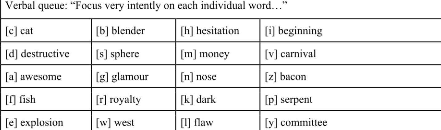
Figure 3: Table description of Random label data acquisition.

Group 3: Random Words

Samples per word: 2

Verbal queue: “Focus very intently on each individual word…”

[c] cat [b] blender [h] hesitation [i] beginning

[d] destructive [s] sphere [m] money [v] carnival

[a] awesome [g] glamour [n] nose [z] bacon

[f] fish [r] royalty [k] dark [p] serpent

[e] explosion [w] west [l] flaw [y] committee

Figure 4: Table description of Directions label data acquisition.

Group 4: Directions Samples per word: 10

Verbal queue: “Focus on the feeling of yourself moving in one particular direction...”

[F] forward [R] right

[B] backward [U] upward

Due to dependence on humans both as test subjects and proctors in this experiment, the information contained in this dataset is not guaranteed to be completely uniform. It is possible that during the data collection process, a subject responded to some external stimuli and lost focus during the test, thus skewing the association between the data and the label. Perhaps certain subjects were more focused and engaged than others. Additionally, there was one instance where the proctor accidentally collected one too few data samples.

Though there are a few inconsistencies present due to human involvement, the dataset offers a unique representation of simultaneous EEG and digital video data. Currently it is believed that this is the only comprehensive EEG and video dataset of its kind. Therefore to further science, this dataset will be published online at mldata.org and made available for other researchers and data enthusiasts. The researchers will release the collected dataset to allow the research community to better understand the important features and patterns contained within complex and high-dimensional EEG data.

3.4 Data Processing

Appropriate processing was necessary to standardize the dataset and eliminate

inconsistencies that may have skewed results. The raw data was also stripped down to allow for more efficient processing without compromising the integrity or the content of the data. Data processing was also necessary to prevent the classifier from accessing information that would allow it to “cheat,” or pick up on arbitrary patterns (like timestamps or sample counters) in the data that were not related to imagined speech recognition.

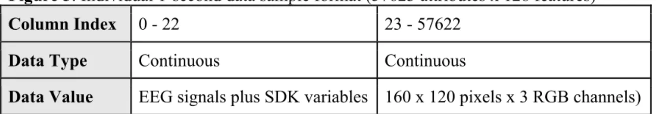
3.4.1 Preprocessed Data Format

In its raw preprocessed form, each second (or sample) of data is stored in an .arff file containing 23 attributes relating to the EEG device (14 sensors and 9 software specific metrics).

The remaining attributes in each row represent the image captured by the video camera at the time of recording. Each file contains 128 rows, where one row stores the data for each EEG device sample iteration. Recall that the EEG device operates at 128 samples per second, whereas the video camera is only able to capture 30 frames per second. The preprocessed data therefore contains video data redundancy.

Figure 5: Individual 1-second data sample format (57623 attributes x 128 features)

Column Index 0 - 22 23 - 57622

Data Type Continuous Continuous

Data Value EEG signals plus SDK variables 160 x 120 pixels x 3 RGB channels)

3.4.2 Processed Data Format

The data was processed in order to isolate the individual EEG signals from the complete EEG data, excluding irrelevant information such as timestamps, gyroscope readings, and sample counters. In order to compress the scale of the video data, PCA was applied to the video data to compress the information for easier computation without sacrificing too much content meaning.

Principal Component Analysis (PCA) is a powerful statistical procedure for both dimensionality reduction and linear decorrelation [2, 4]. Given a sample of non-Gaussian data, Plumbley argued that PCA minimizes the upper bound on the information lost due to

dimensionality reduction [3]. Because of its capacity to minimize dimensionality, redundancy, and information loss, PCA was applied to reduce the video components to 30 dimensions.

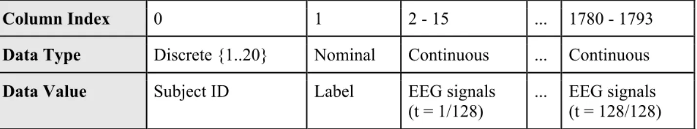
The method produced two master datasets, a control set with only EEG information and a hypothesis set containing both EEG and video data. Each row in the master datasets reflects a full second of chronological data with 128 individual samples.

Figure 6: EEG only master data set format (1794 attributes x variable # rows). In this figure, t represents the number of samples relative to the sample rate per second.

Column Index 0 1 2 - 15 ... 1780 - 1793

Data Type Discrete {1..20} Nominal Continuous ... Continuous

Data Value Subject ID Label EEG signals

(t = 1/128)

... EEG signals (t = 128/128)

Figure 7: EEG and video master data set format (5634 attributes x variable # rows). In this figure, t represents the number of samples relative to the sample rate per second.

Column Index 0 1 2 - 15 16 - 45 ... 5590 - 5603 5604 - 5633 Data Type Discrete {1..20}

Nominal Continuous Continuous ... Continuous Continuous

Data Value

Subject ID

Label EEG signals

(t = 1/128) Video PCA (t =1/128) ... EEG signals (t = 128/128) Video PCA (t = 128/128) 3.5 Algorithms

The Waffles machine learning toolkit was used to implement these experiments. Waffles is an open source collection of machine learning algorithms and tools in C++ [29]. To test the significance of adding video components to the EEG signals, a Waffles implementation of the random forest algorithm was used. Recall the benefits of the RF algorithm: its proven ability to extract features from EEG signals, its capacity for high-dimensional data, and its efficient computational costs. To measure the results of these experiments, cross-validation was used to generate mean-squared error (MSE). Cross-validation not only provides useful metrics for measuring accuracy but also assesses how well the classifying model can generalize to an independent data set [30]. Other algorithms used during these experiments include PCA and significance analysis to determine if the comparison passes the one-tailed p-test with a p-value of 0.05 or less.

4. RESULTS AND ANALYSIS 4.1 Methodology

The primary metric for evaluating the success of the project experiments is predictive accuracy, which is obtained by calculating mean squared error (MSE) during cross validation. Cross validation The MSE statistic was calculated according to the following equation:

!"# =_!! ! !_! −!_! !

!!! , where ! is a vector of ! label predictions, and ! is a vector representing the actual labels. Predictive accuracy (PA) is measured by subtracting the MSE from 1.

4.2 Results

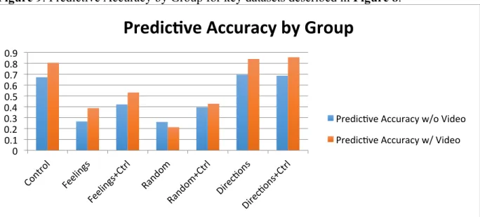
Across the board, the conducted experiments indicated that the addition of video data in conjunction with simultaneous EEG data collection significantly enhanced the predictive accuracy of the classifier. The experiments were conducted for 7 different groupings: 4 groupings for the original Control, Feelings, Random, and Directions groups, and 3 groupings for the hypothesis groups (Feelings, Random, and Directions) plus the Control group. A table of the overall results from each of the label groupings is shown below.

Figure 8: Overall predictive accuracy results for key datasets.

Group PA w/o Video PA w/ Video % Change

Control 0.672209026 0.804750594 0.197173145 Feelings 0.265882353 0.388235294 0.460176991 Feelings+Control 0.421615202 0.531591449 0.26084507 Random 0.261 0.2125 -0.185823755 Random+Control 0.395577396 0.428173628 0.082401656 Directions 0.695029486 0.839595619 0.208 Directions+Control 0.685920578 0.856028881 0.248

The table in Figure 8 describes the predictive accuracies for EEG data alone and EEG data with concurrent video stream data, as well as the percent change between the two

aforementioned categories. For all but one of the groups, the addition of video input improved predictive accuracy by 8% – 46%. This dataset’s p-value of 0.010630619 demonstrates a significant comparison between predictive accuracy with and without video data.

Figure 9: Predictive Accuracy by Group for key datasets described in Figure 8.

Figure 9 above shows an alternate visualization of the results in Figure 8. This graph makes it clear that every hypothesis category containing the control group (Feelings+Ctrl, Random+Ctrl, Directions+Ctrl) performs better than the hypothesis groups alone (Feelings, Random, Directions). This shows that the addition of control data representing common sources of noise improves the PA of the classifying algorithm.

Figure 10: Percent change in PA without video vs. PA with video data as described in Figure 8.

0" 0.1" 0.2" 0.3" 0.4"0.5" 0.6"0.7" 0.8" 0.9"

Predic've)Accuracy)by)Group)

%)Change)

As Figure 10 demonstrates, the Random group was the outlier in this data set, as the addition of video actually hindered the predictive accuracy of the classifier. This result is not unexpected, since the Random group had the largest vocabulary size and the smallest number of samples per word. When the Random dataset is disregarded, the overall p-value comparing the significance of the inclusion or exclusion of video data is 0.0090079216. Even without

discarding the Random group, the dataset’s p-value of 0.010630619 demonstrates significance.

Figure 11: Percentage change for each hypothesis category, divided by subject.

Figure 11 illustrates the percentage change from PA without video to PA with video data for each category containing the control group, divided by subject and including the average of all the subjects. Please note that the categories explored in this graph represent only the

hypothesis groups containing the control group. This graph highlights the variance in the percent change from subject-to-subject. For example, each percentage change for Subject 2 yields a lower PA, indicating that video data does not help the classifier identify patterns in the EEG

1" 2" 3" 4" 5" 6" 7" 8" 9" _{10" 11" 12" 13" 14" 15" 16" 17" 18" 19" 20"} AV G" =0.6" =0.4" =0.2" 0" 0.2" 0.4" 0.6" 0.8" 1" 1.2" 1.4" 1.6" Percen ta ge)Ch an ge) _{Control"%"Change"} Feelings+Ctrl"%"Change" Random+Ctrl"%"Change" Direc3ons+Ctrl"%"Change"

signals collected for Subject 2. By contrast, Subject 6 yields the highest percentage change of all the subjects in every category except one. Therefore, the addition of video data greatly increases the classifier’s ability to extract meaning from Subject 6’s EEG signals. For a more detailed breakdown of the experiment results by subject, please refer to the Data Appendix.

4.3 Analysis

The experimental results confirm the hypothesis that supplementing EEG data with simultaneous video data will allow for a classifying algorithm to more effectively facilitate imagined speech recognition. While there are a few outlier cases, there is a significant correlation between a classifier’s PA without video and PA with video data. Since video data improves the predictive accuracy of the classifying algorithm, the classifier must have learned to correlate visual cues to important features or sources of noisiness in the EEG data.

The experiments show that the addition of video data improved the classifier’s PA, particularly when analyzing the Directions, Directions+Ctrl, Feelings, and Feelings+Ctrl groups, as shown by Figure 10. One possible reason for this higher percentage change may be a

symptom of how human brains process feelings and movements. Other researchers have observed that when a user is thinking of ideas that evoke a strong physical response, like movements or feelings, the patterns of change in these EEG signals is dramatic enough for classifiers to identify with greater accuracy [14, 16]. Conversely, the classifier was not able to demonstrate predictive accuracy as well when presented with the Random and Random+Ctrl group. This result is not unexpected because the Random group of labels contains the greatest number of labels, the least number of samples per label, and is not known to produce strong reactions in EEG signals.

Referring back to Figure 8, when the classifier tested with the Control group alone, the percentage change in PA was not as dramatic as it was for the Feelings+Ctrl or Directions+Ctrl groups. This is an unexpected result, since both the Feelings+Ctrl and Directions+Ctrl groups had more labels and a lesser number of samples per word. This find suggests that although the classifier is using the extra information about the subject’s environment to successfully separate the signal from the noise in EEG features, the classifier is not as well suited to delineate between different types of noise in EEG signals. Despite the classifier’s ability to recognize noise in EEG data, the results from this project may indicate that classifiers are not as effective at delineating between sources of noise. Further investigation is required to confirm this speculation.

5. CONCLUSIONS 5.1 Summary

The results from this project suggest confirmation of the hypothesis that adding high-dimensional data relating to a subject’s environment, such as video data, to complement EEG readings enhances a classifier’s ability to facilitate imagined speech recognition. Although the relative effectiveness of this method is highly dependent on the individual subject, this project showed that the addition of video data in conjunction with simultaneous EEG data collection enhances the predictive accuracy of the classifier.

Possibilities for future research include incorporating additional information about a subject’s environment in a dataset. For example, higher resolution video with a higher frames-per-second rate may be able to provide a classifier with more accurate data about the subject’s environment. Another additional data source to experiment with is concurrent audio data. It follows that audio data would help to de-noise a dataset and prevent a subject’s EEG response to audible stimulus from skewing the classifier’s feature extraction capabilities. It would also be useful to test the robustness of this approach by experimenting with dynamic predictions with randomly ordered words immediately following the data acquisition process.

5.2 Potential Impact

Advancements in imagined speech recognition have the potential to make an impact in a variety of domains, such as wheelchair or prosthesis control for paraplegics or disabled persons, or communication with persons suffering from locked-in syndrome, a condition where patients are conscious but unable to produce speech or movement [12]. Fluid BCIs enabled by imagined speech recognition would improve the notoriously cumbersome interface between humans and computing devices, and offer new paths for neurological research [11].

DATA APPENDIX

Breakdown of Percentage Change by Subject and Grouping

Subje ct Control % Change Feelings+Ctrl % Change Random+Ctrl % Change Directions+Ctrl % Change 1 0.275362319 0.224719101 0.206521739 0.107142857 2 -0.09375 -0.387931034 -0.209090909 -0.248730964 3 0.442622951 0.516129032 0.829268293 1.077419355 4 0.053763441 0.082089552 0.027027027 0.073170732 5 0.342857143 0.31092437 0.295238095 -0.052287582 6 0.551724138 0.708860759 0.753246753 1.381355932 7 0.265822785 0.137614679 0.124087591 0.111510791 8 0.275362319 0.201923077 -0.050955414 0.144366197 9 0.380952381 0.666666667 0.148148148 0.386934673 10 0.116883117 0.204545455 -0.013513514 0.025641026 11 0.24691358 -0.03539823 0.02238806 0.324444444 12 0.482758621 0.480519481 0.024793388 0.213178295 13 0.222222222 0.269662921 0.071428571 0.169421488 14 0.166666667 0.058252427 -0.299270073 0 15 0 0.258426966 -0.068965517 0.153846154 16 0.306666667 0.051546392 -0.2 -0.051948052 17 0.131578947 0.523255814 0.040322581 0.031468531 18 0.24 0.082474227 0.008264463 -0.019736842 19 0 0.227272727 0.056451613 0.264925373 20 0.323529412 0.46835443 0.115789474 0.035856574 AVG 0.236596836 0.252495441 0.094059018 0.206398949 1" 2" 3" 4" 5" 6" 7" 8" 9" _{10" 11" 12" 13" 14" 15" 16" 17" 18" 19" 20"} AV G" =0.6" =0.4" =0.2" 0" 0.2" 0.4" 0.6" 0.8" 1" 1.2" 1.4" 1.6" Percen ta ge)Ch an ge) _{Control"%"Change"} Feelings+Ctrl"%"Change" Random+Ctrl"%"Change" Direc3ons+Ctrl"%"Change"

Control Group by Subject

Subject Predictive Accuracy w/o Video Predictive Accuracy w/ Video % Improvement

1 0.657142857 0.838095238 0.275362319 2 0.60952381 0.552380952 -0.09375 3 0.580952381 0.838095238 0.442622951 4 0.885714286 0.933333333 0.053763441 5 0.666666667 0.895238095 0.342857143 6 0.552380952 0.857142857 0.551724138 7 0.752380952 0.952380952 0.265822785 8 0.657142857 0.838095238 0.275362319 9 0.6 0.828571429 0.380952381 10 0.733333333 0.819047619 0.116883117 11 0.736363636 0.918181818 0.24691358 12 0.552380952 0.819047619 0.482758621 13 0.771428571 0.942857143 0.222222222 14 0.8 0.933333333 0.166666667 15 0.79047619 0.79047619 0 16 0.714285714 0.933333333 0.306666667 17 0.723809524 0.819047619 0.131578947 18 0.714285714 0.885714286 0.24 19 0.690909091 0.690909091 0 20 0.68 0.9 0.323529412 AVG % IMPROVEMENT 0.236596836 P-VALUE 7.52E-05

Feelings+Ctrl Group by Subject 0" 0.1" 0.2" 0.3" 0.4" 0.5" 0.6" 0.7" 0.8" 0.9" 1" 1" 2" 3" 4" 5" 6" 7" 8" 9" 10"11"12"13"14"15"16"17"18"19"20"

Control)Group)Results)by)Subject)

Subject Predictive Accuracy w/o Video Predictive Accuracy w/ Video % Improvement 1 0.423809524 0.519047619 0.224719101 2 0.552380952 0.338095238 -0.387931034 3 0.43255814 0.655813953 0.516129032 4 0.638095238 0.69047619 0.082089552 5 0.566666667 0.742857143 0.31092437 6 0.376190476 0.642857143 0.708860759 7 0.519047619 0.59047619 0.137614679 8 0.495238095 0.595238095 0.201923077 9 0.357142857 0.595238095 0.666666667 10 0.419047619 0.504761905 0.204545455 11 0.525581395 0.506976744 -0.03539823 12 0.366666667 0.542857143 0.480519481 13 0.423809524 0.538095238 0.269662921 14 0.49047619 0.519047619 0.058252427 15 0.423809524 0.533333333 0.258426966 16 0.461904762 0.485714286 0.051546392 17 0.40952381 0.623809524 0.523255814 18 0.461904762 0.5 0.082474227 19 0.409302326 0.502325581 0.227272727 20 0.385365854 0.565853659 0.46835443 AVG % IMPROVEMENT 0.252495441 P-VALUE 0.00027211 0" 0.1" 0.2" 0.3" 0.4" 0.5" 0.6" 0.7" 0.8" 1" 2" 3" 4" 5" 6" 7" 8" 9" 10" 11" 12" 13" 14" 15" 16" 17" 18" 19" 20"

Feelings+Ctrl)Group)Results)by)Subject)

Random+Ctrl Group by Subject

Subject Predictive Accuracy w/o Video Predictive Accuracy w/ Video % Improvement

1 0.296774194 0.358064516 0.206521739 2 0.360655738 0.285245902 -0.209090909 3 0.268852459 0.491803279 0.829268293 4 0.485245902 0.498360656 0.027027027 5 0.344262295 0.445901639 0.295238095 6 0.252459016 0.442622951 0.753246753 7 0.449180328 0.504918033 0.124087591 8 0.514754098 0.48852459 -0.050955414 9 0.354098361 0.406557377 0.148148148 10 0.485245902 0.478688525 -0.013513514 11 0.446666667 0.456666667 0.02238806 12 0.396721311 0.406557377 0.024793388 13 0.413114754 0.442622951 0.071428571 14 0.449180328 0.314754098 -0.299270073 15 0.380327869 0.354098361 -0.068965517 16 0.459016393 0.367213115 -0.2 17 0.4 0.416129032 0.040322581 18 0.396721311 0.4 0.008264463 19 0.4 0.422580645 0.056451613 20 0.316666667 0.353333333 0.115789474 AVG % IMPROVEMENT 0.094059018 P-VALUE 0.04179601 0" 0.1" 0.2" 0.3" 0.4" 0.5" 0.6" 1" 2" 3" 4" 5" 6" 7" 8" 9" 10"11"12"13"14"15"16"17"18"19"20"

Random+Ctrl)Group)Results)by)Subject)

Directions+Ctrl Group by Subject

Subject Predictive Accuracy w/o Video Predictive Accuracy w/ Video % Improvement

1 0.8 0.885714286 0.107142857 2 0.656666667 0.493333333 -0.248730964 3 0.455882353 0.947058824 1.077419355 4 0.831884058 0.892753623 0.073170732 5 0.874285714 0.828571429 -0.052287582 6 0.337142857 0.802857143 1.381355932 7 0.794285714 0.882857143 0.111510791 8 0.811428571 0.928571429 0.144366197 9 0.568571429 0.788571429 0.386934673 10 0.891428571 0.914285714 0.025641026 11 0.652173913 0.863768116 0.324444444 12 0.747826087 0.907246377 0.213178295 13 0.691428571 0.808571429 0.169421488 14 0.862857143 0.862857143 0 15 0.742857143 0.857142857 0.153846154 16 0.88 0.834285714 -0.051948052 17 0.817142857 0.842857143 0.031468531 18 0.868571429 0.851428571 -0.019736842 19 0.765714286 0.968571429 0.264925373 20 0.717142857 0.742857143 0.035856574 AVG % IMPROVEMENT 0.206398949 P-VALUE 0.001372801 0" 0.2" 0.4" 0.6" 0.8" 1" 1.2" 1" 2" 3" 4" 5" 6" 7" 8" 9" 10"11"12"13"14"15"16"17"18"19"20"

Direc'ons+Ctrl)Group)Results)by)Subject)

REFERENCES

[1] K. Brigham and B. V. K. V. Kumar, "Imagined Speech Classification with EEG Signals for Silent Communication: A Preliminary Investigation into Synthetic Telepathy," Bioinformatics

and Biomedical Engineering (iCBBE), 2010 4th International Conference on, Chengdu, 2010,

pp. 1-4. doi: 10.1109/ICBBE.2010.5515807

URL: http://ieeexplore.ieee.org/stamp/stamp.jsp?tp=&arnumber=5515807&isnumber=5514659 [2] Bernard C. Geiger and Gernot Kubin, “Relative Information Loss in the PCA,” IEEE

Information Theory Workshop, 2012, pp. 562 - 566. doi: 10.1109/ITW.2012.6404738

URL: http://arxiv.org/abs/1204.0429v2

[3] M. Plumbley, “Information theory and unsupervised neural networks,” Cambridge University Engineering Department, Tech. Rep. CUED/F-INFENG/TR. 78, 1991.

[4] G. Deco and D. Obradovic, An Information-Theoretic Approach to Neural Computing. New York, NY: Springer, 1996.

[5] Kevin Whittingstall, Nikos K. Logothetis, Frequency-Band Coupling in Surface EEG Reflects Spiking Activity in Monkey Visual Cortex, Neuron, Volume 64, Issue 2, 29 October 2009, Pages 281-289, ISSN 0896-6273, http://dx.doi.org/10.1016/j.neuron.2009.08.016. (http://www.sciencedirect.com/science/article/pii/S089662730900628X)

[6] L. Hausfeld, F. De Martino, M. Bonte, and E. Formisano, “Pattern analysis of eeg responses to speech and voice: Influence of feature grouping,” NeuroImage, vol. 59, no. 4, pp. 3641–3651, 2012.

[7] A. Martins and P. Rincon, “Paraplegic in robotic suit kicks off world cup,” June 2014. [Online]. Available: http://www.bbc.com/news/science-environment-27812218

[8] N. Birbaumer, T. Hinterberger, A. Kubler, and N. Neumann, “The thought-translation device (ttd): neurobehavioral mechanisms and clinical outcome,” Neural Systems and Rehabilitation

Engineering, IEEE Transactions on, vol. 11, no. 2, pp. 120–123, 2003.

[9] A. Chan, C. E. Early, S. Subedi, Yuezhe Li and H. Lin, "Systematic analysis of machine learning algorithms on EEG data for brain state intelligence," Bioinformatics and Biomedicine

(BIBM), 2015 IEEE International Conference on, Washington, DC, 2015, pp. 793-799.

doi: 10.1109/BIBM.2015.7359788 URL:

http://0-ieeexplore.ieee.org.library.uark.edu/stamp/stamp.jsp?tp=&arnumber=7359788&isnumber=7359 638

[10] Dr. Gashler’s unpublished book manuscript: http://uaf46365.ddns.uark.edu/lab/ml.pdf [11] My SURF Grant proposal

[12] [5] Laureys, Steven, et al. "The locked-in syndrome: what is it like to be conscious but paralyzed and voiceless?." Progress in brain research 150 (2005): 495-611.

[13] F. Lotte, M. Congedo, A. Lecuyer, F. Lamarche, B. Arnaldi ´ et al., “A review of classification algorithms for eeg-based brain–computer interfaces,” Journal of neural engineering, vol. 4, 2007.

[14] L. Hausfeld, F. De Martino, M. Bonte, and E. Formisano, “Pattern analysis of eeg responses to speech and voice: Influence of feature grouping,” NeuroImage, vol. 59, no. 4, pp. 3641–3651, 2012.

[15] Wester, M., and T. Schultz. "Unspoken speech-speech recognition based on

electroencephalography." Master's thesis, Universität Karlsruhe (TH), Karlsruhe, Germany (2006).

[16] Brian Murphy, Marco Baroni, and Massimo Poesio. 2009. EEG responds to conceptual stimuli and corpus semantics. In Proceedings of the 2009 Conference on Empirical Methods in

Natural Language Processing: Volume 2 - Volume 2 (EMNLP '09), Vol. 2. Association for

Computational Linguistics, Stroudsburg, PA, USA, 619-627.

[17] C. A. Joyce, I. F. Gorodnitsky, and M. Kutas, “Automatic removal of eye movement and blink artifacts from eeg data using blind component separation,” Psychophysiology, vol.41, no.2, pp.313–325, 2004.

[18] A. Subasi and E. Ercelebi, “Classification of eeg signals using neural network and logistic regression,” Computer Methods and Programs in Biomedicine, vol. 78, no. 2, pp. 87–99, 2005. [19] Paul L. Nunez, Electroencephalography (EEG), In Encyclopedia of the Human Brain, edited by V.S. Ramachandran,, Academic Press, New York, 2002, Pages 169-179, ISBN

9780122272103, http://0-dx.doi.org.library.uark.edu/10.1016/B0-12-227210-2/00128-X. [20] S. Zhao and F. Rudzicz, "Classifying phonological categories in imagined and articulated speech," 2015 IEEE International Conference on Acoustics, Speech and Signal Processing

(ICASSP), South Brisbane, QLD, 2015, pp. 992-996.

doi: 10.1109/ICASSP.2015.7178118

[21] S. Iqbal, Y. U. Khan and O. Farooq, "EEG based classification of imagined vowel sounds," Computing for Sustainable Global Development (INDIACom), 2015 2nd International

[22] D. Wulsin, J. Gupta, R. Mani, J. Blanco, and B. Litt, “Modeling electroencephalography waveforms with semi-supervised deep belief nets: fast classification and anomaly measurement,”

Journal of neural engineering, vol. 8, no. 3, p. 036015, 2011

[23] J. Turner, A. Page, T. Mohsenin, and T. Oates, “Deep belief networks used on high

resolution multichannel electroencephalography data for seizure detection,” in 2014 AAAI Spring

Symposium Series, 2014.

[24] ] C. W. Anderson, S. V. Devulapalli, and E. A. Stolz, “Determining mental state from eeg signals using parallel implementations of neural networks,” Scientific programming, vol.4, no.3, pp.171–183, 1995.

[25] Patrick Suppes, Zhong-Lin Lu, and Bing Han, "Brain wave recognition of words,"

Proceedings of the National Academy of Sciences, vol. 94, no. 26, pp. 14965- 14969,1997.

[26] Anne Porbadnigk, Marek Wester, Jan Calliess, and Tanja Schultz, "EEG-based speech recognition - impact of temporal effects.," in BIOSIGNALS, Pedro Encarnao and Antnio Veloso, Eds. 2009, pp. 376-381, INSTICC Press.

[26] A. Vuckovic, V. Radivojevic, A. C. Chen, and D. Popovic, “Automatic recognition of alertness and drowsiness from eeg by an artificial neural network,” Medical Engineering &

Physics, vol. 24, no. 5, pp. 349–360, 2002.

[27] D. Gallez and A. Babloyantz, “Predictability of human eeg: a dynamical approach,”

Biological Cybernetics, vol. 64, no. 5, pp. 381–391, 1991.

[28] B. Obermaier, C. Guger, C. Neuper, and G. Pfurtscheller, “Hidden markov models for online classification of single trial eeg data,” Pattern recognition letters, vol. 22, no. 12, pp. 1299–1309, 2001.

[29] M. S. Gashler, “Waffles: A machine learning toolkit,” Journal of Machine Learning

Research, vol. MLOSS 12, pp. 2383–2387, July 2011. [Online]. Available:

http://www.jmlr.org/papers/volume12/ gashler11a/gashler11a.pdf

[30] Kohavi, Ron. "A study of cross-validation and bootstrap for accuracy estimation and model selection." Ijcai. Vol. 14. No. 2. 1995.