Louisiana State University
LSU Digital Commons
LSU Doctoral Dissertations Graduate School
2012
Aggregate analyst forecast errors, price delay, and
business cycle
Ping-Wen Sun
Louisiana State University and Agricultural and Mechanical College, [email protected]
Follow this and additional works at:https://digitalcommons.lsu.edu/gradschool_dissertations
Part of theFinance and Financial Management Commons
This Dissertation is brought to you for free and open access by the Graduate School at LSU Digital Commons. It has been accepted for inclusion in LSU Doctoral Dissertations by an authorized graduate school editor of LSU Digital Commons. For more information, please [email protected]. Recommended Citation
Sun, Ping-Wen, "Aggregate analyst forecast errors, price delay, and business cycle" (2012).LSU Doctoral Dissertations. 3427.
AGGREGATE ANALYST FORECAST ERRORS, PRICE DELAY, AND BUSINESS CYCLE
A Dissertation
Submitted to the Graduate Faculty of the Louisiana State University and Agriculture and Mechanical College
in partial fulfillment of the requirements for the degree of
Doctor of Philosophy
In
The Interdepartmental Program in Business Administration (Finance)
by Ping-Wen Sun
B.S., National Taiwan University, 1997 M.S., National Taiwan University, 1999 M.B.A., Binghamton University, 2006
ii
ACKNOWLEDGEMENTS
I want to thank Professor Jimmy E. Hilliard for giving me the chance to join the finance
PhD program at LSU and the opportunity of working with Professor Ji-Chai Lin. I enjoy every
moment whenever I discuss research ideas with Professor Lin. Besides in the professional area,
Professor Lin also helps me understand myself in many aspects in life. I admire his wisdom and
regard him as my lifelong role model to follow. Professor William R. Lane and Professor V.
Carlos Slawson at LSU Department of Finance not only give me the chance to pursue a higher
education in the United States, but they also give me the opportunity to serve students. Through
past several semesters, I have developed solid teaching skills and strengthened my knowledge in
the finance field. I will abide by the "lifetime students" philosophy of the finance PhD program
after my graduation and work hard to transfer this important and useful thinking to every friend
and student in my life.
Professor Gary C. Sanger teaches me the foundations of financial economics. Professor
Wei-Ling Song teaches me empirical research topics related to banking and helps me develop
my critical thinking about every paper. Both of them provide valuable services to be my
committee members and help me a lot during my job search process. Professor Fan Chen and
Li-Wen Chen teach me how to deal with obstacles in life and kindly provide me with the physical
and mental shelter whenever I need help. Professor Faik A. Koray teaches me the fundamental
macroeconomics and also helps me as my committee member. Professor Kenneth J Reichelt
kindly improves my dissertation from the accounting perspective and also serves as my
iii
During my six-year stay at LSU, I make many good friends at LSU. I want to give my
thanks to all of them and hope them to enjoy a better life after they finish their studies here.
Many old friends also provide valuable support and encouragement whenever I need them.
Finally, I want to give my special thanks to my parents. They selflessly and unconditionally care
about me and provide the financial support whenever I need it. Without all the help I have
received in my life, there is no possibility that I could have some achievements if there is any.
Although I cannot stay at LSU forever, I will carry everything I've learned here and seek every
iv TABLES OF CONTENTS ACKONWLEDGEMENTS...ii LIST OF TABLES...vi LIST OF FIGURES...vii ABSTRACT...viii CHAPTER 1: INTRODUCTION...1
CHAPTER 2: STOCK MARKET LIQUIDITY, AGGREGATE ANALYST FORECAST ERRORS, AND THE ECONOMY...3
2.1 Introduction...3
2.2 Literature Review and Hypothesis...7
2.2.1 Analysts and Information Production...7
2.2.2 The Flight-to-quality Behavior of Investors...9
2.2.3 Hypothesis...11
2.3 Data...11
2.3.1 Stock Market Liquidity...11
2.3.2 Analyst Forecast Errors...12
2.3.3 Economy Data...14
2.3.4 Summary Statistics of the Variables...16
2.4 Regression Results...18
2.4.1 Predicting Aggregate Analyst Forecast Errors...22
2.4.2 The Source of the Economic Forecastability of Stock Market Liquidity...23
2.5 Conclusion...27
CHAPTER 3: STOCK PRICE DELAY AND BUSINESS CYCLE...33
3.1 Introduction...33
3.2 Literature Review...39
3.2.1 Market Frictions Hypothesis...39
3.2.2 Information Production Hypothesis...41
3.2.3 Flight-to-quality Hypothesis...42
3.3 Data...44
3.3.1 Price Delay Measure...44
3.3.2 GDP Growth...46
3.3.3 Market Frictions Variable...46
3.3.4 Information Production Variables...47
3.3.5 Flight-to-quality Variables...48
3.4 Results...49
3.4.1 Summary Statistics of Variables...49
v
3.5 Conclusion...61
CHAPTER 4: CONCLUSION...66
REFERENCES...67
vi
LIST OF TABLES
2.1 Summary Statistics of the Relevant Variables...19
2.2 Correlation Matrix...20
2.3 Predicting Aggregate Analyst Forecast Errors...24
2.4 Aggregate Analyst Forecast Errors and Stock Market Liquidity Changes...25
2.5 GDP Growth Rate, Stock Market Liquidity Change, and Predicted Aggregate Analyst Forecast Error...29
2.6 Stock Market Liquidity and the Components of GDP Growth...30
3.1 Sample Characteristics...53
3.2 Correlation Matrix...54
3.3 Aggregate Price Delay Change and Real GDP Growth...58
3.4 Aggregate Price Delay and Market Frictions...59
3.5 Aggregate Price Delay and Information Production...59
vii
LIST OF FIGURES
2.1 Aggregate Standardized Analyst Forecast Errors (AAFE) and Their Time Trend...15
2.2 Detrended Aggregate Analyst Forecast Errors (detrended_AAFE) and GDP
Growth...21
3.1 Aggregate Stock Price Delay and Real GDP Growth...50
3.2 Lagged Aggregate Stock Price Delay Change and Real GDP Growth...51
3.3 Aggregate Stock Price Delay in the Quarters around the Past 11 Recession
Starting Quarter...51
3.4 Aggregate Stock Price Delay in the Quarters around the Past 11 Recession
viii ABSTRACT
This dissertation consists of two essays. The first essay, “Stock market liquidity,
aggregate analyst forecast errors, and the economy,” is motivated by Næs, Skjeltorp, and
Ødegaard (2011), who suggest that stock market liquidity is a good leading indicator of the
economy. To further understand the mechanism in the economic forecastability of stock market
liquidity, we hypothesize that analyst earnings forecast errors have a systematic component,
which is predictable and related to changes in the economy, and that smart investors exploit
analyst forecast errors, which leads to the economic forecastability of stock market liquidity.
Consistent with our hypothesis, we find that there is a strong correlation between detrended
aggregate analyst forecast errors and concurrent GDP growth and that a large part of the forecast
errors can be predicted using lagged macro variables. Once we control for the predictable
forecast errors, the economic forecastability of stock market liquidity disappears. Thus, our study
reveals that aggregate analyst forecast errors are very informative about business cycle and
contain all the relevant information for stock market liquidity as a leading economic indicator.
The second essay, “Stock price delay and business cycle,” is motivated by Hou and
Moskowitz (2005), who use common stock price delay in reflecting market-wide information to
measure market frictions each individual firm faces. To better understand how the price
formation process is affected by business cycle, we examine the relation between the aggregate
stock price delay and changes in the economy. Surprisingly, while the stock market liquidity
declines and market frictions increase before economic downturns, we find that the aggregate
price delay decreases before recessions; and it increases before economic expansions when the
ix
and aggregate analyst coverage as proxies for information production cannot account for the
behavior of aggregate price delay. Instead, we find that the flight-to-quality behavior of investors
1
CHAPTER 1: INTRODUCTION
This dissertation consists of two essays. The first one, “stock market liquidity, aggregate analyst forecast errors, and the economy,” studies the role played by aggregate analyst forecast errors in the economic predictability of stock market liquidity, and the second essay, “stock price
delay and business cycle,” examines what factors may affect aggregate stock price delay during a business cycle. The common theme of my two essays is how the economy and the stock market
are interrelated, particularly on how market frictions anticipate and react to changes in economic
conditions.
Næs, Skjeltorp, and Ødegaard (2011) document stock market liquidity has a predicting
power on future economy. My first essay extends their finding and addresses the following
research questions. Since trading in the stock market affects stock market liquidity, could trading
from more informed investors provide an explanation for the predictability of stock market
liquidity on future economy? In addition, because analysts' earnings forecasts of firms influence
investors' expectation about future economy, could aggregate analyst forecast errors play a role
to facilitate those informed investors to utilize their information advantage over other investors?
We find that aggregate analyst forecast errors are predictable and that stock market liquidity
loses its explanation power on future economy once we control aggregate analyst forecast errors.
Our findings suggest that informed investors foresee changes of economy unexpected by analysts
and aggregate analyst forecast errors help informed investors' trading on their private information.
Hou and Moskowitz (2005) document that stocks with a delay to reflect public market
information possess a price delay premium cross-sectionally. In a time series fashion, my second
essay studies whether stocks reflect public market information at different speeds during a
2
starts and tends to increase after a recession ends. Even though Hameed, Kang, Viswanathan
(2010) document stock market liquidity worsens when stock market declines, the trading
difficulty does not seem to delay public market information impounded into stocks. In addition,
although Brockman, Liebenberg, and Schutte (2010) document information production activities
are pro-cyclical, lower information production activities also fail to account for the pro-cyclical
behavior of aggregate stock price delay. We find that the flight-to-quality behavior of investors
mentioned in McQueen, Pinegar, and Thorley (1996) and Næs, Skjeltorp, and Ødegaard (2011)
are most responsible for the pro-cyclical aggregate stock price delay behavior. Our findings help
our understanding of stock price formation process during a business cycle and suggest
aggregate stock price delay could be a state variable.
This dissertation contributes to our understanding of the systematic component of
financial analysts earnings forecast errors, stock price delay changes in a business cycle, and
flight-to-quality behavior of investors. First of all, aggregate analyst forecast errors highly
correlate with concurrent GDP growth and could be predicted by past macro variables such as
stock market excess return, stock market volatility, term spread, and default spread. Our findings
suggest aggregate analyst forecast errors also help informed trading and provide an explanation
of the predictability of stock market liquidity on the economy. Second, aggregate stock price
delay exhibits a pro-cyclical pattern. The information quality of the stock market seems better
when the economy is bad and when the uncertainty of investors is high. Finally, aggregate
analyst forecast errors facilitate to-quality behavior of smart investors. In addition,
flight-to-quality behavior of investors is most responsible for the pro-cyclical behavior of aggregate
stock price delay. Those findings further help us understand the interaction between the stock
3
CHAPTER 2: STOCK MARKET LIQUIDITY, AGGREGATE ANALYST FORECAST ERRORS, AND THE ECONOMY
2.1 Introduction
Stock market liquidity usually starts to fall before recessions. According to Næs,
Skjeltorp, and Ødegaard (2011), this phenomenon is closely related to the “flight-to-quality”
behavior of investors.1 Their finding suggests that a group of smart investors could foresee the
future economy conditions which could not be predicted by other investors who buy shares sold
by those smart investors. When anticipating economic downturns, in order to protect their wealth,
smart investors adjust their portfolio compositions from riskier and less liquid stocks to stocks
with higher liquidity and lower risk, Treasury securities, or even just cash. Their sells tend to
lead stock market liquidity to decrease. As a result, we often observe declines in overall stock
market liquidity level before recessions start. Thus, Næs et al. (2011) suggest that stock market
liquidity is a good leading indicator of the economy. In this paper, we extend their study to
provide a better understanding of the channel through which stock market liquidity is a good
economic predictor. Our main finding is that smart investors’ economic forecastability is largely built on foreseeing systematic analyst forecast errors, which are predictable and vary with
business cycle.
Financial analysts spend their efforts on gathering, studying, and analyzing available
information on individual companies and then forecast their earnings. Fried and Givoly (1982)
document that financial analyst forecasts provide a better surrogate for market expectations than
those generated by time-series models because analysts tend to use a broader information set and
1
According to Næs, Skjeltorp, and Ødegaard (2011), the term “flight-to-quality” refers to a situation where market participants suddenly shift their portfolios toward securities with less risk.
4
more timely information.2 Recently, Howe, Unlu, and Yan (2009) further show that, in addition
to firm-specific information, analyst recommendations are also partly based on market-level and
industry-level information. They find that aggregation of analysts’ stock recommendations
cancels out the idiosyncratic components and that the aggregate analyst recommendations
corrrespond to systematic factors. They also find that changes in the aggregate analyst
recommendations can predict future stock market returns. Their finding suggests that aggregate
analyst recommendations are informative and useful to stock market investors.
However, facing economic uncertainty and firm-specific risk factors, analysts are bound
to produce forecast errors on individual firms’ earnings. Furthermore, financial analysts may also provide biased reports. For example, Dreman and Berry (1995) find that analysts tend to
overestimate earnings, on average, by a significant amount. Similarly, Easterwood and Nutt
(1999) find that analysts underreact to negative information, but overreact to positive
information, which implies that analysts exhibit systematic optimism in response to information.
To explain the optimism behavior, Hong and Kubik (2003) show that controlling for accuracy,
analysts who are optimistic relative to the consensus are more likely to experience favorable job
separations. Thus, in addition to economic uncertainty, analysts’ behavioral bias could add to
their forecast errors.
Following the logic of Howe, Unlu, and Yan (2009), we aggregate individual firms’
analyst earnings forecast errors to cancel out their idiosyncratic components in the forecast errors,
and to isolate their systematic component, which would largely reflect changes in the economy
unforeseen by analysts and their systematic behavioral biases. In particular, if analysts do not
2 See also Givoly and Lakonishok (1979), who document that information on revisions in analysts’ forecasts of earnings is valuable to investors. More recently, Chen and Zhao (2010) show that using direct cash flow (analyst earnings) forecasts, there is a significant component of cash flow news in stock returns.
5
fully anticipate when economic downturns and expansions would occur, their earnings forecasts
are likely to be too optimistic before recessions and too pessimistic before expansions. This
suggests that aggregate analyst earnings forecast errors and changes in the economy are likely to
be correlated.
Would smart investors foresee and exploit systematic analyst forecast errors? If they do,
then systematic analyst forecast errors could be a major culprit in facilitating the
“flight-to-quality” behavior in which smart investors sell risky securities and other (less informed) investors are willing to buy them before economic downturns. Thus, we believe the question is
important and could lead us to better understand the mechanism in the economic forecastability
of stock market liquidity.
Specifically, we hypothesize that analyst earnings forecast errors have a systematic
component, which is predictable and related to changes in the economy, and that smart investors
exploit analyst forecast errors, which leads to the economic forecastability of stock market
liquidity. Our hypothesis is built on the following assumptions. First, smart investors can foresee
analyst earnings forecast errors and sell risky securities when analysts are collectively too
optimistic, and buy risky securities when they are collectively too pessimistic. Second, analysts
tend to be too optimistic (pessimistic) before economic downturns (expansions) occur. Third,
smart investors’ sells (buys) can trigger other market participants to sell (buy) as they learn more about market conditions and lead to decreases (increases) in stock market liquidity.
Thus, our hypothesis suggests that decreases in stock market liquidity would precede
negative aggregate analyst earnings forecast errors (i.e., actual earnings are collectively lower
than analyst forecasts), which tend to take place in economic downturns. Conversely, increases
6
actual earnings are collectively higher than analyst forecasts), which tend to arise during
economic expansions. In other words, our hypothesis suggests that the economic forecastability
of stock market liquidity is through systematic analyst forecast errors.
We test our hypothesis using quarterly real GDP growth to represent the change in
economy in each quarter and our sample period is from 1987Q1 to 2010Q4. Consistent with our
hypothesis, we find a strong correlation between detrended aggregate analyst forecast errors and
concurrent real GDP growth. Furthermore, detrended aggregate analyst forecast errors are
negatively correlated to lagged stock market volatility, and positively correlated to lagged term
spread and lagged market excess returns. Using the lagged macro variables, about one third of
the variation in detrended aggregate analyst forecast errors can be predicted.
The predicted forecast errors have a strong relation with stock market liquidity, while the
part of the forecast errors not predicted by the macro variables has a very weak relation with
stock market liquidity. Interestingly, the economic forecastability of stock market liquidity, as
documented by Næs, Skjeltorp, and Ødegaard (2011), disappear once we control for the
predicted forecast errors. To further illustrate, we decompose real GDP growth into two parts,
one related and the other unrelated to aggregate analyst earnings forecast errors, and find that
while the part of real GDP growth related to aggregate analyst forecast errors can be significantly
explained by the previous quarter’s stock market liquidity change, the part unrelated to the aggregate analyst forecast errors has virtually no relation with the previous quarter’s stock market liquidity change.
In sum, the evidence implies that stock market liquidity as an economic leading indicator
is built on systematic analyst forecast errors. While analysts provide useful information to market
7
capturing smart investors’ collective behavior on systematic analyst forecast errors, becomes informative on changes in the economy.
The rest of the paper is organized as follows. In the next section, we review the literature
on analyst earnings forecasts and on business cycle, and then discuss our hypothesis. Section 1.3
describes the data and the variables used in our study. Section 1.4 reports empirical results, and
sectional 1.5 contains our concluding remarks.
2.2 Literature Review and Hypothesis
This study links two strands of the finance and accounting literature. The first one is
analysts’ information production, and the second strand is the flight-to-quality behavior of investors. We first review each strand of the literature relevant to our study, after which we form
our hypothesis.
2.2.1 Analysts and Information Production
Are financial analysts’ earnings forecasts informative? Givoly and Lakonishok (1979) study the information content of revisions in analyst earnings forecasts by analyzing the relation
between the direction of revisions and stock price behavior. They find that stocks have
significant abnormal returns during the two months following the revision month, suggesting that
analyst earnings forecasts provide useful information to investors and that the information
diffuses over time. Fried and Givoly (1982) further compare analyst earnings forecasts to
predictions generated by time-series models commonly used in research, and show that analyst
forecasts provide a better surrogate for market expectations than forecasts generated by
time-series models. They argue that the advantage of financial analysts’ forecasts comes from two factors: one is the broadness of the information set (firm-specific, industry, and market) available
8
to them and the other is their timing advantage, in that financial analysts employ information that
becomes available after the last accounting reports.
However, numerous studies document biases in analyst forecasts. For example, Dreman
and Berry (1995) examine the quality of analyst earnings forecasts from 1974 through the first
quarter of 1991. They find that analysts’ forecast errors are larger than one might expect; that
these errors are increasing over time; and that analysts are optimistic on the average. Easterwood
and Nutt (1999) show that analysts underreact to negative information but overreact to positive
information and conclude that analysts exhibit systematic optimism in response to information.
Francis and Philbrick (1993) argue that optimistic forecasts allow analysts to maintain close
relationships with company managers, while Clayman and Schwartz (1994) attribute the
optimism to the tendency of analysts to “fall in love” with the stocks they cover. Lim (2001)
suggest that because financial analysts trade off bias to improve management access and forecast
accuracy, statistically optimal forecasts, in the sense of minimum expected squared error, may be
positively and predictably biased. Hong and Kubik (2003) further explain that biased earnings
forecasts may come from analysts’ career concerns. They show that although analysts who produce relatively accurate forecasters are more likely to experience favorable career outcomes,
such as moving up to a high-status brokerage house, after controlling for accuracy, analysts who
are optimistic relative to the consensus are more likely to experience favorable job separations.
Thus, analysts have incentives to provide optimistic reports.
Furthermore, Ljungqvist et al. (2009) demonstrate that analyst optimism increases
chances of analysts’ banks to win co-management appointments, which increases the likelihood of winning underwriting businesses in the future. Malmendier and Shanthikumar (2007) show
9
tend to follow analysts’ buy, hold and sell recommendations literally. Also, Kolasinski and
Kothari (2008) find that target and acquirer analysts use earnings forecasts and recommendations
to increase the odds of approving the deal by shareholders.
Nevertheless, Kadan et al. (2009) document that following the Global Analyst Research
Settlement,3optimistic recommendations have become less frequent and more informative,
whereas neutral and pessimistic recommendations have become more frequent and less
informative. Thus, existing studies on analyst behavior suggest that possible systematic forecast
errors may exist and vary over time.
Sadka and Sadka (2009) find that when they include more firms into a portfolio, the
portfolio returns are better able to predict the portfolio earnings changes. Their findings are
consistent with the hypothesis that predictability increases in the process of aggregation. Howe,
Unlu, and Yan (2009) also argue that aggregation of analyst recommendations cancels out the
idiosyncratic components and isolate their common response to systematic factors. Moreover,
Hameed, Morck, Shen, and Yeung (2008) use the number of analysts following a stock to
distinguish “high profile” stocks from neglected stocks and document that the prices of neglected stocks tend to co-move with those of intensively covered stocks in the same industry. Their
results suggest that analyst forecasts include common information, which could also be relevant
to neglected stocks.
2.2.2 The Flight-to-quality Behavior of Investors
The “flight-to-quality” or “flight-to-liquidity” phenomenon describes the notion that anticipating bad markets ahead, market participants shift their portfolios toward liquid securities
3
The Global Analyst Research Settlement was an enforcement agreement reached on Apr 28, 2003 between the SEC, NASD, NYSE and ten of the United States’s largest investment firms to address issues of conflict of interest within their businesses.
10
with less risk. In particular, in times of economic turmoil, Treasury bonds are considered by
many market participants as a safe haven. Longstaff (2004) compare zero-coupon Treasury bond
prices with prices of zero-coupon bonds issued by Refcorp, a U.S. government agency, which are
guaranteed by the Treasury, and find a large flight-to-liquidity premium in Treasury bonds even
though the two bonds have identical future cash flows and the same credit risk. Longstaff (2004)
shows that the yield difference between Refcorp and Treasury bonds tend to be larger when
Treasury bonds become more popular, for example, when the consumer confidence index
reported by the Conference Board shows a sudden decline, which “may signal that there is a greater wariness among market participants holding riskier assets, perhaps encouraging some to
migrate to the safe haven of Treasuries.”
Næs et al. (2011) note that the “flight-to-quality” phenomenon leads to declines in stock
market liquidity,4 and show that changes in stock market liquidity can predict future business
cycle in both the United States and Norway. Furthermore, they show that participation in small
firms decreases when the economy (and market liquidity) worsens and that the economic
forecastability of stock market liquidity is largely derived from changes in liquidity of small
firms, rather than from large firms. Their findings are consistent with the notion that since it
would be difficult to sell risky assets in turbulent markets, smart investors anticipate economic
downturns and dispose stocks of small firms before market turmoil occurs. Consequently, Næs et
al. (2011) suggest that stock market liquidity change in one quarter is a good predictor of the
4 Numerous studies have linked stock liquidity to informed trading. For example, Nyholm (2002) examines the relation between stock liquidity and the probability of informed trading (PIN) developed by Easley, Kiefer, O’Hara, and Paperman (1996). They document that a firm’s quoted spread is positively correlated with its estimated PIN. Similarly, Heflin and Shaw (2000) use block ownership as a proxy for informed investors and document that firms with greater block ownership have larger quoted spreads, effective spreads, adverse selection spread components, and smaller depths. Also, Cheng, Firth, Leung, and Rui (2006) examine the impacts of directors’ dealings on firm liquidity and find that bid-ask spread widens and depth falls on insider trading days as compared to non-insider trading days. However, in the setting of information diffusion, smart investors’ buys (sells) could signal good (bad) markets ahead and attract more (less) liquidity traders and lead to increases (decreases) in stock liquidity.
11
next quarter’s GDP change. The predictability holds even after controlling for well known explanatory variables, including the term spread, the default spread, stock market volatility, and
stock market excess returns.
2.2.3 Hypothesis
Næs et al.’s (2011) study raises an intriguing question: When smart investors dispose
stocks of risky firms before market turmoil occurs, why would other investors be willing to buy
those shares? Could it be that analysts are still optimistic at that time and that while general
investors believe analyst earnings forecasts, smart investors foresee errors in analyst earnings
forecasts?
It is conceivable that if changes in economy are somewhat surprises to analysts, their
forecasts would be too optimistic before economic downturns and too pessimistic before
economic expansions, and that smart investors would first act on and then other investors would
catch up on systematic analyst forecast errors. Based on this presumption, we hypothesize that
systematic analyst forecast errors is a channel through which smart investors’ trading leads to
changes in stock market liquidity before changes in economy are realized.
To obtain systematic analyst forecast errors, we can aggregate individual firms’ analyst
forecast errors. Our hypothesis suggests that aggregate analyst earnings forecast errors are
predictable and related to business cycle, and play a key role in the economic forecastability of
stock market liquidity. We next discuss the data we use for testing our hypothesis.
2.3 Data
2.3.1 Stock Market Liquidity
12 , , 1 , 1 / T D i s i t T s i s R ILLIQ D VOL
(2.1)to measure stock liquidity in a quarter, where DT is the number of trading days in the quarter t;
and Ri s, and VOLi s, are stock i’s absolute return and dollar trading volume (in millions),
respectively, on day s. Specifically, we first collect a sample of common stocks, which meet two
conditions: (1) listed on the NYSE for the whole calendar year and (2) having share price above
$1 in the whole year. 5 On the quarterly average, there are about 1611 firms in the sample. Next,
we calculate each stock’s ILLIQ and then average across the sample stocks to obtain the stock
market liquidity measure in the quarter t. Since it is an illiquidity measure, a higher number of
the measure means that the stock market is less liquid. The major advantage of this measure is its
responsiveness to the changes in the market liquidity environment.6 Finally, we take the
difference in the logarithm to measure the liquidity change in the stock market, i.e.,
1
ln( / )
t t t
dILLIQ ILLIQ ILLIQ (2.2)
2.3.2 Analyst Forecast Errors
We use I/B/E/S database from Thomson Reuters to collect individual firms’ quarterly analyst earnings forecasts and actual earnings, and obtain two measures for a firm’s analyst earnings forecast in a given quarter: one is the mean of all available earnings forecasts for the
5Dr. Randi Næs kindly tells us their data selection criteria as follows: We use only common shares of firms listed at the NYSE. We also apply some filters where we require a stock to be in the sample (i.e. listed) for the whole year to be included in the calculations, and require the stocks to have a price above 1 USD during the entire year. This is mainly to reduce some noise. It does not affect the market-wide series in any way since the cross-section is so large.
6 During the financial crisis from 2007 to 2009, the aggregate illiquidity (Amihud 2002) measure reached the highest point in the first quarter of 2009, when the stock market hit the bottom.
13
firm in the quarter,7 and the other is the last forecast in the quarter for the firm. Since our
analysis yields virtually the same results, we focus on the mean in this paper. Since firms usually
announce their earnings in a month or two after the end of a fiscal quarter, which vary across
firms, we use the following scheme to synchronize calendar quarters and fiscal quarters. For
firms’ fiscal quarter ends in January, February, or last December, their analysts’ quarterly earnings forecasts are classified into the first quarter in the current year. For firms’ fiscal quarter ends in March, April, or May, their analysts’ quarterly earnings forecasts are classified into the second quarter in the current year. For firms’ fiscal quarter ends in June, July, or August, their analysts’ quarterly earnings forecasts are classified into the third quarter in the current year. Similarly, for firms’ fiscal quarter ends in September, October, and November, their analysts’ quarterly earnings forecasts will be classified into the fourth quarter in the current year. The
synchronization allows us later on to match analyst forecast errors and changes in GDP in
calendar time.
Following Chan, Jegadeesh, and Lakonishok (1996),8 we define the standardized analyst
forecast error (SAFE) of a quarter as the current quarterly difference between a firm’s actual
quarterly earnings and the firm’s quarterly analyst earnings forecast and then standardize the difference with the standard deviation of the quarterly earning difference from past eight quarters,
i.e.,9
7
With a fixed forecast period end date (FPEDATS), there will be several I/B/E/S statistical periods (STATPERS). We use all available mean estimate (MEANEST) to get the average analyst earnings forecast of a firm in a quarter.
8
Chan, Jegadeesh, and Lakonishok (1996) define their standardized unexpected earnings as
quarters eight prior in the change earnings of deviation Standard earnings quarterly Expected -earnings Quarterly SUE 9
14
Quarterly actual EPS- Expected quarterly EPS from analysts Standard deviation of EPS difference in the prior eight quarters
SAFE (2.3)
Furthermore, following the data selection criteria of Næs et al. (2011), we include only common
stocks (with share code 10 or 11 from the Center for Research in Security Prices (CRSP)) listed
on the NYSE for the whole calendar year and with stock price above $1 per share in our
construction of aggregate analyst earnings forecast errors. From 1987 to 2010, there are around
1,728 common stocks listed on NYSE; among them, 1,611 were traded above $1 per share and
listed for the whole year. From the above sample, there are about 778 firms with analyst
coverage each quarter on the average from 1987 to 2010. We construct the aggregate analyst
forecast errors (AAFE) by taking the equally-weighted average of the standardized analyst
forecast error (SAFE) of each firm with analyst coverage in a quarter.
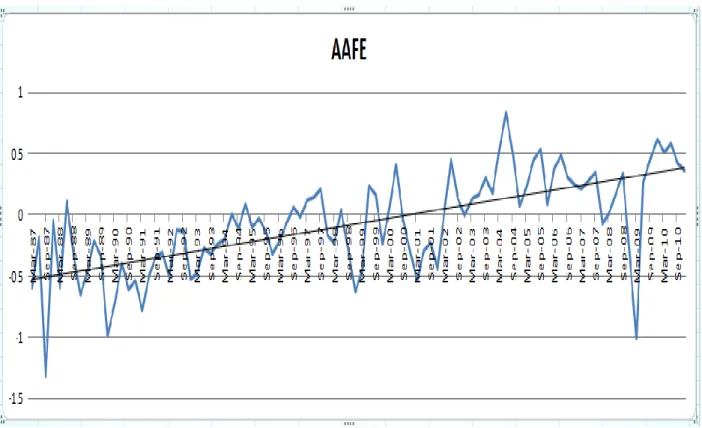
After the Global Settlement in 2003,10 analysts tend to become more conservative than
before. Figure 2.1 shows that there is an upward trend for the aggregate analyst forecast errors
during the sample period. We remove the time trend of the aggregate analyst forecast errors and
test whether the detrended aggregate analyst forecast errors are stationary. The augmented
Dickey-Fuller (ADF) test rejects the null hypothesis that the aggregate analyst forecast errors
have a unit root, suggesting the aggregate analyst forecast errors series are stationary. Hence, we
use the level of detrended aggregate analyst forecast errors to perform our analysis.
2.3.3 Economy Data
We use seasonally adjusted quarterly real gross domestic product (GDP) from Bureau of
Economic Analysis to measure the economy state. The quarterly data are in the unit of billions of
15
chained 2005 dollars. Following Næs, et al. (2011), we take the difference in the logarithm of
real GDP to measure the quarterly change in the economy, i.e.,
Figure 2.1 Aggregate Standardized Analyst Forecast Errors (AAFE) and Their Time Trend
The figure shows time-series plots of the original aggregate standardized analyst forecast errors from the sample firms in this study. The sample firms include common stocks listed on the NYSE with stock price above $1 per share, listing for the whole calendar year, and with analyst coverage. The sample period is from 1987Q1 to 2010Q4. The solid line describes the time-trend of the aggregate standardized analyst earnings forecast errors during the sample period. ) / ln( 1 t t t GDPR GDPR dGDPR (2.4)
While our focus is to examine the role of aggregate analyst earnings forecast errors in
economic forecastability of stock market liquidity, we include several control variables, which
could also be linked to the economy state. First, Fama and French (1989) document that the
default spread (yield difference between low grade bonds and high grade bonds) is high during
periods like the Great Depression when business is persistently poor and low during periods
16
(yield difference between 10-year Treasury note and 3-month Treasury bill) tends to be low near
business cycle peaks and high near troughs. Thus, they suggest that the default spread is a
long-term business condition variable, and the long-term spread as a short-long-term business cycle variable. In
our analysis, we include the term spread and the default spread as control variables.11
Also included as control variables are the market excess return and market return
volatility since stock market prices have been considered as an important leading indicator of the
economy. Following Næs, et al. (2011), we use the 3-month cumulative monthly S&P 500 index
return in excess of monthly risk-free rate as the quarterly market excess return (Mkt_Ret). As for
market return volatility, we calculate each common stock’s quarterly return volatility from daily returns for common stocks in our sample (listed on NYSE with stock price above $1 for the
whole calendar year), and then take the equally-weighted average as quarterly market volatility
(Mkt_Vol). The augmented Dickey-Fuller (ADF) tests show that all of these control variables are
stationary.
2.3.4 Summary Statistics of the Variables
Table 2.1 reports the summary statistics of the variables discussed above. During the 96
quarters from 1987Q1 to 2010Q4, the mean (and last forecast) of the aggregate standardized
analyst forecast errors (AAFE) change from negative in the first time period (1987Q1 to 1990Q4)
to positive in the last decade (2001Q1 to 2010Q4). Figure 1 plots the time series of AAFE, which
shows an obvious time trend, indicating that analysts collectively tend to exhibit more optimism
in the early period than in the later period. In the analyses that follow, we use the
detrended_AAFE to capture systematic analyst forecast errors.
17
In terms of market liquidity, the aggregate illiquidity level decreases from 0.73 in the late
80s to 0.35 from 1991 to 2000, and further decreases to 0.07 in the past decade (2001 to 2010).
The average real GDP growth rate is around 0.65% per quarter during the sample period but has
a lower growth rate of 0.41% during the past decade, compared to 0.69% during the earlier
period from 1987 to 1990 and 0.87% from 1991 to 2000. The average stock market volatility
during the sample period is around 2.46% and the overall market tends to have higher volatility
during the most recent decade. This suggests that investors tend to face more uncertainty during
the recent period than before, consistent with Campbell, et al. (2001).
The average term spread is around 1.81% during the sample period and has a higher
mean of 1.98% during the most recent decade, compared to 1.53% in the earlier period from
1987 to 1990 and 1.74% from 1991 to 2000. The average default spread is around 0.97% during
the sample period and it also has a higher mean value of 1.16% during the most recent decade,
relative to 0.75% from 1991 to 2000. The mean market excess return is around 1.02% per quarter
during the sample period, and ranges from -0.71% per quarter during the most recent decade to
2.92% per quarter from 1991 to 2000.
Table 2.2 shows the Pearson correlation coefficients between the variables. The GDP
growth rate in a quarter shows significant negative correlations with stock market liquidity
change, default spread, and market volatility in the previous quarter, but has a positive
correlation with the previous quarter’s market excess return.
These correlations suggest that stock market illiquidity, default spread, and market
volatility tend to increase (decrease) and the stock market tends to fall (rise) before economic
downturns (upturns). In short, stock market liquidity, volatility, and excess returns, and default
18
direction of the economy. Interestingly, the GDP growth rate has a significant positive
correlation of 0.45 with the concurrent detrended_AAFE(mean) and 0.43 with
detrended_AAFE(last forecast).
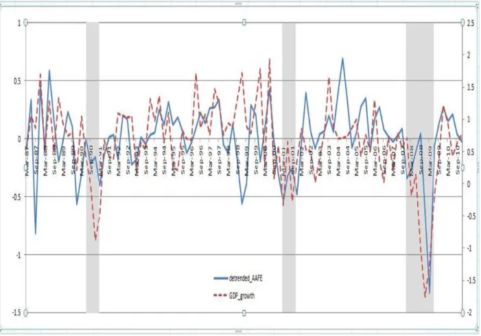
Figure 2.2 shows that there is clear comovement between these two series (GDP growth
and detrended_AAFE(mean)). Furthermore, like GDP growth, detrended_AAFE also has
significant positive correlations with term spread and market excess return in the previous
quarter and significant negative correlations with previous quarter’s default spread and market
volatility. These correlations are consistent with the notion that analyst earnings forecast errors
on individual firms contain a systematic component and that analysts collectively tend to be too
optimistic right before economic downturns, which results in negative forecast errors, and too
pessimistic right before economic upturns, which results in positive forecast errors.
It is worth pointing out that while the GDP growth has a significant negative correlation
of -0.33 with the previous quarter change in stock market liquidity, detrended_AAFE (mean)
seems to have a stronger negative correlation of -0.47 with the previous quarter change in stock
market liquidity. If the economic forecastability of stock market liquidity reflects smart
investors’ information advantages, the stronger negative correlation between detrended_AAFEt
(mean) and ILLIQt-1, along with a large positive correlation between detrended_AAFEt and
dGDPRt, provide a first hint that smart investors’ information advantages could lie on their
foreseeing and exploiting systematic analyst forecast errors. In the next section, we formally
address this issue using regression analysis.
2.4 Regression Results
This section first uses multivariate regression analyses to address two issues. First, to
19
Table 2.1 Summary Statistics of the Relevant Variables
Variables 1987Q1to2010Q4 1987Q1to1990Q4 1991Q1to2000Q4 2001Q1to2010Q4
Sample firms
ILLIQ 0.30 0.73 0.35 0.07
dILLIQ -0.0223 0.0624 -0.0499 -0.0287
Mkt_Vol 2.46% 2.36% 2.42% 2.55%
Avg_number_of_firms 1610.54 1670.75 1815.80 1381.20
Sample firms with analyst coverage (mean)
AAFE -0.0685 -0.4900 -0.1621 0.1937
detrended_AAFE -0.0004 -0.0379 0.0212 -0.0070
avg_number_of_firms 778.31 645.31 828.25 781.58
Sample firms with analyst coverage (last forecast)
AAFE 0.2176 -0.3164 0.1370 0.5118
detrended_AAFE 0.0086 -0.0814 0.0612 -0.0079
avg_number_of_firms 619.47 412.63 662.73 658.95
Sample firms with earnings information
SUE -0.0274 -0.0430 -0.0309 -0.0177 avg_number_of_firms 1271.36 1229.63 1362.50 1196.93 Economy variables GDPR 10434.19 7711.76 9436.77 12520.58 dGDPR 0.0065 0.0069 0.0087 0.0041 Term_Spread 1.81% 1.53% 1.74% 1.98% Default_Spread 0.97% 1.08% 0.75% 1.16% Mkt_Ret 1.02% 0.57% 2.92% -0.71%
This table reports the average values of the variables used in this study during the whole sample period and each sub-period. The sample firms include NYSE common stocks with stock price above $1 and listed for the whole calendar year. The sample firms with analyst coverage include the aforementioned sample firms that have I/B/E/S analyst earnings forecast data (summary history and detail history) available. The standardized aggregate analyst forecast error of a firm in a given quarter is the difference between actual earnings and estimated earnings from analysts standardized by the previous eight quarters’ standard deviation of the difference. The aggregate standardized analyst forecast error, AAFE, is the equally-weighted average across the sample firms with analyst coverage. The detrended aggregate standardized analyst forecast error, detrended_AAFE, removes the time trend of the original series during the sample period. Mean is from summary history and last forecast is from detail history. SUE uses the actual earnings reported 4 quarters before as the benchmark. ILLIQ is the average illiquidity measure of Amihud (2002) across the sample firms, and dILLIQ is the logarithm difference between the current quarter’s and the previous quarter’s
20 (Table 2.1 continued)
is the real GDP is in billions of chained 2005 dollars, and dGDPR is real GDP growth, measured by the logarithm difference between the current quarter’s and the previous quarter’s GDPR. Term_Spread is the yield difference between 10-year Treasury note rate and 3-month Treasury bill rate; and Default_Spread is the difference between Moody’s Baa bond yield and Moody’s Aaa bond yield. Mkt_Ret is the market excess return proxied by the 3-month cumulative monthly excess return between S&P 500 index return and the risk-free rate.
Table 2.2 Correlation Matrix detrended_AAFEt
(mean)
detrended_AAFEt
(last forecast) ASUEt dILLIQt-1 Term_Spreadt-1 Default_Spreadt-1 Mkt_Rett-1 Mkt_Volt-1
dGDPRt 0.4475 (<.0001) 0.4323 (<.0001) 0.3880 (<.0001) -0.3341 (0.0009) 0.0114 (0.9122) -0.4685 (<.0001) 0.3547 (0.0004) -0.4113 (<.0001) detrended_AAFEt (mean) 0.7591 (<.0001) 0.6152 (<.0001) -0.4714 (<.0001) 0.2172 (0.0335) -0.3583 (0.0003) 0.3813 (0.0001) -0.4883 (<.0001) detrended_AAFEt (last forecast) 0.4355 (<.0001) -0.4206 (<.0001) 0.0536 (0.6038) -0.4133 (<0.0001) 0.3435 (0.0006) -0.3915 (<.0001) ASUEt -0.3791 (<.0001) -0.0383 (0.7113) -0.6275 (<.0001) 0.3024 (0.0028) -0.6715 (<.0001) dILLIQt-1 -0.0644 (0.5329) 0.3511 (0.0005) -0.4159 (<.0001) 0.5272 (<.0001) Term_Spreadt-1 0.2689 (0.0081) -0.0354 (0.7323) 0.1401 (0.1733) Default_Spreadt-1 -0.2928 (0.0038) 0.7262 (<.0001) Mkt_Rett-1 -0.4441 (<.0001)
This table shows the Pearson correlation coefficients between variables used in the analysis. The associated p-values are reported in parentheses below each correlation coefficient. dGDPRt is the logarithm difference between current real GDP and previous real GDP. detrended_AAFEt is the aggregate standardized
analyst forecast error series taken out time trend. ASUEtis the aggregate standardized earnings surprises. The following variables are from previous quarter. For
the following lagged variables, dILLIQt-1 is the logarithm difference between current aggregate liquidity level and previous aggregate liquidity level.
Term_Spreadt-1is the yield difference between 10-year Treasury note and 3-month Treasury bill. Default_Spreadt-1is the yield difference between Moody’s Baa
and Moody’s Aaa. Mkt_Rett-1is the 3-month cumulative S&P500 monthly return and risk-free rate difference. Mkt_Volt-1is the equal-weighted 3-month stock
21
Second, could changes in stock market liquidity be linked to predicted aggregate analyst
forecast errors? Addressing the issues help us connect the notions that changes in stock market
liquidity reflect smart investors’ trading behavior and that smart investors take advantage of
predicted analyst forecast errors. The analyses provide a basis for us to further test our
hypothesis that the economic forecastability of stock market liquidity is through systematic
analyst forecast errors. We focus on the results from summary history of I/B/E/S (mean) and also
report results from detail history (last forecast) and standardized earnings surprises.
Figure 2.2 Detrended Aggregate Analyst Forecast Errors (detrended_AAFE) and GDP Growth
The figure shows the trends of two time series from 1987Q1 to 2010Q4: detrended standardized aggregate analyst forecast errors and GDP growth. We take out the linear time trend from the original standardized aggregate analyst forecast errors to get the detrended series, and take the logarithm difference between the current real GDP and previous quarter’s real GDP number to get the GDP growth series. The left axis is for the detrended aggregate standardized analyst forecast errors and the right axis is for the GDP growth. The shaded areas mark the following three NBER recessions: July 1990-March1991, March 2001-November 2001, and December 2007-June 2009.
22 2.4.1 Predicting Aggregate Analyst Forecast Errors
To examine the predictability of aggregate analyst forecast errors, we use the following
regression model: 0 1 1 2 1 3 1 4 1 _ * _ * _ * _ * _ t t t t t t
detrended AAFE b b Mkt Vol b Term Spread
b Default Spread b Mkt Ret
(2.5)
Table 2.3 reports the regression results, which show that detrended_AAFEt is significantly and
negatively related to lagged stock market volatility, and significantly and positively related to
lagged term spread and lagged market excess returns. The results suggest that analysts
collectively tend to be too optimistic when stock market returns are lower and more volatile and
when term spread is smaller, and that, conversely, they tend to be too pessimistic when stock
market returns are higher and less volatile and when term spread is larger. The adjusted-R2 of
the regression in (2.5) is 0.33, suggesting that about one third of the variation in aggregate
analyst forecast errors is predictable.
Based on the results in Table 2.3, we obtain the predicted aggregate analyst forecast error
in time t as
t-1 t t-1 t-1
t-1 t-1
E (detrended_AAFE )= 0.28 - 13.68* Mkt_Vol +7.84* Term_Spread
-9.31* Default_Spread +0.71* Mkt_Ret (2.6)
and the residual part as
t t t-1 t
residual_detrended_AAFE = detrended_AAFE - E (detrended_AAFE ) (2.7)
If smart investors exploit systematic analyst forecast errors, the predictable part of aggregate
analyst forecast errors is likely to be more useful than the unpredictable part to smart investors.
Indeed, Table 2.4 shows that stock market liquidity, dILLIQt1, is strongly associated with
t t-1
23
The strong association between changes in stock market liquidity and predicted
detrended_AAFE and the strong correlation between real GDP growth and aggregate analyst
forecast errors reported earlier lead us to consider that the source of the economic forecastability
of stock market liquidity may lie in analyst forecast errors. We next turn to explore this issue.
2.4.2 The Source of the Economic Forecastability of Stock Market Liquidity
We use the following regression model to compare the link strength to real GDP growth,
,
t
dGDPR of changes in stock market liquidity to that of predicted aggregate analyst forecast
errors:
t 0 1 t-1 2 t-1 3 t-1 t t
dGDPR = b +b * dILLIQ +b * dGDPR +b * E (detrended_AAFE )+e (2.8)
Similar to Naes, Skjeltorp, and Odegaard (2011), Table 2.5 shows that, without
t t-1
E (detrended_AAFE ) in the regression model, dGDPRt is negatively related to dILLIQt1,
with a Newey-West corrected t-value of -2.65. This confirms the stock market liquidity’s
economic forecastability in our sample period from 1987 to 2010. However, in the presence of
t t-1
E (detrended_AAFE ), dGDPRt is no longer significantly related to dILLIQt1 since its
Newey-West corrected t-value becomes -1.22. Instead, dGDPRt is significantly related to
t t-1
E (detrended_AAFE ), with a Newey-West corrected t-value of 2.85. The results suggest that
while stock market liquidity contains useful information for forecasting future economic activity,
this information content of stock market liquidity is largely encompassed by predicted aggregate
analyst forecast errors. Thus, the evidence is consistent with our hypothesis that stock market
liquidity as an economic leading indicator is built on systematic analyst forecast errors.
To further illustrate our point, we decompose real GDP growth into two components: one
24
Table 2.3 Predicting Aggregate Analyst Forecast Errors
Panel A: Analyst Earnings Forecast Errors from Summary History of I/B/E/S
Dependent Variable Constant Mkt_Vol
t-1 Term_Spreadt-1 Default_Spreadt-1 Mkt_Rett-1 Adjustedj_R
2 detrended_AAFEt (mean) 0.47*** -19.14*** 0.2303 (4.25) (-4.06) detrended_AAFEt (mean) 0.37*** -17.48*** 7.93*** -8.50 0.3057 (3.86) (-2.71) (3.52) (-0.74) detrended_AAFEt (mean) 0.28*** -13.68** 7.84*** -9.31 0.71*** 0.3311 (2.76) (-2.07) (3.45) (-0.85) (2.82)
***, **, * significant at the 1%, 5%, and 10% level, respectively.
Panel B: Analyst Earnings Forecast Errors from Detail History of I/B/E/S
Dependent Variable Constant Mkt_Vol
t-1 Term_Spreadt-1 Default_Spreadt-1 Mkt_Rett-1 Adjustedj_R
2 detrended_AAFEt (last forecast) 0.32*** -12.49*** 0.1443 (3.34) (-3.28) detrended_AAFEt (last forecast) 0.27*** -5.54 3.47 -19.44* 0.1887 (3.50) (-0.92) (1.29) (-1.78) detrended_AAFEt (last forecast) 0.19*** -2.14 3.39 -20.16** 0.64*** 0.2197 (2.46) (-0.37) (1.28) (-2.01) (2.84)
25 (Table 2.3 continued)
Panel C: Standardized Earnings Surprises
Dependent Variable Constant Mkt_Vol
t-1 Term_Spreadt-1 Default_Spreadt-1 Mkt_Rett-1 Adjustedj_R
2 ASUEt 0.78*** -32.68*** 0.4450 (3.78) (-3.70) ASUEt 0.73*** -21.57*** 3.62 -30.42** 0.4881 (4.95) (-2.79) (1.07) (-2.40) ASUEt 0.72*** -21.24*** 3.61 -30.11** 0.06 0.4827 (5.08) (-2.77) (1.06) (-2.41) (0.21)
***, **, * significant at the 1%, 5%, and 10% level, respectively.
The table reports the results of regressing detrended aggregate analyst forecast errors on lagged macro variables. The model estimated is
.
t 0 1 t-1 2 t-1 3 t-1 4 t-1 t
detrended_AAFE = b +b * Mkt_Vol +b *Term_Spread +b * Default_Spread +b * Mkt_Ret +e
The explanatory variables include market volatility, term spread, default spread, and market excess return. The Newey-West corrected t-statistics (Bartlett kernel
with a lag length of 2) are reported in parentheses below the coefficient estimates.
Table 2.4 Aggregate Analyst Forecast Errors and Stock Market Liquidity Changes
Panel A: Analyst Earnings Forecast Errors from Summary History of I/B/E/S
Dependent variable Constant dILLIQ
t-1 Adjustedj_R2 Et-1(detrended_AAFEt) (mean) -0.0065 (-0.30) -0.3607*** (-3.31) 0.2994 residual_dtrended_AAFEt (mean) -0.0026 (-0.10) -0.1516* (-1.81) 0.0201
26 (Table 2.4 continued)
Panel B: Analyst Earnings Forecast Errors from Detail History of I/B/E/S
Dependent variable Constant dILLIQ
t-1 Adjustedj_R 2 Et-1(detrended_AAFEt) (last forecast) 0.0048 (0.31) -0.2279** (-2.54) 0.2553 residual_dtrended_AAFEt (last forecast) -0.0024 (-0.09) -0.1439** (-2.21) 0.0295
***, **, * significant at the 1%, 5%, and 10% level, respectively.
Panel C: Standardized Earnings Surprises
Dependent variable Constant dILLIQ
t-1 Adjustedj_R 2 Et-1(ASUEt) -0.0356 (-0.98) -0.4879** (-2.30) 0.2513 residual_ASUEt -0.0004 (-0.01) -0.02365 (-0.15) -0.0100
***, **, * significant at the 1%, 5%, and 10% level, respectively.
The table reports the results of regressing the two components (predicted and residual) of detrended aggregate analyst forecast errors on stock market liquidity changes from 1987 Q1 to 2010 Q4. The regression model used to get the predicted component of detrended aggregate analyst forecast errors,
t-1 t
E (detrended_AAFE ), is reported in table 2.3:
t 0 1 t-1 2 t-1 3 t-1 4 t-1 t
detrended_AAFE = b +b * Mkt_Vol +b *Term_Spread +b * Default_Spread +b * Mkt_Ret +e
And the residual component is
.
t t t-1 t
residual_detrended_AAFE = detrended_AAFE - E (detrended_AAFE )
27
That is, based on the regression model,
t 0 1 t t
dGDPR = b +b * detrended_AAFE +e (2.9)
the related component is AAFE_related_dGDPR = b +b * detrended_AAFEt ˆ0 ˆ1 t and the
unrelated component is residual dGDPR_ tdGDPRtAAFE related dGDPR_ _ t.
If systematic analyst forecast errors contain all the relevant information for the economic
forecastability of stock market liquidity, then we expect that stock market liquidity has predictive
power on AAFE related dGDPR_ _ t, but not on residual dGDPR_ t.
Indeed, Table 2.6 shows that AAFE related dGDPR_ _ t is significantly and negatively
related to dILLIQt1 and that the predictive power of dILLIQt1 remains after controlling for
market volatility, term spread, default spread, and market excess returns. However, Table 2.6
also shows that residual dGDPR_ t has virtually no relation with dILLIQt1,suggesting that
1
t
dILLIQ has no predictive power on residual dGDPR_ t. The results validate that systematic analyst forecast errors possess all the pertinent information for stock market liquidity as an
economic leading indicator.
2.5 Conclusion
This paper extends Næs, Skjeltorp, and Ødegaard’s (2011) study to better understand the
mechanism for stock market liquidity to have the economic forecastability. According to Næs, et
al. (2011), our empirical results show that the reason that stock market liquidity contains useful
information for inferring the future state of the economy is because changes in stock market
liquidity can capture smart investors’ flight-to-quality behavior in which smart investors sell
risky and hard-to-dispose securities before economic downturns, and buy them before economic
28
Our inquiry starts with a simply question: Why are other investors willing to buy (sell)
risky and hard-to-dispose securities when smart investors sell (buy) them before economic
downturns (upturns)? The question leads us to consider that while analyst earnings forecasts
provide useful information to market participants and help them form market expectations, smart
investors may foresee and exploit systematic analyst forecast errors. If systematic analyst
forecast errors are correlated with economic conditions, stock market liquidity, by capturing
smart investors’ collective behavior on analyst forecast errors, could become informative on changes in the economy.
Thus, we hypothesis that analyst earnings forecast errors have a systematic component,
which is predictable and related to changes in the economy, and that smart investors exploit
analyst forecast errors, which leads to the economic forecastability of stock market liquidity.
Consistent with our hypothesis, we find that there is a strong correlation between detrended
aggregate analyst forecast errors and concurrent GDP growth and that a large part of the forecast
errors can be predicted using lagged macro variables. Furthermore, once we control for the
predictable forecast errors, the economic forecastability of stock market liquidity disappears. In
sum, our analysis reveals that aggregate analyst forecast errors are very informative on business
cycle. They contain all the relevant information for stock market liquidity as an economic
leading indicator. Smart investors foresee changes in economy unexpected by analysts and trade
upon this private information, causing changes in stock market liquidity. Hence, we observe a
relationship between stock market liquidity and business cycle. Specifically, smart investors sell
stocks before the general investment public knows the economy is worsening and before a
recession starts, and they buy stocks before the general investment public knows the economy is
29
Table 2.5 GDP Growth Rate, Stock Market Liquidity Change, and Predicted Aggregate Analyst Forecast Error
Dependent variable Constant dILLIQt-1 dGDPRt-1 Et-1(AAFEt)(mean) Adjustedj_R
2 dGDPRt 0.0014*** (2.58) 0.4564*** (2.97) 0.2000 dGDPRt 0.0040*** (3.30) -0.0048*** (-2.65) 0.3908*** (2.99) 0.2334 dGDPRt 0.0046*** (4.00) 0.3007** (2.31) 0.0110*** (3.69) 0.2686 dGDPRt 0.0046*** (4.08) -0.0022 (-1.22) 0.2963** (2.29) 0.0092*** (2.85) 0.2671
Dependent variable Constant dILLIQt-1 dGDPRt-1 Et-1(AAFEt)(last) Adjustedj_R
2 dGDPRt 0.0050*** (4.47) 0.2147 (1.65) 0.0207*** (4.51) 0.3004 dGDPRt 0.0049*** (4.55) -0.0018 (-1.06) 0.2143 (1.66) 0.0186*** (3.83) 0.2976
Dependent variable Constant dILLIQt-1 dGDPRt-1 Et-1(ASUEt) Adjustedj_R2
dGDPRt 0.0050*** (4.20) 0.2616* (1.97) 0.0078*** (4.07) 0.2631 dGDPRt 0.0050*** (4.21) -0.0026 (-1.32) 0.2604* (1.98) 0.0064*** (2.99) 0.2654
***, **, * significant at the 1%, 5%, and 10% level, respectively.
This table reports the result of regressing GDP growth rate, dGDPRt, on lagged stock market liquidity change, dILLIQt1, and the predicted component of the aggregate analyst forecast error, E (detrended_AAFE )t-1 t ,obtained from the regression results reported in Table 2.3. The model is
0 1* 1 2* 1 3*
t t t t-1 t t
dGDPR b b dILLIQ b dGDPR b E (detrended_AAFE )
30
Table 2.6 Stock Market Liquidity and the Components of GDP Growth
Panel A: Analyst Earnings Forecast Errors from Summary History of I/B/E/S
Dependent variable Constant dILLIQ
t-1 Mkt_Volt-1 Term_Spreadt-1 Default_Spreadt-1 Mkt_Rett-1 Adjustedj_R
2 AAFE_related_dGDPRt (mean) 0.0064*** (21.44) -0.0048*** (-3.29) 0.2140 AAFE_related_dGDPRt (mean) 0.0084*** (9.40) -0.0021** (-2.24) -0.0929 (-1.54) 0.0665*** (3.05) -0.0877 (-0.91) 0.0051** (2.37) 0.3547 residual_dGDPRt -0.0001 (-0.07) -0.0028 (-1.23) 0.0083 residual_dGDPRt 0.0025 (1.37) -0.0003 (-0.14) 0.1122 (1.06) -0.0017 (-0.04) -0.5454*** (-2.81) 0.0100 (1.52) 0.0922
***, **, * significant at the 1%, 5%, and 10% level, respectively.
Panel B: Analyst Earnings Forecast Errors From Detail History of I/B/E/S
Dependent variable Constant dILLIQ
t-1 Mkt_Volt-1 Term_Spreadt-1 Default_Spreadt-1 Mkt_Rett-1 Adjustedj_R
2 AAFE_related_dGDPRt (last forecast) 0.0065*** (19.85) -0.0041*** (-3.33) 0.1681 AAFE_related_dGDPRt (last forecast) 0.0077*** (7.80) -0.0024** (-2.40) 0.0154 (0.23) 0.0300 (1.02) -0.2242** (-2.11) 0.0053** (2.21) 0.2532