NBER WORKING PAPER SERIES
BIDDER DISCOUNTS AND TARGET PREMIA IN TAKEOVERS
Boyan Jovanovic Serguey Braguinsky
Working Paper9009
http://www.nber.org/papers/w9009
NATIONAL BUREAU OF ECONOMIC RESEARCH 1050 Massachusetts Avenue
Cambridge, MA 02138 June 2002
We thank Luis Cabral, Masako Ueda, and the Finance Lunch group at the GSB of the University of Chicago for helpful comments. The views expressed herein are those of the authors and not necessarily those of the National Bureau of Economic Research.
© 2002 by Boyan Jovanovic and Serguey Braguinsky. All rights reserved. Short sections of text, not to exceed two paragraphs, may be quoted without explicit permission provided that full credit, including © notice, is given to the source.
Bidder Discounts and Target Premia in Takeovers Boyan Jovanovic and Serguey Braguinsky
NBER Working Paper No. 9009 June 2002
JEL No. G3
ABSTRACT
When a takeover is announced, the sum of the stock-market values of the firms involved often falls, and the value of the acquirer almost always does. Does this mean that takeovers do not raise the values of the firms involved? Not necessarily. We set up a model in which the equilibrium number of takeovers is constrained efficient. Yet, upon news of a takeover, a target's price rises, the bidder's price falls, and, most of the time the joint value of the target and acquirer also falls.
Boyan Jovanovic Serguey Braguinsky
Department of Economics The George Stigler Center
University of Chicago Walker Hall
1126 E. 59th St. University of Chicago
Chicago, IL 60637 Chicago, IL 60637
and NBER serguey@uchicago.edu
Bidder Discounts and Target Premia in Takeovers
∗
Boyan Jovanovic
†and Serguey Braguinsky
‡June 3, 2002
Abstract
When a takeover is announced, the sum of the stock-market values of the
firms involved often falls, and the value of the acquirer almost always does. Does this mean that takeovers do not raise the values of thefirms involved? Not necessarily. We set up a model in which the equilibrium number of takeovers is constrained efficient. Yet, upon news of a takeover, a target’s price rises, the bidder’s price falls, and, most of the time the joint value of the target and acquirer also falls.
1
Introduction
On news of a takeover, the share price of the targetfirm usually rises sharply, while that of the acquiringfirm usually falls. The joint value may or may not rise. Surveying thefield, Andrade, Mitchell and Stafford (2001) report that since 1973 target premia were 20 or 30 percent, acquirer discounts were minus 3 or 4 percent, and that the joint value shows no clear pattern. They conclude (p. 118) that “the fact that mergers do not seem to benefit acquirers provides a reason to worry ...[that mergers do not raise value].” To explain such evidence (Shleifer and Vishny 2001) have assumed that investors are irrational and (Roll 1986) has assumed that managers use takeovers to extend their empires at the expense of the shareholder. The evidence about the bidder discount and joint discount has been taken to imply that takeovers often just redistribute rents from acquirers to their targets or that they even destroy rents.
We show, however, that even when investors are rational, when agency problems are absent, and when mergers do create value, the acquirer’s value and even the joint value of the bidder and target may fall when a takeover is announced. The bidding
firm’s value falls because its bid reveals that its internal investment opportunities are
∗We thank Luis Cabral, Masako Ueda, and the Finance Lunch group at the GSB of the University
of Chicago for helpful comments.
†NYU and the University of Chicago.
poor. The target’s value rises because an acquisition signals that the target’s internal investment opportunities are good. A takeover benefits both parties, and the number of takeovers is, in a sense, constrained-efficient. And yet the bidder discount usually outweighs the target premium so that the joint value drops.
We discuss other related work later on in the paper; the highlights there are Holmes and Schmitz (1990, 1995), Campa and Kedia (forthcoming), Villalonga (2001), Gort, Grabowski, and McGuckin (1985), and Myers and Majluf (1984). But first we present the model and then discuss its robustness.
2
Model
In the model that we are about to describe, takeovers are the mechanism that moves good projects from bad managers to good managers. At the outsetfirms differ in the quality,x, of their management.1 Each firm then draws a project and the quality,z,
of projects, too, differs over firms. Some good managers end up with bad projects and vice versa. Takeovers then serve to shift the good projects from bad managers to good managers. Afirm’s output is
xz. (1)
Thus the quality of a project, z, and the firm’s ability to implement a project, x, are complements. Among firms, x ≥ 0 is distributed according to the cumulative distribution functionF (x). Projects are either good or useless: z ∈{0,1}. A fraction
λ of projects is good, and the fraction 1−λ is useless.
A firm cannot change the quality of its management. It can, however, acquire another firm and manage its project. A manager can handle only one project. If a
firm (x, z) buys firm (x0, z0), it then uses its own management, x, and the project,
z0, of thefirm that it has acquired. It drops its own, useless project, and lets go the
manager of the target. The output of the merged entity will be2
xz0. (2)
To an acquirer, then, only the target’sz0 matters. The departing manager receives
no severance payment and does not stand in the way of the takeover as long as it
1Andrade et al (2001) and Jovanovic and Rousseau (2002) report evidence that acquisitions are
disproportionately made by high-Qfirms.
2This partially reflects findings by McGuckin and Ngyen (1995) and Schoar (2000) that the
productivity of the target’s plants rises (in this case fromx0 tox) while that of the acquirer’s plants falls (in this case fromzto zero as the plant is ‘abandoned’). We re-visit this issue in Section 4. The mergedfirm produces more output than the combined stand-alone outputs of the twofirms. Hence, productivity rises after a merger. Lichtenberg and Siegel (1987) find that plants changing owners had lower initial levels of productivity and higher subsequent productivity growth than plants that did not change hands.
benefits the shareholders of his firm. We assume that all mergers are driven only by the prospect of real gain, all investors are rational and all managers act only in the long-term interests of shareholders. This is not to suggest that, empirically, mergers are always exactly like that. Rather, we assume that all mergers create value, that the stock market is efficient, and that there is no agency problem, in order to see exactly where these extreme assumptions lead.
2.1
A sketch of equilibrium
We begin with an intuitive derivation of the equilibrium takeover activity and of the price, q, of targets.
The supply of targets.–Let us start off by assuming as a constraint something that will later emerge as an equilibrium action; namely, that, before it can be taken over, afirm must certify that its z = 1. The total mass of potential targets isλ. The act of certifying the quality of its project costs the firm c. If the firm does not wish to be a target and if, instead, it were to manage its own project, its payoffwould be
x. Thus the direct plus the foregone-earnings costs of being a target arec+x.Thus, at a price of q, the number of willing targets would be all the z = 1 firms for which
c+x is less than q. That number is
λF(q−c)≡S(q).
Evidently, S(q) is an upward sloping supply curve that is continuous if F is.
The demand for targets.–Any firm that drew a project z = 0 is a potential acquirer. Unless it manages to acquire anotherfirm, thisfirm faces a revenue of zero. The number of such firms is 1−λ. If firm x manages to buy another firm with a certified z = 1 project, its revenue will be x. Thus, at a price of q, the number of willing acquirers would be the z = 0 firms for which x−q is positive. That number is
(1−λ) [1−F (q)]≡D(q),
a downward sloping demand curve.
Figure 1 shows the equilibrium price of targets qE and number of takeovers TE, where the two curves intersect. Atq = 0, all the 1−λ firms withz = 0 projects are willing to buy, hence the demand curve cuts the horizontal axis at the point1−λ. As
q gets large, all the λ firms withz = 1 projects are willing to sell, and so the supply curve approaches λ. Rents are split between the targets and the acquirers, with the largest rents in each group going to the highest-x acquirers and the lowest-xtargets. Figure 1 relates to a stage of the game at which most of the uncertainty has been resolved. It says nothing about bidder discounts and target premia. Here now is a more precise account of the game.
S(q) 1 - λ λ D(q) c qE
Price
of
targets
Number of
takeovers
TEFigure 1: Supply and Demand for Targets
2.2
The
fi
ve stages of the game
We shall treat all takeovers as cash sales although this is done purely for expositional reasons. The dividends of the combined entity are then paid to the shareholders of the acquiringfirm. Shareholders are risk neutral and they hold on to their shares until the firm pays its dividend and liquidates or until it is bought by another firm. We assume that a manager acts in the shareholder’s interest. That is, he puts thefirm up for sale if the cash payment,q, exceeds hisfirm’s stand-alone dividend. Alternatively, the manager buys anotherfirm if the dividend he can secure his original shareholders net of the cash paid for the acquiredfirm, exceeds his firm’s stand-alone dividend.
Events occur infive stages:
1. Firms form. Based on its x(which is public knowledge) eachfirm is sold at its Stage-1 pricep(x).
2. Thefirm privately observesz. It may (thruthfully) disclose its z to everyone at a cost c.3
3In reality there is a whole set of indicators of project quality, and each of them probably carries
a differentc. Grayet al (1990, Table 1) report 33 of them. Firms seem to favor disclosing of their major new products and major capital expenditure projects in progress, but do not favor disclosing their major patents.
3. Firm may enter the takeover market as a buyer or a seller.4
4. Based on its Stage-2 and Stage-3 choices, thefirm’s price takes on its “Stage-4” level. (It is to this stage that Figure 1 relates)
5. The firm pays its dividend and liquidates.
2.3
Stage-3 actions and Stage-4 prices
Equilibrium.–Key to equilibrium is a pair of real numbers,x0, andx1, wherex0 < x1. These two numbers divide the set ofx’s into three regions — top, middle, and bottom. Targets come from the bottom region, acquirers from the top region. Firms from the middle region stay out of the takeover market. We start describing the equilibrium with an account of the Stage-3 actions and Stage-4 prices of thefirms in each region.
The bottom region — x≤x0.–If such afirm drawsz = 1, it discloses that fact. It becomes a takeover target and sells at the priceq. All targets sell at the same price.5
Firm x0 is indifferent between disclosing z (and getting its shareholders a payoff of
q−c), and not disclosing and managing its own project (and getting its shareholders a payoffof x0). That is,
q−c=x0. (3)
If such a firm does not disclose itsz, the market rationally infers that any firm with
x < x0 that has not disclosed is a z = 0 firm. The Stage-4 price of such a firm is zero. To sum up, then, in the bottom region, afirm’s Stage-4 price is q if z = 1, and it is zero ifz = 0.
The middle region —x∈(x0, x1).–Such afirm does not disclose itsz and it does not bid for other firms. The market infers nothing from its inaction. If such a firm has z = 1, it can guarantee its shareholders more than q−c, and it would refuse (and successfully repel) any takeover bid at the price q. If, on the other hand, such a firm has z = 0, buying another firm at the price q would leave it with a negative net payoff. Thus, if a firm from this region did not refuse a takeover bid, it would reveal itself to be a “lemon”. Thus no one bids forfirms in this region and their prices remain unchanged atλx.
4I.e., afirm can repel an unwanted bid. Of all takeover bids, only 8.3% of all bids are hostile and
only 4.4% eventually succeed (Andradeet al, 2001). We do not explain such mergers.
5Strictly speaking, disclosure should occur before the takeovers announcement. Certainly the
price of the target-to-be does rise a bit before the takeover announcement (Pound and Zeckhouser 1990). Firms must, in fact, disclose business plans and other trade secrets at the IPO stage, and when taking out patents. Many firms are taken over during the several months’ waiting period between an IPOfiling and SEC approval. Some are taken over precisely for their intellectual prop-erty, i.e., their patents. The direct costs of such disclosures may be small, but they may help the
firm’s competitors and any profits thus foregone should also be a part of c. Firms seem to regard ‘competitive disadvantage’ as the largest part ofc(Gray et al 1990, Table 4).
q
q - c
Prices
x
0x
1x
x - q
x
45
λ
x
targets
bidders
Figure 2: Stage-4 Prices
The top region —x≥ x1.–Afirm that has drawnz = 0 has spare capacity in its organization capital x that it will seek to employ. Such a firm buys a discloser from the first region thereby raising its own output and dividend from zero to x; and its Stage-4 price is x−q. The lowest-quality bidder x1 is indifferent between bidding (and getting a payoffofx1−q), and managing its own project (and getting zero), so that
q =x1. (4)
If it does not bid, this signals to the market that the firm’s z = 1, and its Stage-4 price isx.
Why don’t the z = 0 firms refrain from bidding and thereby secure a jump in their price? Because it then would deliver a zero dividend to its shareholders who are following a “buy and hold” strategy.6 To sum up, then, in the top region, a firm’s
Stage-4 price is x if z = 1, and x−q if z = 0. These Stage-4 prices are depicted by heavy lines in Figure 2. In the middle region there is just one heavy line because, at stage-4, the market cannot distinguish the good firms from the lemons. In the other two regions, the actions of the firms have fully revealed their type.
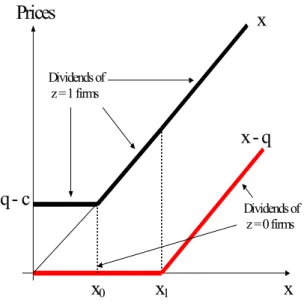
The discontinuities in the price-functions of Figure 2 are misleading; the share-holders of the good firms receive a continuous payoff as we raise x, and so do the shareholders of the badfirms. The situation is illustrated in Figure 3. Now the gains
6If enough shareholders were to sell their shares at Stage 4, and if the manager wanted to
maximizeinterim shareholder utility, he would refrain from bidding and masquerade asz= 1firms. Other shareholder holding strategies may inducez= 0firms to not bid.
q - c Prices x0 x1 x x - q x Dividends of z = 1 firms Dividends of z = 0 firms
Figure 3: How Equilibrium Dividends Depend on xand z
to trade are apparent; in the absence of takeovers, the z = 1 firms would be paying their shareholders a dividend of x (i.e., the 450 line), and the z = 0 firms would be paying their shareholders a dividend of zero (i.e., the horizontal axis). But what we end up with is a Pareto improvement, with the targets and the bidders doing strictly better than they would if there were no trade.
Market clearing.–The Stage-4 prices must guarantee that the takeover market clears, i.e., that the demand for targets equals their supply:
λF(q−c) = (1−λ) (1−F [q]) (5)
so that we are at an intersection of the two curves in Figure 1.
2.4
Stage-1 prices,
p
(
x
)
For firms in the middle region the Stage-1 prices are the same as the Stage-4 prices, namely,λx. In the two other regions, a firm’s Stage-1 price is a weighted sum of the prices it will fetch at stage 4, the weights being the probabilities of z being zero and one. The stage-1 prices are:
p(x) = λ(q−c) if x≤x0, λx if x∈(x0, x1), λx+ (1−λ) (x−q) if x≥x1. (6)
Since there are no aggregate shocks, the value of the stock market as a whole is the same at Stage 4 as it is at Stage 1. But the dispersion of prices is higher at Stage 4.
2.5
Existence of a positive-takeover equilibrium
Trade infirms stems from differences in comparative and absolute advantage in man-agement, i.e., from the dispersion inx’s. Letxmin be the smallest andxmaxthe largest value of x in the support of F. If the range ofx is larger than c, takeovers will take place in equilibrium.
Proposition 1 (Existence) If F is continuous, if 0< λ <1, and if
c < xmax−xmin, (7)
then takeovers do occur in equilibrium,
x1 =x0+c (8)
and q∈(c, xmax) uniquely solves
λF(q−c) = (1−λ) (1−F [q]). (9)
Proof. Solving (3) for q and substituting into (4) implies that if equilibrium exists, (8) must hold. Eq’s (3), (4), and (5) imply (9). It remains to be shown that, for each λ and c, (9) has a unique solution for q. This follows in 2 steps: (i) at
q = xmax the RHS of (9) is zero whereas, by (7), the left-hand side of (9) is strictly positive and(ii) atq =cthe opposite is true. Since the LHS of (9) is continuous and increasing inq whereas the RHS is continuous and decreasing, we are done.
2.6
Comparative statics
The parameters of the model arec,λ, andF. The conditions of the existence theorem provide clues to how the solution changes when the parameters change. Condition (7) emphasized that takeovers are driven by the dispersion of x’s, summarized by their range — no takeovers can occur if (7) fails. But the theorem also requires that there be dispersion in thez’s; if all firms had the same-quality projects (which would happen if λ = 0 or λ = 1), again there would be no takeovers. The number of equilibrium takeovers is therefore non-monotonic in λ. Finally, takeover activity declines withc. Formally, differentiation of (9) reveals that
∂q
∂λ <0 and
∂q
∂c >0. (10)
When λ is high, there are more good projects in total and the demand for targets falls relative to their supply and, hence, so does q. On the other hand, when it costs more to disclose quality, the price of targets will rise so as to reflect that fact. Eq’s (4) and (10) imply that
∂x1
∂λ <0 and
∂x1
so that the number of takeovers, (1−λ) [1−F (x1)] decreases with c. Eq’s (3) and (10) imply that ∂x0 ∂λ <0, and ∂x0 ∂c <0, (12)
this latter because we just established that the number of takeovers, which also equals
λF(x0), decreases with c.
2.7
Discounts and premia
At Stage 4, all targets trade at a premium over their Stage-1 prices, and all bidders trade at a discount. We measure the premia and discounts as percentages of Stage-1 prices p(x).
The target premium.–From (6), the premium is
(q−c)−p(x) p(x) = (1−λ) (q−c) λ(q−c) = 1−λ λ ,
and it is the same for all targets. The target premium is high when good projects are scarce and when, as a result, a disclosure that z = 1 is especially good news. Since target premia are on average about 0.2, the relevant value seems to be λ≈0.83.
The bidder discount.–Conversely, the bidder discount is high when good projects are plentiful and when, as a result, the revelation of z = 0 that is implicit in afirm’s decision to acquire another, is especially bad news. The discount is smaller for the high-x bidders because all bidders pay the same price, q, but the high-x bidders benefit more. The absolute value of bidder’s discount, i.e., the fraction of value lost upon announcement, is
δ(x)≡ λq
x−(1−λ)q.
From (4) x1 =q, and so δ(x1) = 1; the marginal bidder loses all of his value. As x
rises, the discount steadily shrinks and converges to zero as x gets large.
The values combined.–The target’s x’s do not affect their prices at any stage. Therefore only the acquirer’s xaffects the sum of the two firms’ Stage-1 and Stage-4 prices. Relative to the sum of the twofirms’ ex-ante values, the ex-post “joint” value of the merged firm is
J(x) = x−c
q(2λ−1) + (x−λc), (13)
an expression that is relevant for x≥x1 only. The next proposition reports a result that we shall use later: Forλ ≥1/2, the joint values drop:7
7The model also impies a rise in the price of the non-bidders with x > x1. This “non-bidder
premium” is
x−p(x)
p(x) =
(1−λ)x1 λx+ (1−λ) (x−x1).
Proposition 2 (Joint values). For any c, J(x) is strictly increasing in x if λ ≥
1/2 and
J(x)<1 for all (c, x) and all λ≥1/2. (14)
Proof. Thefirst claim follows immediately from (13). As for (14), the right-hand side of (13) is less than unity when λ = 1/2 and it is even smaller when λ > 1/2
because q >0.
Since it does not involve x, (14) applies to the joint value of all takeovers. The drop is smaller for the high-x firms.
In all cases, including those in which the joint value drops, the merger raises the joint output of the twofirms by an amountxA−xT wherexA is the acquirer’sx and xT is the target’sx.
2.8
Takeovers and exits
Takeover activity is often measured by the value of the targets as a fraction of stock-market capitalization.8 The total spent on takeovers isqλF (x0), and so the
capital-ization of targets relative to total capitalcapital-ization is
m= R∞qλF (x0)
0 p(x)dF(x)
. (15)
Another interesting statistic is the fraction of exits —firms that end up not producing output for reasons other than that they are taken over. In the model, such firms are those whose z is zero and whose x is below x1. The number of such firms is
(1−λ)F(x1), but their Stage-4 value is zero. Relative to the stock market, the Stage-1 value of these firms combined is
ε= (1−λ)h(q−c)λF(x0) +λRx1 x0 xdF(x) i R∞ 0 p(x)dF(x) . (16)
We shall calculatem andε in the following example.
2.9
Example: Uniformly distributed
x
We briefly show the kinds of statistics that a model of this general type can gener-ate. We choose λ so as to fit the target premium of 0.2, and then ask what other quantitative implications this has.
Assume that F (x) =x; i.e., x uniformly distributed on[0,1]. Then (9) reads
λ(q−c) = (1−λ) (1−q)
0 0.2 0.4 0.6 0.8 1 δ(x) 0.17 0.4 0.6 0.8 1 x x1
Figure 4: δ(x) when λ= 0.83 andc= 0
so that
q=x1 = 1−λ(1−c) and x0 = (1−λ) (1−c)
The target premium is(1−λ)/λ.Whenc= 0,q=x0 =x1 = 1−λ, and the bidder’s discount is
δ(x) = λ(1−λ)
x−(1−λ)2.
In the rest of this section we assume that λ= 0.83so that our model fits the target premium or 0.20. Using this value ofλ, we plotδ(x) in Figure 4.
The bidder discount is an order of magnitude too large, especially at the lower values ofx. In section 4 we show how this quantitative error can befixed by allowing a larger span of control for managers. The joint premiumJ, as x ranges over the set of possible bidder-types x∈[1−λ,1], is
J(x) = x
x+ (1−λ) (2λ−1).
Taking the value λ = 0.83 under which the model fits the target premium, we plot
J(x) in Figure 5.
The model also overpredicts J(x) in the negative direction. In Section 4.1, we also show that raising managerial span of control can pushJ(x)towards, and even above unity. The non-bidder premium, [x−p(x)]/p(x) is 0.20 atx = x1, but at x = 1 it is only0.03.
x−p(x)
p(x) =
(1−λ)x1
0.6 0.7 0.8 0.9 1 J(x) 0 0.17 0.4 0.6 0.8 1 x x1
Figure 5: The ratio of post-bid joint values to the pre-bid joint values whenλ= 0.83
andc= 0.
Still assuming c = 0, the value of each target is q = 1−λ = 0.17, whereas the capitalization of the average acquirer is −q+E(x|x≥0.17) = 0.42. Therefore the capitalization of the average acquirer is2.5times that of the average target. In fact, this ratio is somewhere between 5 and 10 (Andrade et al Table 1). This the model can easily handle once we raise the managerial span of control as we explain in Section 4. On the other hand, when λ = 0.83, m = 0.049, which slightly overpredicts the relative capitalization of targets (0.025) during the period 1970-2000, andε= 0.008,
which is about 2.3 times lower than the relative capitalization of non-acquired firms (0.019) that de-listed from NYSE and Nasdaq since 1970.9
How much value do takeovers add? In other words, how much more output do we have compared to the case in which takeovers are not allowed? Without takeovers, aggregate output would be
λµx= 1
2λ = 0.415.
Maximal output with takeovers occurs whenc= 0, and, from (17) below, it is
λµx+ (0.17) Z 1 0.17 xdx−(0.83) Z 0.17 0 xdx= 0.486.
As a fraction of the no-takeover output, the maximal gain is 0.486−0.415
0.415 = 0.17.
3
Welfare
Our welfare measure is net aggregate output, Y. If agents could not recontract from the Stage-2 random assignment of z to x, aggregate output would be λµx ≡
λR0∞xdF(x). With takeovers, however, output net of disclosure costs becomes Y =λµx+ (1−λ) Z ∞ x1 xdF −λ Z x0 0 (c+x)dF (17)
This is how much could be produced if, at a costc, the planner could truthfully elicit all the z = 1 from firms with x < x0, and reassign them to firms with x > x1. It turns out that the equilibrium maximizesY with respect tox0 andx1, subject to the resource constraint
λF(x0) = (1−λ) [1−F (x1)]
Proposition 3 (Equilibrium Maximizes Y).The equilibrium allocations maximize Y. Moreover, when c∈(0, xmax−xmin),
dY
dc =−λF(x0)<0.
Proof. The Lagrangian is
L =Y +θ{λF(x0)−(1−λ) [1−F (x1)]}
The first-order conditions are
−(c+x0) +θ = 0
and
−x1+θ = 0
The second-order derivatives with respect to x0 and x1 are negative and the cross partials are zero. Therefore L is globally strictly concave in the vector (x0, x1).
Combining the two conditions and observing that the constraint must hold proves thefirst claim. The second claim then follows from the envelope theorem. The strict inequality follows from Proposition 1 (eq. [9]) by which F (x0)>0.
So, if the planner must pay c for every discovery of a z = 1 firm, then the equilibrium also maximizes aggregate output net of disclosure costs, much as one would expect based on Figure 1. In this sense, then, equilibrium is constrained efficient.
As c→0, x0 andx1 tend to the same value, call it x∗ which solves the equation
λF(x) = (1−λ) (1−F[x]),
Letting x∗ denote the optimum and simplifying,
so that the number of projects reassigned, λF(x∗), is just λ(1−λ). This is also thefirst-best level of takeovers because this is what a planner could attain if he had knowledge of the z’s without having to bear the disclosure costs.
The welfare properties of equilibrium seem to be unrelated to the change in the joint total value of the bidder and the target (Proposition 2) — takeovers are always
associated with a level of output that exceedsλµx regardless of whatδ(x) andJ(x)
happen to be. This is because without aggregate risk, all future welfare gains from reassignment are already included in p(x).
4
Extensions
In this section we relax some of the assumptions and look into some other implications of the model.
4.1
Larger span of control
Suppose that a manager can handle up tonprojects, and that the production function of hisfirm is y =x n X i=1 zi
To keep things simple, each manager is still endowed with just one project to begin with. Take the case where c = 0. Then there are just 2 regions, i.e., x0 = x1 ≡
ˆ
x. Bidders in the region where x ≥ xˆ wish to acquire n firms if their endowed project is bad, and n−1firms if their endowed project is good. (5) reads λF(ˆx) =
n(1−λ) (1−F [ˆx]) + (n−1)λ(1−F [ˆx]), or simply
λ =n(1−F [ˆx])
Conditions (3) and (4) are unchanged and therefore
q = ˆx=F−1
µ
n−λ n
¶
Note thatlimn→∞xˆ=xmax. The number of takeovers,
λF(ˆx) =λ µ n−λ n ¶ ,
rises withn, because the best managers now have a wider span of control.
Thus modified, the model now yields a smaller bidder’s discount — roughly by a factor of 1/n. That is because only 1/nth of a firm’s eventual operations have a
takeover market has cleared, all be of quality z = 1, and the firm’s Stage-1 price,
p(x) will reflect that fact. The target premium is not affected, however, because a
firm for whichx <xˆstill becomes a target with probability 1 and so for such a firm,
p(x) =λx as before.
4.2
Pooling equilibria
Pooling equilibria exist whencis high. In such an equilibrium, targets do not disclose anything, and the acquirer is not sure whatz he is getting. Acquirers come from the top region, as before, but the logic behind (4) now implies that
λx1−q= 0 (19)
The equilibrium still has three regions, firms with x < x0 disclose nothing and sell for the price of q. Again a middle set (x0, x1) exists where firms do not disclose and no one bids for them. Firms with x < q must not want to repel, and therefore
x0 =q (20)
which, of course, is the same as (3). It is the xmax firm that cares the most about having a z = 1 project to manage for sure. Its expected gain from being sure of having a good project would be(1−λ)xmax. Afirm that disclosed that it hadz = 1
could therefore extract from the bidder at most (1−λ)xmax. Therefore, under no circumstance would any firm disclose if the following condition held:
c >(1−λ)xmax (21)
Thus we have
Proposition 4 (Pooling Equilibrium) If (21) holds, a pooling equilibrium exists in which x0,x1, andq satisfy (19), (20), and (5). Moreover, when
c > xmax−xmin, (22)
the pooling equilibrium is unique.
Whenx is bounded and λ is relatively close to unity, there are values of c for which both equilibria exist.10 Such an equilibrium does not entail any spending on disclo-sure, and projects do flow towards better managers, though at a rate smaller than the first-best level x∗. Hence, takeovers raise total output. The pooling equilibrium
entails bidder discounts, but no target premia.
10As in Jovanovic (1982), a coexistence of disclosure and pooling regions appears to be a possibile
This equilibrium is of little interest because (21) is not likely to hold practice: payments made to investment banks and other certifiers of quality at the takeover stage amount to at most a percent or two of target value. Even if we add tocthe cost of leaking trade secrets to competitors, c should still be far smaller than the RHS of (21). To see this, consider once more the case in whichx is uniformly distributed, as in Section 2.9. The RHS of (21) is 1−λ, which also happens to be the gross value of the target. Hence, the disclosure costs have to be comparable with the total value of the target in order for the pooling equilibrium to exist.
4.3
Correlated
x
and
z
For takeovers to arise at Stage 4, some good managers must, at stage 2, have drawn bad projects.If, instead of being constant, the probability of drawing a good projects were to rise withx, the fraction of bad matches would fall. Let
Pr{z = 1|x}≡λ(x),
where λ0(x)>0. Holding constant the overall number of good projects
¯
λ= Z ∞
0
λ(x)dF(x),
a more positive slope ofλ(x)would(a)raise the Stage-2 correlation betweenxandz
and, hence, reduce the number of takeovers, activity, and,(b)raise the target premia
and the bidder discounts. Intuitively, this would be because z = 1 would now be a bigger positive surprise for a low-xfirm, andz = 0would be an even bigger negative surprise for a high-x firm.
4.4
Market for
x
Sincexis that part of afirm that is common knowledge, why would there be no market for x? Indeed, if we do assume that x is some attribute of thefirm’s human capital, there in fact is a market for x — the labor market — that our model assumes does not function. Suppose, for the moment, that x is something that the firm actually
owns and not, as is the case with human capital, something that it rents. A low-x
firm with a z= 1 could buy a higherx from afirm that has z = 0. Since xis public knowledge, no disclosure would be needed, and the equilibrium would have x0 =x1, with (1−λ) (1−F[x1]) units ofxmoving from the high-x firms withz = 0 projects to the λF(x0) low-x firms with z = 1 projects. Finally, total output in (17) would correspond to its level whenx0 =x1 andc= 0.
Why, then, is this a model of the takeover market, and not a model of a market for one of thefirms’ components, namelyx? The answer must be that human capital is costly to move from firm to firm, specially when it is specific to a team. Most of
what we call “firm-specific” human capital is probably tied to the group of workers employed by that firm. If the whole team were to move to another firm — this sometimes happens on Wall Street when an entire team of analysts moves from one investment bank to another — this capital would be just as useful in the newfirm as it was in the old one. And yet we would call this human capital firm specific precisely because it is virtually impossible for a large team to move to another firm and stay intact unless the new firm literally is right across the street. Prescott and Visscher (1980) call such capital organization capital, and they describe the costs of creating it.
To sum up, we intend x to stand for an asset that firms have used for a while, the expertise of a team that has managed projects in the past and that have learned to function well as a unit. When the teamfinds itself with spare capacity, instead of dispersing, it will look for takeover opportunities. Gort, Grabowski, and McGuckin (1985) also argued this.
4.5
The
Q
-theory of takeover investment
The model is a version of the Q-theory of takeover investment, in that projects tend to move from low-Q firms to high-Q firms. By a firm’s Q we mean the ratio of the Stage-1 market value of the firm, p(x), to the ‘replacement’ value of its ‘capital’. Recall that a firm cannot replace its x, only its z, and so we think of the firm’s tangible capital as its z — this is what a firm can ‘replace’.
Letpz denote the Stage-1 replacement cost of an unscreenedz. Then the Stage-1 Q is defined as
Q(x) = p(x)
pz .
Since pz is common to allfirms, we have
Proposition 5 Acquirers have higher Q’s than do the targets
Proof. From (6), for x < x0, Q(x) = p1
zλ(q−c). But (6) and (4) imply that
Q(x1) = p1
zλq. That is, the lowest-Q acquirer has at least as high a Q as does any
target. And, since Q is strictly increasing in x for x > x1, the same is true for any acquirer.
A mergerraisesthe joint output of the twofirms by an amountxA−xT wherexAis
the acquirer’sxandxT is the target’sx. SinceQis increasing inx, this translates into
the statement that joint gains should be higher and joint losses smaller for mergers in whichQA−QT is high. Lang, Stultz, and Walkling (1989) and Servaes (1991)find
that the mergers that create the most value are those between high-Q bidders and low-Qtargets, which is consistent with Proposition 5.
5
Relation to the literature
Holmes and Schmitz (1990, 1995) study the transfer of businesses through sale rather than takeover. In their 1990 model, good managers acquire firms from good devel-opers of new ideas. And in their 1995 model, whether a firm stands alone, sells its business or exits depends on the quality of thefirm, and on the quality of the match between the entrepreneur (manager) and hisfirm. A manager of a high quality busi-ness to which he is poorly matched will sell that busibusi-ness, while a manager who is matched badly to a low-quality firm will exit. In our model, by contrast, a good manager is better at managing any project and, if his firm does not have a good project, he will look to acquire one that does. In the Holmes and Schmitz model, low-quality managers sell their businesses to new entrants. So, in their models, as in ours, who manages whatfirm depends entirely on fundamentals.
McCardle and Viswanathan (1994) study afirm that contemplates entering a new market. It can do this on its own, or, instead it can bid for one of the incumbents. A takeover bid reveals weak internal investment opportunities and leads to a reduction in the bidder’s stock price even though the takeover has a positive value for the bidder. The target’s price rises because a takeover removes the threat of direct entry, thus raising the bargaining power of the targetedfirm. Because it is the entrant that bids for an incumbent, their model is better suited to conglomerate diversification into an oligopolistic market. Our model, by contrast, is better suited to horizontal mergers because we assume that any manager can manage anyfirm’s project equally well.
The bidder discount in our model arrises for reasons similar to the discount that arises upon an equity issue in Myers and Majluf (1984). Campa and Kedia (forthcom-ing), Villalonga (2000) have argued that the so-called diversification discount arises purely because of selection bias. These notions go back to simultaneous equations bias involving endogenous discrete variables as in Heckman (1978).
6
Conclusion
Initially we wanted to build an equilibrium model in which takeover targets experi-enced jumps in price and acquirers experiexperi-enced price declines. In the model, the sole purpose of a takeover is to transfer a business project to a better manager. Although quality of a project is assumed to be known only to the firm itself, to our surprise the equilibrium turned out to be constrained-efficient and, for reasonable parameter values the joint value of the target and acquirer falls.
As Proposition 5 shows, this is a version of the Q-theory of investment. The pre-announcement Q’s of the acquirers exceed those of the targets. Jovanovic and Rousseau (2002) find that such a model helps explains some of the takeover invest-ment, although it cannot explain all of it. We noted a few other explanations in the introduction and there may, indeed, be several reasons for takeovers. We have shown
that the facts onQcan be explained by a model in which takeovers improve efficiency, even though stock prices react negatively to their announcements.
References
[1] Andrade, Gregor; Mitchell, Mark and Stafford, Erik. “New Evidence and Per-spective on Mergers.” Journal of Economic Perspectives, Spring 2001, 15(2): 103-120.
[2] Campa, Jose Manuel, and Simi Kedia. “Explaining the Diversification Discount.”
Journal of Finance (forthcoming)
[3] Gort, Michael, Henry Grabowski, and Robert McGuckin. “Organization Capital and the Choice Between Diversification and Specialization.”Managerial Decision Economics 6 (1985): 2-10.
[4] Gray, Sidney J. Lee H. Radebaugh, Clare B. Roberts. “International Perceptions of Cost Constraints on Voluntary Information Disclosures: A Comparative Study of U.K. and U.S. Multinationals.”Journal of International Business Studies 21, No. 4. (4th Qtr., 1990), pp. 597-622.
[5] Heckman, James. “Dummy Endogenous Variables in a Simultaneous Equation System.” Econometrica 46, No. 4. (July 1978), 931-959.
[6] Holmes, Thomas J., James A. Schmitz, Jr. “A Theory of Entrepreneurship and Its Application to the Study of Business Transfers.”Journal of Political Economy
98, No. 2. (April 1990), 265-294.
[7] Holmes, Thomas J. and James A. Schmitz, Jr. “On the Turnover of Business Firms and Business Managers”,Journal of Political Economy103, no. 5 (October 1995): 1005-1038.
[8] Jovanovic, Boyan. “Truthful Disclosure of Information.” Bell Journal of Eco-nomics 13, no. 1. (Spring, 1982): 36-44.
[9] Jovanovic, Boyan, and Peter L. Rousseau. “The Q-Theory of Mergers.” AEA Papers and Proceedings May 2002.
[10] Lang, Larry H. P., Rene M. Stulz and Ralph A. Walkling. ”Managerial Perfor-mance, Tobin’s Q, And The Gains From Successful Tender Offers.” Journal of Financial Economics 1989, v24(1), 137-154.
[11] Lichtenberg, Frank and Donald Siegel. “Productivity and Changes in Ownership of Manufacturing Plants.” Brookings Papers on Economic Activity 1987, no. 3, Special Issue On Microeconomics. (1987), 643-673.Kevin F.
[12] McCardle, Kevin, and S.Viswanathan, “The Direct Entry versus Takeover De-cision and Stock Price Performance around Takeovers,” Journal of Business 67 no. 1 (1994): 1-43.
[13] McGuckin, Robert, and Sang Ngyen. “On Productivity and Plant Ownership Change: New Evidence form the Longitudinal Research Database.” Rand Jour-nal of Economics 26 (1995): 257-76.
[14] Myers, S.C.; Majluf, N.S. “Corporate Financing and Investment Decisions when Firms Have Information that Investors do not Have.” Journal of Financial Eco-nomics (1984): 187-221.
[15] Pound, John, and Richard Zeckhauser. “Clearly Heard on the Street: The Effect of Takeover Rumors on Stock Prices.”Journal of Business63, no. 3. (July 1990): 291-308.
[16] Prescott, Edward C., and Michael Visscher. “Organization Capital.”Journal of Political Economy 88, No. 3. (Jun., 1980), 446-461.
[17] Roll, Richard. “The Hubris Hypothesis of Corporate Takeovers.” Journal of Business 59 (1986): 197-216
[18] Schoar, Antoinette. “Effects of Corporate Diversification on Productivity.” MIT Sloan School Working Paper, 2000.
[19] Servaes, Henri. “Tobin’s Q and the Gains from Takeovers.” Journal of Fi-nance.46, no. 1 (March 1991): 409-419.
[20] Shleifer, Andrei, and Robert Vishny. “Stock-Market Driven Acquisitions.” NBER Working Paper No.w8439, August 2001.
[21] Villalonga, Belén. “Does diversification cause the diversification discount?” Har-vard Business School 2001.