Insulator Fault Detection using Image Processing

Insulator Fault Detection using Image

Processing

Master Thesis

Submitted in Fulfilment of the

Requirements for the Academic Degree

M.Sc.

Dept. of Computer Science

Chair of Computer Engineering

Student ID: 434058 Date: 13.08.2018

Supervising tutor: Prof. Dr. W. Hardt Prof. Dr. Uranchimeg Tudevdagva M.Sc. Batbayar Battseren

2

Abstract

This thesis aims to present a method for detection of faults (burn marks) on insulator using only image processing algorithms. It is accomplished by extracting the insulator from the background image and then detecting the burn marks on the segmented image. Apart from several other challenges encountered during the detection phase, the main challenge was to eliminate the connector marks which might be detected as burn-marks. The technique discussed in this thesis work is one of a kind and not much research has been done in areas of burn mark detection on the insulator surface. Several algorithms have been pondered upon before coming up with a set of algorithms applied in a particular manner.

The first phase of the work emphasizes on detection of the insulator from the image. Apart from pre-processing and other segmentation techniques, Symmetry detection and adaptive GrabCut are the main algorithms used for this purpose. Efficient and powerful algorithms such as feature detection and matching were considered before arriving at this method, based on pros and cons.

The second phase is the detection of burn marks on the extracted image while eliminating the connector marks. Algorithms such as Blob detection and Contour detection, adapted in a particular manner, have been used for this purpose based on references from medical image processing. The elimination of connector marks is obtained by applying a set of mathematical calculations.

The entire project is implemented in Visual Studio using OpenCV libraries. Result obtained is cross-validated across an image data set.

Keywords: Insulator detection, Burn-mark detection, GrabCut, Symmetry detection, Blob detection, Image processing

3

Content

1.2 Research objectives of the thesis ... 14

1.3 Problem Statement... 14

1.4 Overview of the following chapters ... 15

2 Fundamentals of Image Processing ... 17

2.1 Image Understanding basics ... 17

2.1.1 Properties of an Image ... 17

2.1.2 Histogram Equalization ... 19

2.1.3 Blurring or Smoothening of Image using filters ... 20

2.1.4 Thresholding ... 21

2.1.5 Morphological Transformation ... 22

2.2 Feature detection and matching ... 25

2.2.1 Feature detection ... 25

2.2.2 Feature description ... 26

2.2.3 Feature matching ... 27

2.2.4 Feature alignment ... 28

2.3 Image processing tools ... 28

2.3.1 OpenCV ... 28

2.3.2 MATLAB ... 29

2.3.3 Scikit-image ... 30

2.3.4 LEADTOOLS ... 30

4

3.1 Object detection using Template Matching ... 32

3.2 Object detection using Feature detection and matching... 34

3.3 Insulator detection techniques ... 38

3.3.1 Detection of snow on Insulator caps. ... 38

3.3.2 Recognition of tempered glass insulator ... 40

3.3.3 Insulator detection using regular texture pattern ... 41

3.3.4 Insulator detection using texture feature sequence ... 42

3.3.5 Insulator fault detection using gradient based descriptor. ... 43

3.4 Algorithms for foreground extraction ... 45

3.4.1 Magic Wand ... 46 3.4.2 Intelligent Scissors ... 46 3.4.3 Bayes Matting ... 47 3.4.4 Level Sets ... 47 3.4.5 Graph Cut ... 48 3.4.6 GrabCut ... 48

3.5 Methods to detect Burn Marks ... 50

3.5.1 Contour detection ... 51 3.5.2 Blob detection ... 52 4 Concept ... 55 4.1 Insulator detection ... 58 4.1.1 Symmetry detection ... 59 4.1.2 Foreground extraction ... 63 4.2 Defining ROI ... 64 4.2.1 Contour detection ... 64

4.2.2 Measurement of extreme points ... 65

4.2.3 Removal of connector marks based on pixel measurement ... 66

4.3 Burn marks detection ... 67

5 Implementation ... 71

5.1 Insulator detection ... 72

5

5.1.2 Algorithm for foreground extraction using GrabCut ... 73

5.2 Defining ROI ... 76

5.2.1 Contour detection algorithm ... 76

5.2.2 Extreme point measurement and removal of connector marks ... 82

5.3 Burn marks detection ... 93

6 Result ... 98

7 Conclusion and Future Scope ... 104

7.1.1 Summary of the thesis ... 104

7.1.2 Conclusion ... 105

7.1.3 Future Scope ... 106

Bibliography ... 108

6

List of Figures

Figure 1.1: UAV inspecting HVTL [1] ... 11

Figure 1.2: Human HVTL inspection (left) [4]; Inspection by UAV (right) [5] ... 12

Figure 1.3: HVTL inspection technique development [6] ... 12

Figure 1.4: Hardware architecture of UAV for APOLI project [6] ... 13

Figure 2.1: Image co-ordinate of a 2D image ... 17

Figure 2.2: Pixel information (Gray-scale Image) ... 18

Figure 2.3: Insulator image (in gray scale) before histogram equalization ... 19

Figure 2.4: Insulator image (in gray scale) after histogram equalization ... 19

Figure 2.5: Source image (left); blurred (Gaussian- 5x5 kernel) image (right) ... 20

Figure 2.6: Source image (left); binary threshold (right) ... 21

Figure 2.7: Source image (left); Adaptive threshold (right) ... 22

Figure 2.8: Source image (left); Otsu binarization (right) ... 22

Figure 2.9: Example of structuring elements [13] ... 23

Figure 2.10: Example of Erosion (3 x 3 square structuring elements) [13] ... 23

Figure 2.11: Example of Dilation (3 x 3 square structuring elements) [13] ... 24

Figure 2.12: Opening and Closing example ... 24

Figure 2.13: OpenCV logo [19] ... 29

Figure 2.14: MATLAB logo [20] ... 30

Figure 2.15: Scikit-image logo [21] ... 30

Figure 3.1: Template Matching (f<g) [23] ... 33

Figure 3.2: Template (Image enclosed in box) (left); Insulator Image (right) ... 34

Figure 3.3: (A): Insulator template image; (B) Key-points on input image [27] ... 35

Figure 3.4: Key-points matching with the template image ... 36

Figure 3.5: Feature alignment using RANSAC [27] ... 36

Figure 3.6: Feature detection and matching using SURF ... 37

Figure 3.7: Insulator image in different outdoor scenarios [2] ... 38

Figure 3.8: Different snow scenarios on insulator [2] ... 39

Figure 3.9: Insulator image in RGB (left); HSI (right) [3] ... 40

Figure 3.10: Binary thresholded image (left); eroded image (right) [3] ... 40

Figure 3.11: Analysis of connected area [3] ... 41

Figure 3.12: Insulator detection method using texture feature sequence [31] ... 42

Figure 3.13: Overview of Insulator detection method using gradient descriptor [32] . 44 Figure 3.14: GrabCut Algorithm [41] ... 48

Figure 3.15: Different foreground extraction tools [41] ... 49

7

Figure 3.17: (A) Initial contour; (B) Final contour using a parametric model ... 51

Figure 3.18: (A) Sunflower field; (B) Microscopic zebra fish image overlaid by green dots; (C) Hand overlaid by blobs and ridges [48] ... 52

Figure 3.19: Detection of tumors using Blob detection [49] ... 53

Figure 4.1: Unmanned Aerial Vehicle (Y-6 copter) [X27] ... 55

Figure 4.2: System Architecture [X27] ... 55

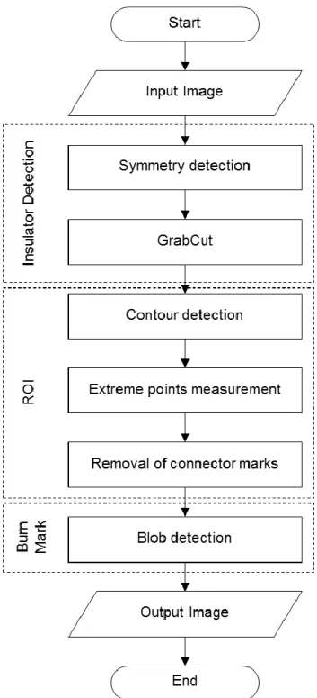
Figure 4.3: Flowchart of Insulator burn mark detection ... 58

Figure 4.4: Nonmaximum suppression ... 60

Figure 4.5: Fast Reflectional Symmetry using edge pixels ‘i’ and ‘j’ ... 61

Figure 4.6: Symmetry detection using Gradient angles ... 62

Figure 4.7: (A) Input Insulator image; (B) Canny edge; (C) Symmetry detection... 63

Figure 4.8: (A) Bounding box w.r.t axis of symmetry; (B) GrabCut output image ... 64

Figure 4.9: (A) Insulator with Symmetrical axis; (B) Elimination of middle section along symmetrical axis ... 65

Figure 4.10: (A) Input Insulator image (without middle section); (B) Detected contours – C1 and C2 ... 65

Figure 4.11: (A) Detected contours; (B) Extreme point detection ... 66

Figure 4.12: (A) Input insulator image; (B) Removal of connector marks; (C) Definition of ROI ... 67

Figure 4.13: Concave (left); Convex hull (right) ... 69

Figure 4.14: Low inertia ratio (left); High inertia ratio (right) ... 69

Figure 4.15: (A) Input image (ROI); (B) Detected burn-mark using blob detection .... 70

Figure 5.1: Flowchart: Symmetry detection ... 72

Figure 5.2: (A) Input Insulator image; (B) GrayScale output image ... 73

Figure 5.3: (A) Input Insulator image; (B) Canny edge; (C) Symmetry detection... 73

Figure 5.4: (A) Input Insulator image; (B) GrabCut output image ... 74

Figure 5.5: Flowchart: GrabCut foreground extraction ... 75

Figure 5.6: Calculation of definite foreground using the axis of symmetry ... 76

Figure 5.7: (A) Input Insulator image; (B) GrabCut output image ... 76

Figure 5.8: (A) Input image (with bounding boxes); (B) GrabCut output image with background patches ... 77

Figure 5.9: Different shades of Insulator (metal part) ... 78

Figure 5.10: Flowchart: Contour detection ... 79

Figure 5.11: (A) GrabCut image; (B) GrabCut output image without the middle part 79 Figure 5.12: (A) WithoutMiddle image; (B) Blurred image ... 80

Figure 5.13: (A) Blurred image; (B) Thresholded image ... 80

Figure 5.14: (A) Thresholed image; (B) Eroded-Dilated image... 81

8

Figure 5.16: (A) Eroded-dilated image; (B) Contour image ... 82

Figure 5.17: (A) Insulator image (at 1m); (B) Insulator image (at 2m) ... 83

Figure 5.18: Probability of burn marks on the insulator ... 83

Figure 5.19: (A) Insulator image (after GrabCut); (B) Insulator image (elimination of connector pixels) ... 84

Figure 5.20: Pixel measurement at 0.5m ... 84

Figure 5.21: Pixel measurement at 1m ... 85

Figure 5.22: Pixel measurement at 1.5m ... 85

Figure 5.23: Pixel measurement at 2m ... 86

Figure 5.24: Marking for extreme points measurement ... 86

Figure 5.25: Flowchart: Defining of ROI ... 91

Figure 5.26: (A) Input GrabCut image; (B) Extreme point measurement ... 92

Figure 5.27: (A) Connector rows of pixel (marked in blue); (B) ROI image ... 93

Figure 5.28: Flowchart: Blob detection algorithm ... 94

Figure 5.29: (A) Input image for blob detection; (B) Blob detection output image ... 96

Figure 6.1: Input images (AD: Capture angle 1; EH: Capture angle 2) ... 98

Figure 6.2: Fault detection algorithm ... 99

Figure 6.3: Algorithm time distribution ... 101

Figure 6.4: (A) Input image; (B) Output image; (C) Calculated distance ... 101

Figure 6.5: Output images (AD: Capture angle 1; EH: Capture angle 2) ... 102

Figure 6.6: Fault detection on Insulator ... 103

9

List of Tables

Table 1.1: Comparison of different HVTL inspection methods ... 13

Table 2.1: Comparison of Image processing tools ... 31

Table 3.1: Overview of different techniques for insulator detection ... 45

Table 3.2: Comparison of foreground extraction methods ... 50

Table 5.1: Readings (Pixel measurement) ... 87

Table 6.1: Insulator detection ... 99

Table 6.2: ROI detection ... 99

Table 6.3: Fault detection ... 99

Table 6.4: Detection rate ... 100

10

List of Abbreviations

BF Brute Force

BGR Blue, Green, Red DoG Difference of Gaussian FCC Flight control computer

FLANN Fast Library for Approximate Nearest Neighbors GLOH Gradient location-orientation histogram

GPS Global Positioning System HSI Hue, Saturation, Intensity HVTL Structured Query Language KNN K-Nearest neighbor

MATLAB Matrix Laboratory MRF Markov Random Fields MRI Magnetic resonance imaging ORB Oriented FAST and rotated BRIEF PCA Principal Component Analysis RANSAC Random sample consensus RGB Red, Green, Blue

ROI Region of interest

SAD Sum of absolute difference SIFT Scale-invariant feature transform SSD Sum of squared difference SURF Speeded up robust features UAV Unmanned aerial vehicle

11

1 Introduction

Over the last few years, the use of Unmanned Aerial Vehicles (UAVs) is growing rapidly in the commercial sector, providing aerial imaging solutions. UAVs equipped with high-resolution cameras act as an excellent investigative and surveillance tool, due to its cheap low power system. The vision for flight control covers a wide range of research areas such as object detection and tracking, position estimation, multivariable nonlinear system modelling, and sensor fusion with inertial navigation and GPS.

In recent years, one such civilian application of UAV is the inspection of High Voltage Transmission Lines (HVTL). Around the world, HVTL is used for transmitting and distributing electricity from generator site to the consumer. Hence, the reliability and performance of these lines are of prime importance. The power lines are constantly affected by rigorous weather conditions and therefore prone to failures. Such failures need to be detected early and fixed immediately.

Figure 1.1: UAV inspecting HVTL [1]

Some of the applications of UAV in this domain include Power Line detection, Insulator fault detection, Detection of snow coverage and swing angles of insulators on HVTL [2], Detection of the insulator dirtiness, and used for maintenance purposes as well. Powerline and Insulator inspection are absolutely necessary for safe operation of power transmission grids. A regular checking is required to detect faults that are caused due to corrosion, mechanical damage or effects of harsh weather conditions. Some methods suggest using a thermal camera for identifying corrosion and damage to electrical wires. Safety and time are the two key factors which make drones handy and attractive in terms of reducing costs and accuracy of work. UAV allows faster defects detection and smooth functioning of high voltage power lines.

12 1.1 Motivation

General motivation:

The inspection of the power lines across the globe is mostly carried out by Humans. Though the reliability is more in this case, it is dangerous and consumes a lot of time. Another way by which HVTL is inspected is by the use of Helicopters [3]. This method is efficient as compared to the conventional one but very expensive.

Figure 1.2: Human HVTL inspection (left) [4]; Inspection by UAV (right) [5]

In order to overcome the drawbacks encountered in the previous techniques, UAV based HVTL inspection method plays an important role. It reduces the inspection cost and time and is safe for the inspection workers. The UAV can also reach to places where it is difficult to reach for humans. Additionally, the power need not be turned off during the inspection period, which is not the case when the inspection is performed by humans. Hence, safety and efficiency increase drastically with this technique.

With the current development, the use of UAVs in HVTL inspection is still human dependent i.e. it is not completely autonomous. Gathering of reliable data and processing it requires a team of well-trained and expert professionals in order to match up with the quality standards. Therefore, as discussed in [6], the best solution is UAV based fully automated HVTL inspection system.

Figure 1.3: HVTL inspection technique development [6]

Monitoring and inspection of insulator and power line incorporate the surrounding objects as well, especially vegetation. There's a regular need to check the vegetation near the power line corridor. Trees, branches or bushes should be regularly trimmed; otherwise, it might lead to electric arcs and danger of fire. For inspection of power line corridors, seven fundamental types of data can be used: Synthetic aperture radar

Human-expert inspection Helicopter inspection UAV inspection UAV automated inspection

13

images, optical satellite images, optical aerial images, thermal images, airborne laser scanner data, land-based mobile mapping data and last but not the least, data from UAV images [7].

Sl.No. Inspection methods Advantages Disadvantages 1. Human-expert inspection Reliable and

accurate

Danger to life, Time consuming 2. Helicopter inspection Time effective and

reliable High cost

3. UAV inspection Safe, Cost and time effective

Tedious to process data manually (5-6

GB)

4. UAV automated inspection

No danger to life, Human intervention

not required, Cost and time effective

Still in development, Accuracy not as

good as human inspection

Table 1.1: Comparison of different HVTL inspection methods

Specific motivation:

The thesis work is part of APOLI [6] project. The objective of this project is to achieve a fully-autonomous HVTL inspection system. A brief insight into the APOLI project is as follows:

14

The UAV has two computers, the Flight control computer (FCC) and Mission Computer (MC). The FCC is the main flight computer and the MC is mission specific. The task of mission computer is to automate inspection with help of FCC and other sensors and actuators. The fully autonomous UAV inspection system has the task to detect the insulator fault and the powerline cable fault. Insulator fault needs to be detected using image processing technique from image/video data. The powerline cable fault can be diagnosed by performing aerial inspection while flying from one tower to another.

The motive to opt for fully autonomous image processing inspection system is mainly because of the following reasons:

1. The data collected (recorded) during the flight path of the UAV based inspection is enormous – around 6 gigabytes. It can be extremely tedious to inspect the video manually. Hence, automated inspection using image processing is the best solution. The final objective is to do the fault detection and inspection real-time.

2. Due to limited availability of memory on the mission computer, machine learning algorithms cannot be incorporated. The whole fault detection system should purely work on image processing algorithms.

3. Due to strong electromagnetic radiation from the HVTL, the conventional orientation and positioning sensors are not working optimally [6].

1.2 Research objectives of the thesis

The objective of the thesis is to develop a post-processing image processing algorithm for fault detection on insulators. ‘Object detection methods’ using image processing is the key research area.

The main objective is listed into multiple sub-objectives which are as follows:  Insulator detection within the image.

 Detection of faults (burn-marks) on the detected insulator. 1.3 Problem Statement

The task of finding burn marks on the insulator had several challenges which were aimed to be solved during the thesis. They are as follows:

15  Insulator detection:

a) Locating the insulator within the image

b) Finding the insulator from a cluttered background c) Extraction of the insulator.

 Elimination of the connector marks: The connector marks on the insulator possess the same characteristics as that of burn-marks; hence this needs to be rejected in the process of the detection.

 Detection of the burn marks on the insulator: It is the final step in the algorithm. Since, the burn-marks don’t have any definite shape, size, and color, some generic algorithm needs to be formulated.

1.4 Overview of the following chapters

The thesis has been structured into several chapters ranging from the basics of image processing to an in-depth evaluation of the insulator. The chapter of introduction was aimed to give an insight of the whole project and where this thesis project fits in. The general motivation for the project and the motivation specific to the thesis is also discussed. The following few paragraphs give a brief description of each chapter and the purpose of it in the thesis work.

 Chapter 2 - Fundamentals of Image processing: This chapter deals with the fundamental literature and background knowledge of image processing and computer vision in general. It also gives a basic understanding of object detection algorithms using feature matching. The last part has an overview of the different image processing tools available and a comparative study has also been conducted.

 Chapter 3 - State of Art: The chapter contains the literature survey and research areas concentrated on topics related to the thesis. It also does a relative study of the pros and cons of the different methods discussed. The first two parts discuss general object detection techniques in depth. The third focus on insulator detection techniques based on different research papers and ideas presented at conferences. The fourth is related to image segmentation methods and the last list the different burn-mark detection algorithms.

 Chapter 4 - Concept: As the name suggests the concept chapter deals with the idea to meet the objective of the thesis. It is the proposed solution for the thesis, listed in a step-wise manner. It also aims at resolving the problems

16

which were listed in the problem statement. From the analysis obtained from the state of art of different techniques, the concept phase selects the one which is the most optimum for this thesis.

 Chapter 5 - Implementation: This chapter shows the implementation of the proposed solution discussed in the concept phase. From insulator detection to burn-mark detection, all steps are listed here. The tools used for implementing these algorithms are also depicted.

 Chapter 6 - Result: The results obtained are discussed and presented in this chapter. An analysis of the different algorithms is done based on the output obtained and the performance is also calculated. It checks for the execution time of the algorithm as well.

 Chapter 7 - Conclusion and future scope: This final chapter discusses the conclusion of the thesis work and the future scope for the upcoming work based on the results obtained as part of this thesis.

Summary of the chapter:

This chapter gives an introduction to the thesis work on insulator fault detection. The importance and application of the project against other conventional methods are discussed and compared based on the pros and cons. It aims to explain the general and specific motivation of the project work, and also discusses the research objectives and the problem statements in a broader sense. The last sub-heading gives a brief overview of the chapters which are to be discussed in detail further in the report.

17

2 Fundamentals of Image Processing

The process of modifying the properties of an image by performing some modifications or alterations by using different functions is termed as Image processing. Modern generation computers with high computing power, digital image processing has several benefits over analog image processing. It permits a wide range of algorithms that can be applied to the input image. The problems related to noise can be avoided by using different types of filtering operations.

The important terms along with their description are as follows:  Image Processing

 Image Analysis  Image Understanding

Some applications include Image stitching, video surveillance, Optical character recognition, Object recognition, Face recognition. It is widely used in almost all domains which include Medical science, in the field Robotics and in autonomous cars as well.

2.1.1 Properties of an Image

An image is a 2D function f(x, y), where (x, y) represent the spatial coordinates and the value of ‘f’ is proportional to the intensity levels and brightness of the image at that point. A digital image is obtained by sampling and discretization in spatial plane and in brightness. The components of such a digital array are referred to as pixels.

18

Each pixel is a measure of the brightness (intensity of light or luminance) that falls on an area of a sensor. An image becomes a matrix of size width * height (e.g. 1024x768), where each element is the pixel brightness (typically an integer between 0 - black - and 255 - white). Color may add a third dimension (RGB components).

Figure 2.2: Pixel information (Gray-scale Image)

Any Image has either of the following color representation [8]:

 Binary Image - Only two colors are present in the image (0-black, 1- white)  Grayscale Image – Represents the information of intensity of light in the image

and not the color. The pixel (gray value) has 256 different shades ranging from Black (total absence of light-0) to White (total presence of light-1).

 True color - Represents natural color images. The popular color spaces are RGB (Red, Green, Blue), CMYK (Cyan, Magenta, Yellow, Black).

Following are the popular image file formats [8]:

 JPG or JPEG (Joint Photographic Experts Group) - Supports color depth of 24 bits (3 color channels of 8 bits each).

 GIF (Graphic Interchange Format) - Supports color depth of 8 bits.

 PNG (Portable Network Graphics) - Supports color depth of 48 bits (3 color channels of 16 bits each).

 TIFF (Tagged Image File Format) - Supports color depth of 48 bits (3 color channels of 16 bits each).

19 2.1.2 Histogram Equalization

The contrast of an image defines the range of brightness or color value taken by all its pixels. This can be visualized by plotting a histogram of pixel intensities.

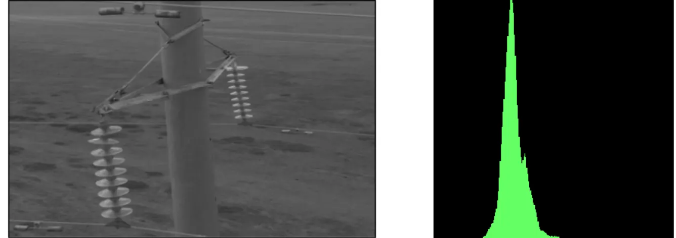
Figure 2.3: Insulator image (in gray scale) before histogram equalization

It can be observed from Figure 2.3 that the pixel intensities are concentrated around a region, i.e. it doesn’t occupy the entire range of pixels from 0 to 255.

Figure 2.4: Insulator image (in gray scale) after histogram equalization

Histogram equalization flattens the distribution of pixel densities so that the whole range of pixels is occupied. This improves the contrast of the image. It doesn’t work well on images with high contrast images, which have a lot of dark/white pixels but nothing in the middle. As it can be visualized from the Figure 2.4 that the entire range of pixel value is occupied [9].

There are a few points which should be considered before applying Histogram Equalization. It can amplify noise in dark areas and can flatten the range in the bright area.

20

2.1.3 Blurring or Smoothening of Image using filters

Almost all images are affected by some kind of Noise. Noise can be interpreted as the disturbances in the intensity of an image. The first and the foremost step in Image analysis is to filter out the noise. Filters are mainly divided into two types: Edge filters are used for detection of edges and Smoothing/Blurring filers are essential for removing of High-frequency Noise (Low pass filter) [10].

Smoothing is defined as the process to remove high-frequency noise from an image. One of the most widely used blurring filters is the Gaussian filter.

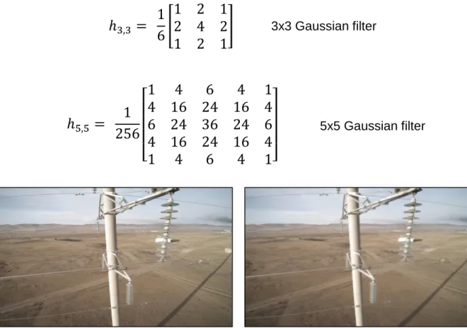
Figure 2.5: Source image (left); blurred (Gaussian- 5x5 kernel) image (right)

The Gaussian noise in digital images gets acquired during capturing the image. For example, noise can be caused by poor illumination, high temperature and/or during transmission. The spatial filter can be used in order to reduce Gaussian noise. Commonly used spatial filtering techniques include median filtering, Gaussian blurring/smoothing and mean filtering.

𝑓(𝑥, 𝑦) = 1 2𝜋𝜎2𝑒 (−𝑥2_2𝜎+ 𝑦₂2) ₍₁₎

ℎ

=

1

6

[

1 2 1

2 4 2

1 2 1

]

ℎ

=

1

256

[

1

4

6

4

1

4 16 24 16 4

6 24 36 24 6

4 16 24 16 4

1

4

6

4

1]

21 2.1.4 Thresholding

Segmentation is the process of separating an image into regions. The property that pixels in a region share is the intensity. Hence, the method to segment those regions by separating the light and dark regions is known as Thresholding.

If g (x, y) is a thresholded version of f (x, y) at some global threshold T,

𝑔(𝑥, 𝑦) = {1 𝑖𝑓 𝑓(𝑥, 𝑦) ≥ 𝑇

0 𝑜𝑡ℎ𝑒𝑟𝑤𝑖𝑠𝑒 (2)

Thresholding only considers the intensity of the pixels and not the relationships between them. This leads to a problem when we try to detect the desired region within an image. Extraneous pixels can be included and pixels within the region which are near the boundaries can be missed. This effect gets worse as the noise gets worse. Therefore, trial and error methodology needs to be applied to get the desired value. It is generally a good practice to apply Gaussian blur before thresholding in order to reduce the noise.

Figure 2.6: Source image (left); binary threshold (right)

Figure 2.6 uses a simple thresholding technique – Binary threshold. This operation involves a global value of threshold applied over the entire image. If a pixel value is greater than the threshold value, that particular pixel value is assigned the threshold value (255, white in this case).

The problem with a global threshold is with the illumination. Variation in illumination across the scene may cause some parts to be darker (in shadows) and some parts to be brighter (in the light). This problem can be rectified by using a locally adaptive threshold algorithm. The algorithm calculates the threshold for small areas or regions in the image [11]. OpenCV (which is used for implementation purpose of the thesis) supports five global thresholding techniques: Threshold Binary, Threshold Binary

22

Inverted, Truncate, Threshold to Zero, and Threshold to Zero Inverted. It also supports adaptive thresholding as well as Otsu’s binarization [12].

Figure 2.7: Source image (left); Adaptive threshold (right)

Figure 2.7 uses locally adaptive threshold technique. The adaptive method used is Gaussian filter and the threshold value is the weighted sum of the neighborhood/near-by pixels. This method is particularly effective when an image has different lighting conditions in different areas.

Otsu Binarization: As discussed above, for global thresholding technique trial and error method needs to be applied to get a good threshold result. But in the case of Otsu binarization method, the threshold value is computed automatically. This method works best with the bimodal image (image with two histogram peaks).

Figure 2.8: Source image (left); Otsu binarization (right)

It can be clearly observed by comparing the results of a simple threshold (Figure 2.6) and Otsu binarization (Figure 2.8). In the latter method, the unwanted white noise and grains are filtered automatically, giving a better result as compared to a simple binary threshold.

2.1.5 Morphological Transformation

The binary images produced after simple thresholding are subjected to grains. These grains are nothing but the noise generated during the conversion into a binary scale.

23

Morphological transformation is a technique by which these grains or noise can be eliminated. This technique can also be applied to grayscale images.

Morphological image processing, a non-linear operation, is used for manipulating the shape or feature in an image. It can also be applied to grayscale images such that their absolute pixel values are of minor or no interest. The morphological technique consists of a template called a structuring element. This structuring element checks all the pixels in the image and compares with the neighborhood pixels.

Square 5x5 element Diamond-shaped 5x5 element Cross-shaped 5x5 element Square 3x3 element

Figure 2.9: Example of structuring elements [13]

Structuring element is a small matrix of pixels with a value of either zero or one. The dimension of the matrix specifies the size of the structuring element. The shape is determined by the pattern of zeros and ones. Odd-dimension structuring element is generally considered to have one pixel as the origin [13].

Erosion:

In erosion, a pixel element with a value equal to one (true) stays true only if all its neighboring pixels are also true. This operation shrinks/erodes the image. A binary image ‘b’ eroded by a structuring element ‘e’ at every locations (x, y) gives a new binary image ‘f’

𝑓(𝑥, 𝑦) = { 1 𝑖𝑓 ′𝑒′ 𝑓𝑖𝑡𝑠 ′𝑏′

0 𝑜𝑡ℎ𝑒𝑟𝑤𝑖𝑠𝑒 (3)

24

Erosion with small square structuring elements (3x3 or 5x5) shrinks an image by stripping a layer of pixels from both outer and inner boundaries of regions. The small grains (salt and pepper noise) are eliminated and the gaps between different regions become larger. Large structuring elements have a bigger effect on the outcome of erosion. Similar results can be obtained by iteration of smaller structuring elements [13].

Dilation:

In dilation, a pixel element with value zero (false) becomes equal to one (true) if at least one of its neighboring pixels is also true. It amplifies the salt and pepper noise. A binary image ‘b’ diluted by a structuring element ‘e’ at every locations (x, y) gives a new binary image ‘f’

𝑓(𝑥, 𝑦) = { 1 𝑖𝑓 ′𝑒′ ℎ𝑖𝑡𝑠 ′𝑏′

0 𝑜𝑡ℎ𝑒𝑟𝑤𝑖𝑠𝑒 (4)

Figure 2.11: Example of Dilation (3 x 3 square structuring elements) [13]

The gaps between different regions get reduced by dilation. The shape and size of the structuring element influence the result of erosion and dilation. Erosion and dilation operations have the opposite effect but present interesting results when applied one after the other. Opening, which removes salt and pepper noise, is erosion followed by dilation. On the other hand, closing is dilation followed by erosion and it is useful in elimination of small holes in the image.

Opening Closing

25 2.2 Feature detection and matching

Feature detection and matching is an important component in Computer vision applications. Some of the applications include Image stitching, 3D reconstruction, motion tracking, object recognition, robot navigation etc. This section discusses the topics of object recognition which are directly or indirectly referenced in the thesis.

2.2.1 Feature detection

Feature detection refers to the finding of a set of interesting points or features. It defines a region around each point. The features that are first noticed at a specific location of an image are mountain peaks, doorways, building corners, shaped patches of an object. These kinds of features are interest points. This is the stage where each image is searched for locations that are likely to match well with other images [14].

Detection of corners, blob detection falls under Feature detection. Some common algorithms are Harris corner detector, LoG/DoG Blob detector.

Properties of a good feature include:

 Patches with high contrast changes (gradients) are considered as good features.

 A good feature should be invariant to Illumination, scale, and pose.  A good feature is never big.

The simplest way to compute the similarity between two images I0 and I1 at different

locations is to compute the weighted sum of squared differences (WSSD):

𝐸𝑊𝑆𝑆𝐷(𝑢) = ∑𝑤(𝑥𝑖)[𝐼1(𝑥𝑖 + 𝑢) − 𝐼0(𝑥𝑖)]2

𝑖 (5)

w (xi) = 1 in window, 0 outside.

where I0 and I1 are the two images being compared, u = (u, v) is the displacement

vector, w(x) is the window function, and the summation ‘i’ is computed over every pixel in the region [14].

26 2.2.2 Feature description

At this stage, the region around the detected key-point locations is converted into a compact and stable descriptor, which is invariant and that can be matched against other descriptors. Feature descriptor technique takes an input image and outputs the feature vectors. A vector of values, known as descriptor, represents the region of an image around an interesting point or it could be some raw pixels. The merger of an interesting point along with its descriptor is called a local feature. Extraction of the local patch around feature is termed as Feature Extraction. For example, SIFT (Scale-invariant feature transform) is both a feature detector and descriptor. The other commonly known algorithm is SURF (Speeded up robust features), which is a faster version of SIFT. Another descriptor, GLOH (Gradient location-orientation histogram) is a variant of SIFT that uses a log-polar binning structure [14].

SIFT:

The SIFT algorithm proposed by Lowe, solves the image rotation, affine transformation, intensity and viewpoint matching features. The algorithm basically consists of four steps, which are as follows:

1. Estimating scale space extrema using Difference of Gaussian (DoG)

2. Localization of a key point, where the key point candidates are localized. Refinement is done by eliminating the low contrast points.

3. A key point orientation assignment based on the local image gradient.

4. Computation of the local image descriptor using a descriptor generator for each key point based on image gradient magnitude and orientation [15].

SURF:

SURF: SURF algorithm uses a Box filter in place of DoG. Instead of using Gaussian average, squares are used for approximation. This is because convolution with the square is much faster if the integral image is used. Another advantage is it can be done in parallel for different scales. The SURF used Blob detector, which is calculated from the Hessian matrix to find the interest (key) points. Wavelet responses in both horizontal and vertical directions are used by applying Gaussian weights for orientation assignment. SURF uses wavelet responses for feature description. A neighborhood around the key point is selected and divided into sub-regions. For each sub-region, the wavelet responses are taken and represented to get SURF feature descriptor. The sign of Laplacian which is already computed in the

27

detection is used for underlying interest points. Bright blobs on dark backgrounds are distinguished from the sign of Laplacians [16].

ORB:

Oriented FAST and rotated BRIEF is a combination of FAST key point detector and BRIEF descriptor with some changes. In order to detect the key points, it uses FAST. Harris corner measure is then applied to find N top points. FAST is rotation invariant, orientation is not computed. FAST (Features from accelerated segment test) computes the intensity weighted centroid of a region with its corner located at the center. The orientation is further obtained by direction of the vector from the corner point to centroid. The rotation invariance is improved by computing the moments. The performance of the BRIEF descriptor (Binary Robust Independent Elementary Features) is poor if there is an in-plane rotation. In ORB, a rotation matrix is computed using the orientation of patch and then the BRIEF descriptors are steered according to the orientation.

2.2.3 Feature matching

This stage searches for likely matching local features in other images. The easiest way to find all corresponding feature points is to compare all features against all other features in each pair of potentially matching images. Unfortunately, this method is inefficient as it requires a lot of computations.

An optimized solution is a work on an indexing structure, such as a multi-dimensional tree which can rapidly search for features near a given feature. The indexing structures can be made for each image individually (for searching a particular object) or globally for all images, which can be faster as it removes the need to reiterate over all images. For large databases (millions of images) vocabulary trees method [17] can be more efficient.

Multi-dimensional search trees are another widely used class of indexing structures. The most common of these is k-d trees [18], which divide the multidimensional feature space along alternating axis-aligned hyperplanes, choosing the threshold along each axis so as to maximize some criterion, such as the search tree balance. OpenCV options for feature matching are Brute Force (BF) and FLANN.

28 2.2.4 Feature alignment

Due to the fact that two images from a similar scene don't necessarily have the same number of feature-descriptors, it needs to be separated by a rejection process. One of the most common approaches to perform correspondence rejection is to use RANSAC (Random Sample Consensus). This step is important to reject all the outliers [14].

2.3 Image processing tools

There are several tools available to develop image processing software. Selection of proper tool is one of the most important criteria for any image processing task. The algorithm developed on hardware with high computational capacity should be able to analyze with ease and perform smoothly. Tools which are most popular are OpenCV (open source computer vision), MATLAB (matrix laboratory), LEAD tools-image processing, Scikit-image. There are some tools available but are mostly application specific. Adobe Photoshop, for example, is popularly used for image editing. The four tools listed are generic and can be used to develop almost any image processing algorithm. Comparisons of these tools are as follows:

2.3.1 OpenCV

OpenCV, open source computer vision library was initialized as a research project at Intel in 1998. Since 2000, it has been accessible and feasible under the BSD open source license. The library was initially is written in C/C++ and runs under commonly used operating systems such as Linux, Windows and Mac operating system. The library is available for Python, Ruby, Matlab and other languages. The key design parameters for OpenCV are computational efficiency and a strong focus on real-time applications. It is basically a collection of commonly used functions that perform operations related to computer vision. OpenCV has wrappers for Python, Java and other JVM dialect which is to perform Java bytecode, for example, Scala and Clojure. Since most of the app development is done in C++/Java, OpenCV has been ported as an SDK for developers to use and implement it in their apps and make them vision enabled. A new module was added to OpenCV in 2010 that maintains GPU-acceleration. The GPU module covers an important part of the library functions and is still in active progress. It is executed using CUDA. The users can take the benefit from GPU-acceleration without in-depth training in GPU programming. The GPU module is constant with the CPU version of OpenCV, which makes maintenance easy. The raw image data in OpenCV can be accessed by cv::Mat, which is a

29

container for images. The OpenCV library consists of numerous functions and has applications across all domains such as security, camera calibration, robotics, medical imaging and factory inspection. In many applications in the modern era, machine learning is actively used along with computer vision algorithms. Hence, a universally useful Machine Learning Library (MLL) is added to OpenCV. A sub-library which is focused on pattern recognition and clustering is also added [19].

Figure 2.13: OpenCV logo [19]

2.3.2 MATLAB

MATLAB is a programming language, used for mathematical analysis and design of processes using matrix and arrays. It is a desktop application, developed by MathWorks. It supports several functionalities such as data analytics and plotting, data manipulation, algorithm development in image processing and machine learning etc. Interfacing with functions such as C#, C, C++, Java, and Python is possible with Matlab. It comes with an additional package of Simulink, which supports model driven programming and graphical simulations. Symbolic computing is also possible by using an optional MuPAD symbolic engine. Some of the application areas of Matlab include Deep Learning, Computer vision, signal processing, areas of quantitative finance and risk management, robotics and control systems.

Image processing toolbox of Matlab is responsible for computer vision tasks. It provides a complete set of standard image processing algorithms for analysis, visualization, and development. It performs image processing tasks such as segmentation, noise reduction, image enhancement, feature detection and matching. The Image processing toolbox allows automation of common image processing workflows. The visualization apps support image exploration, 3D volumes and videos, contrast adjustment, histogram creation and manipulation of region of interest. Image processing algorithms can be accelerated by running them on multi-core processors and GPUs. It has toolbox functions which supports high level C or C++ code generation for desktop and embedded [20].

30

Figure 2.14: MATLAB logo [20]

2.3.3 Scikit-image

Scikit-image just like OpenCV is an open source image processing library for programming in Python. It supports algorithms for geometric transformation, filtering, color space manipulation, morphology, feature detection, segmentation, analysis, feature detection and some more. It can interoperate with the NumPy and SciPy scientific libraries of Python [21].

Figure 2.15: Scikit-image logo [21]

2.3.4 LEADTOOLS

LEADTOOLS SDK imaging allows tool developers to access powerful image processing algorithms which can be directly used for different applications. It is there for more 25 years in imaging development. Leadtools supports more than 150 image formats and supports image compression, image processing, and image viewers. The programming interfaces and platforms supported by Leadtools are Android, C++, Java, C, .NET- C#, HTML5/JavaScript, VB. The operating systems supported are Android, iOS, Linux [22].

31

Tools Advantages Disadvantages

OpenCV - Supports C, C++, Java, Android, Python - Open Source

Not as interactive as MATLAB MATLAB - User-friendly

- Supports model-driven programming Licensed tool

Scikit-image - Open Source Supports only

Python

LEADTOOLS - Better user interface Licensed tool

Table 2.1: Comparison of Image processing tools

Summary of the chapter:

This chapter briefly discusses the basic understanding and fundamental concepts of Image processing. These concepts are particularly important for the understanding of the thesis work.

The first section deals with the general preprocessing algorithms which are essential for almost any image processing task. Starting with the characteristics of an Image, the sub-point discusses the coordinate system of a 2D image, basic idea of pixels, different color spaces, and the image formats. The Cartesian coordinate system of 2D images has a different representation to that used in mathematics. The following sub-point list down the different preprocessing algorithms. The main purpose of these algorithms is to filter out different kinds of noise from the image.

The second section discusses the feature description and matching algorithms. Further, the section is divided into four sub-points: feature detection, feature description, feature matching and under each sub-point different algorithms are analyzed and compared. The last section lists the different image processing tools available and a table has been prepared based on the pros and cons.

32

3 State of Art

There are different methods for detecting faults in insulators, for example - electro-technical measurements or visual inspection methods are used for examining mechanical damage and flashover marks, but not much research has been done in order to detect burn marks in insulators. Section 3.3 discusses the various methods of detecting different kinds of faults in insulators. In section 3.4, a comparative study has been on the various foreground extraction techniques. Section 3.5 discusses the methods to detect burn/black marks on images using different Blob detection algorithms. References have been taken from the medical image processing domain in order to detect the black spots.

3.1 Object detection using Template Matching

Template matching technique uses a predefined template to search for a match in an image. It uses pixel by pixel match of the template image within the input image. Sophisticated template matching techniques can detect multiple presence of the template within the image irrespective of the orientation and scale.

Template matching is one of the common methods used for object localization because of its user friendliness. The major drawback is it requires high computational power to perform pixel by pixel search operation. The size of the template is directly proportional to the amount of time required for processing.

The basic template matching algorithm involves in calculating at each position of the image under examination a distortion function that measures the degree of similarity between the template and the image. The maximum correlation or the minimum distortion is used to locate the template into the target image [23]. The similarity between two regions in an image is given by the correlation value. For two regions to correlate, it isn’t mandatory that all pixel values should exactly match but in general behavior [24].

The typical distortion measures are the Sum of Absolute Difference (SAD) and the Sum of Squared Differences (SSD) [25].

SAD: 𝑐(𝑥, 𝑦) = ∑. 𝑊 𝑘=0 ∑|𝑓(𝑥 + 𝑘, 𝑦 + 𝑙) − 𝑡(𝑘, 𝑙)| 𝐻 𝑘=0 (6)

33 SSD: 𝑐(𝑥, 𝑦) = ∑. 𝑊 𝑘=0 ∑[𝑓(𝑥 + 𝑘, 𝑦 + 𝑙) − 𝑡(𝑘, 𝑙)]2 𝐻 𝑘=0 (7)

For a given image ‘g’, we want to match the template image ‘f’. Over a given area ‘A’ and an input image ‘g’, the technique of squared difference is generally used to calculate the degree of similarity between the template ‘f’ and ‘g’.

Figure 3.1: Template Matching (f<g) [23]

The maximum value of the squared difference gives the measure of similarity. The equation of sum of squared difference between template f and image g over region A is given by (2D): ∑ . . 𝑖,𝑗∈𝐴 ∑(𝑓(𝑖, 𝑗) − 𝑔(𝑖, 𝑗))2 . . (8)

Expanding the equation (8), we get:

∬ (𝑓 − 𝑔)2= ∬ (𝑓)2+ ∬ (𝑔)2− ∬ (2𝑓𝑔) 𝐴 𝐴 𝐴 𝐴 𝐴 𝐴 𝐴 𝐴 (9)

In (9) the term ∬(𝑓)2 and ∬(𝑔)2 is fixed and constant. The remaining term ∬(2𝑓𝑔)

gives the measure of similarity between template f and image g.

However, normalized cross-correlation method is robust and one of the most commonly used templates matching criteria when accuracy becomes important [26]. Especially in two-dimensional cases, template matching has many applications in object tracking, medical image processing, image compression and other computer vision applications [24]. As part of this thesis, a template matching technique has been researched upon using OpenCV library. The idea was to search for the burn

34

mark (considering that as the template image) in the insulator image (original image). The result is shown below:

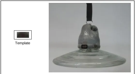
Figure 3.2: Template (Image enclosed in box) (left); Insulator Image (right)

Normed Cross-correlation method has been used (CV_TM_CCORR_NORMED). The function available in OpenCV for template matching is matchTemplate(). It can be clearly observed from Figure 3.2 shows that the template image is able to search for a burn mark in the Insulator image but not all the marks are getting detected. This is due to fact that template matching performs a pixel by pixel comparison; therefore, it fails on other burn marks in the same image or in a different one.

Moreover, this naïve template matching technique is not robust to change in scale or in the rotation. Advanced template matching techniques such as Grayscale based matching and Edge-based matching are invariant to both scale and rotation invariant and more efficient as well but still have some significant limitations and drawbacks. To overcome the cons of template matching method, an efficient way to identify and detect key points is by extracting the local key-point descriptors and applying feature matching technique. More about this is discussed in section 3.2.

3.2 Object detection using Feature detection and matching

As discussed briefly in section 2.2, feature detection and matching technique are used actively for object recognition. Feature detection and matching technique have been used for Insulator detection as described in [27]. SIFT is the feature detector and descriptor used in this method. The method used and the steps implemented in [27] are as follows:

35 1. Algorithm for Image feature detection:

Step 1: Conversion of the image into grayscale. Step 2: Implementation of scale-space construction.

Step 3: Estimation of DoG on images after generation of scale space. Step 4: Finding key-points using DoG scale.

Step 5: Elimination of contrast and edges.

Step 6: Estimation of orientation for each detected key-point. Step 7: Drawing of key-points on the input image.

2. Algorithm for Image descriptor:

Step 1: Sampling of orientation and gradient magnitude around the key points. Step 2: Overlaying of Gaussian window on the samples.

Step 3: Accumulation of samples on the histogram of orientation. Step 4: Achieving the descriptor output.

(A) (B)

Figure 3.3: (A): Insulator template image; (B) Key-points on input image [27]

Figure 3.3 shows the template insulator image and the Input image. Applying the above feature detection and image descriptor algorithms, the corresponding points/feature are detected on the template and the input image. Once the key-features are extracted from both the images, the next step is matching the key-features using some Feature matching algorithm. Flann or Brute Force feature matcher is the most commonly used algorithms.

Brute Force (BF) feature matcher is used for Image Matching. K-nearest neighbor algorithm is applied to compare the key-points in the image and template image. Thresholding is then performed and the matching key-points are selected.

36

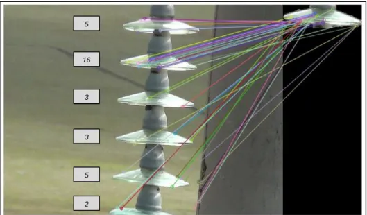
Figure 3.4: Key-points matching with the template image

Figure 3.4 shows the matching of key points between the template image and the insulator image. The digits on the left hand side display the number of good matches with that of the template image. Since the template image is taken as the second insulator; the good matches have maximum value in that case. Further, the RANSAC algorithm is applied for feature alignment.

Figure 3.5: Feature alignment using RANSAC [27]

In order to clarify further Insulator detection using feature detection and matching technique, SURF algorithm has also been tried as part of this thesis work.

16 5 3 3 5 2

37

The feature matcher used is FLANN. The steps are briefly discussed below: Step 1: Conversion of both the template and input images into grayscale. Step 2: Detection of key-points and extraction of descriptors using SURF. Step 3: Descriptor vectors matching using FLANN matcher.

Step 4: Calculation of Max and Min distances between key points. Step 5: Filtering of good matches (distance < 3 times the min distance). Step 6: Calculation of Homography using RANSAC to reject bad matches.

Figure 3.6: Feature detection and matching using SURF

Figure 3.6 depicts a similar result to that of SIFT. The left part is the template insulator, having different scale and color intensity. The features in the input image are getting matched with the template image and Insulators are also detected but the result is not so convincing.

Though feature detection and matching technique is a powerful tool to detect objects, the performance dampens when the features are not distinct. In the case of Insulators, which doesn’t possess a distinct feature, detection becomes a challenge. As described in [27], different template images are taken for different illumination conditions and in most cases, the insulators are detected partially. This happens because the SIFT feature detector detects some false key-points. It generally points to a region somewhere near the insulator but not able to say the exact position. For the task of this thesis, getting the exact location of the insulator is a necessity because the burn marks need to be identified on the Insulator and not somewhere in the background or region close to it. The insulator is detected properly and not partially in Figure 3.5 because the template image is taken as one of the insulators from the same image.

38 3.3 Insulator detection techniques 3.3.1 Detection of snow on Insulator caps.

There is no full-proof inspection technique which has the ability to detect all possible faults [28]. While capturing the insulator image, the lighting conditions and background may change abruptly (e.g. sunshine, cloudy, foggy, drizzle, raining, and snow; moving clouds, airplanes, birds). Therefore, in order to detect the insulator as discussed in [2], the first and foremost challenge is to detect the insulator from the background.

Figure 3.7: Insulator image in different outdoor scenarios [2]

From left to right as shown in Figure 3.7 (i) sunny with clear sky; (ii) insulator with reflections from sunlight; (iii)-(v) non-uniform background due to clouds; (vi)-(viii) blurred images due to the fog; (viii)-(x) dark and night images; (xi) snow on shells; (xii) ice on shells

A region of Interest (ROI) containing the insulator is extracted first in order to limit the computation. For extraction of ROI, image analysis methods such as segmentation, corner detection, histograms often require tuning parameters that do not work well for a broad range of scenarios. The method used in [2] uses a priori information (pre-stored template) and cross-correlation. The template image, containing the outer boundaries of the insulator from an ideal image is matched with the original image to determine the ROI.

After extraction of the ROI, detection and further analysis of snow coverage is performed. In order to detect accurately, prior information is studied and therefore concluded that an insulator is a rigid object, with its size, edges and outer boundaries are fixed. Hence, any changes to this are caused due to external factors such as snow. The second conclusion states that there exists some difference in intensity between the snow and the insulator/background. The third is the intensity difference between snow and insulator shell, which results in extra edge curves on the top half of the insulator shell. Based on these observations, it can be assumed that snow gets accumulated only at the top or along the side of the insulator’s shell.

39

Figure 3.8: Different snow scenarios on insulator [2]

The Fig(No.) above shows the different snow scenarios: (i)(ii) snow; (iii) melting of snow; (iv)(v) Rim frost; (vi) night image with no wind; (vii) night image with a wind speed >10.4m/sec.

The methodology used in [2] to detect snow on insulator shell is as follows:

1. Detecting extra regions: The snow generates extra edges, which is compared and subtracted out from the edges under ideal condition (without snow). The edge detector is applied followed by a median filter to reduce noise.

2. Finding extra regions on top of the shells: Taking prior information on the dimension of the ellipse shell as standard, the extra regions on shells formed due to snow, can be found and analyzed further.

3. Tightening the width of ROI: The ROI is narrowed down by tightening the width defined by two parallel lines touching the outer sides of shells.

4. Intensity comparison: To compare the range of intensity values in the extra regions, region analysis is performed with those of the shell and that of the background.

5. Computation of snow coverage: Once the region of snow is determined, narrow-width vertical bar parallel to the vertical center axis of the insulator is placed and moved from left to right under the sweeping bar. The area under the sweeping bar is the detected snow region, which is then compared with the total length of insulator shells under analysis, resulting in the percentage of snow coverage.

40 3.3.2 Recognition of tempered glass insulator

In paper [3], a method to recognize tempered glass insulator based on intensity in HSI modal from the airborne image by helicopter has been proposed. The stepwise method is as follows:

1. RGB to HSI

The intensity of the tempered glass in the insulator image is higher as compared to the other regions in the image, this is the key factor taken into consideration for detection. First, the image is converted from RGB to HSI color format as shown in Figure 3.9.

Figure 3.9: Insulator image in RGB (left); HSI (right) [3]

2. Binary and Morphological erosion for noise reduction

The HSI converted image is then thresholded using a Binary threshold filter. It can be observed from Figure 3.10 that the insulator part has a higher gray level as compared to other objects in the image such grass, trees etc. Morphological erosion process is further done to remove the noise.

Figure 3.10: Binary thresholded image (left); eroded image (right) [3]

3. Extraction of connected components

The connected component method is used to extract the insulators from the Binary image. Figure 3.11 shows the graph of the connected area. X-coordinate

41

marks the connected components and Y-coordinate represents the amplitude of each connected component. The distribution of insulators can be clearly depicted as they are clustered together and of the same intensity.

Figure 3.11: Analysis of connected area [3]

3.3.3 Insulator detection using regular texture pattern

The research work as published in a paper [29] states that the intelligent diagnosis of the insulator can be achieved using computer vision technology, which refers to insulator detection, image segmentation and fault identification from aerial images. Target detection technique, which is widely for analysis of complicated scenes in intelligent systems, is used for accurate detection of the insulator. The detection is automatic and is based on the geometry and statistical properties of the target. When an image is captured from different angles or distance, the appearance is different but the target itself doesn't change. Humans are gifted with the power of extracting invariant information but for computers, they should extract the invariant features to recognize patterns, and then detect and identify targets.

Regular texture pattern characteristics of insulators are considered to detect the insulators together. The near-regular textures are not a random collection of texture elements but exhibit specific topological, statistical and geometric relations. Hence, "deformed lattice detection" [30] theory has been applied for detection of texture pattern recognition. The steps are as follows:

1. The low level visual invariant features are analyzed in order to generate the high-level insulator lattice model.

42

2. Lattice finding is performed by using an MRF model and multiple insulators are searched.

3. The insulator targets are located by extracting a minimum bounding rectangle.

3.3.4 Insulator detection using texture feature sequence

In this method [31], a combination of Morphology, Hough transform line detection and statistic texture feature are applied for detection of insulator fault.

In order to eliminate some noises during image capturing, it is first preprocessed. The preprocessing is steps include conversion of RGB to Gray, Image enhancement, and morphological transformation. Hough transform line detection technique is then used to correct and analyze the insulator's tilt, which affects the insulator fault detection. The insulator tilt is caused by the instability of the helicopter and the image shooting angle. Then, the processed insulator image is divided into ten parts and each of the ten parts is separated into seven texture values. A 7x10 matrix is formed, in which the seven rows, defined as a sequence, represent the seven texture features and the ten columns represent the ten parts.

Out of the seven feature sequence curves, three sequence curves are selected because they are active. The result is achieved by doing an analytical study. A fault feature named as CMV curve is one out of the three features. Insulator fault is detected by this CMV curve. The biggest value of the CMV curve locates the position of the fault.

43

3.3.5 Insulator fault detection using gradient based descriptor.

This method [32] presents an approach to detect insulators in aerial images and performs an automatic analysis for fault detection. The objective is to check the glass part of the insulator for possible faults or damages. The detection technique is based on discriminative training of local gradient-based descriptors and voting scheme for localization. Further, automatic extraction of insulator cap is performed.

The first step is to detect the insulator and based on that fault analysis is performed. Insulators are weakly textured objects surrounded by a cluttered background, making detection difficult. On the other hand, insulators have a fixed and rigid form with repetitive geometric structure and a definite elliptical shape. These properties are important for the detection and can be further exploited.

For detection purpose, a part based model with a circular descriptor is used, where each insulator glass cap is one part of the model. The model geometry is the major axis, where all insulator caps belonging to the insulator must lie near other detected caps and close to each other. DoG filter is used for the detection of key-points in the image and a square image patch is extracted around the key-point corresponding to the size of the key-point. From the patch, circular GLOH like descriptor is calculated. The circular GLOH is similar to the GLOH descriptor.

The descriptor used is based on image gradients and are derived by the Scharr operator. As compared to other gradient operators, this operator exhibits better rotational invariance and is beneficiary as the caps are circular. For scale invariance, the spatial support is enlarged according to the size of the key-point. Principle component analysis (PCA) is used to reduce the dimensionality of the descriptor for speedup but without loss of classification performance [33]. K-Nearest neighbor (KNN) classifier is trained with descriptors of detected DoG key-points from the training set. For recognition, the classifier is then queried with the descriptors of the detected key-points in order to distinguish between the background clutter and insulator caps.

The bounding boxes for the insulators are then determined from the classified key-points. The grouping of the key-points is done by their scale and an adapted RANSAC approach is applied on all the key points of each scale to robustly fit the insulator model to the detected key-points. Estimation of the fundamental period of