How cyclical do cyclically-adjusted balances remain?
An EU study
*
ENRIQUE ALBEROLA JOSÉ M. GONZÁLEZ MÍNGUEZ PABLO HERNÁNDEZ DE COS JOSÉ M. MARQUÉS
Banco de España
Recibido:Octubre, 2002 Aceptado:Mayo, 2003
Abstract
Observed budget balances are an imperfect indicator of the fiscal policy stance, because fluctuations in economic ac-tivity induce automatic changes in the balance, hence the use of cyclically-adjusted balances (CAB). However, this paper shows that CABs (as measured through one of the two methods currently used by the Commission) tend to be systematically overestimated during downturns and underestimated during expansions. The dominant source of this distortion arises from the filtering of revenues deemed to be cyclical, possibly signalling a problem with the compu-tation of elasticities. The effect of the items which are assumed not to move with the cycle is non significant, but this overall result conceals offseting effects: public investment turns to be significantly procyclical and interest payments and transfers to firms are countercyclical.
Keywords:cyclically adjusted balances, fiscal policy, EU. JEL Classification:H6, E6.
1.
Introduction
Observed budget balances are an imperfect indicator of the fiscal policy stance. Fluctua-tions in economic activity give rise to automatic changes in various components of public expenditures and receipts, so that the budgetary position will worsen under adverse
eco-nomic conditions and vice versa. This prevents anya prioriassessment about whether an
im-provement in the actual government balance during an expansion can be ascribed to the fa-vourable economic conditions, to a genuine consolidation course followed by fiscal authorities or even to the economic expansion outweighing a discretional relaxation in
bud-* We are grateful for helpful comments received from participants in presentations held at the Bank of Spain, the Meeting of the Swedish Committee on Stabilization Policy in EMU (Stockholm) and the Congress of the International Economic Association (Lisbon). The opinions presented here reflect the authors’ views and not the institution where the authors are affiliated.
getary policy. Conversely, and by the same token, a deterioration in the observed balance at a time of decelerating economic activity might be consistenta priorieither with the negative impact of the cycle on the government accounts, with an expansionary stance of fiscal policy in order to counteract weak economic activity or even with an orientation of fiscal policy which is restrictive but not enough in order to overcome the influence of the cycle on ob-served balances.
Thus, the need for instruments to distinguish between the respective impacts of both the economic cycle and discretionary actions on observed balances. If anything, this necessity has been reinforced within the EU boundaries by the multilateral surveillance procedures in force since the Stability and Growth Pact (SGP) became effective. The SGP provision of achieving an outcome which is «close to balance or in surplus» (CTBS) over the medium term might well be interpreted as a requirement to approximately balance either observed budget outcomes on average over the full length of the business cycle or, alternatively, cycli-cally-adjusted balances (CABs) every period. Indeed, CABs are conceptually better suited than observed balances for their use as early warning signals of budgetary positions entailing the risk of breaching the SGP rules under less favourable economic conditions. Thus, com-pliance of a given fiscal position with the CTBS provision is likely to be better assessed through the use of measures of CABs, whose changes should genuinely capture shifts in the fiscal stance1.
However, while being conceptually appealing, the notion of CABs is not easily trans-lated into practice. This is attested by the fact that CAB calculations (usually performed, among other institutions, by international organisations) often yield different results accord-ing to the methodology applied. Generally speakaccord-ing, the gap between the CAB concept and its practical implementation is bridged through two consecutive steps which involve, respec-tively, (i) the calculation of some measure of the departure of the actual position of the econ-omy from a theoretical environment characterized by neutral cyclical conditions and (ii) the estimation of the impact of that departure on observed budgetary outcomes.
The motivation behind this paper is to explore how well the CAB concept is put into practice, by examining whether estimated CABs conform to the theoretical objective of de-vising a measure of budgetary results truly deprived of any systematic cyclical pattern. To do so, the results stemming from a particular methodology have been selected. In particular, we have chosen one of the two methods that the European Commission will use for the assess-ment of Stability and Convergence programmes from Autumn 2002 onwards (to which we will refer from now on as «the European Commission method»). Focusing on a particular method implies that the paper does not try to assess the superiority of alternative procedures for calculating CABs. Moreover, for the European Commission method, the suitability of the way to broach the first step of the computation is not scrutinized, but rather taken as given, however questionable it might be.
Thus the focus falls upon certain aspects of the second step of the calculations. In fact, commonly used procedures for calculating the budget balances that would be observed under neutral cyclical conditions take as a starting point ana prioriassumption about the various
budgetary categories of expenditures and receipts which are sensitive to the business cycle and those which are not. This distinction, often unchallenged, is grounded on the legislative provisions that make those budget items react automatically to economic conditions. How-ever, it might well be possible that other items which are assumed not to be cycle-sensitive on the grounds that no such an automatic link to economic conditions exists, may in practice be cycle-sensitive. This would not be so because of the existence of any provision enshrined in law, but rather because of a systematic discretionary reaction on the side of fiscal authori-ties. This is one of the two main issues which are brought to the limelight in the paper, the second one being the possibility that, for cycle-sensitive items, the decomposition between their cyclical and cyclically filtered subcomponents is not done in a fully appropriate way. Consequently, the main aim of this paper is to explore whether these two possible sources of misadjustment are relevant and, if so, to quantify their impact on calculated CABs.
The paper intends neither to provide precise proposals for improvement on commonly used measures nor to make a strong case for the inclusion of assumed purely structural items in the calculations. Rather, it can be seen as an attempt to point out to some problems in the calculations which have been so far overlooked and to open new avenues for further re-search.
The analysis is performed mainly within a panel data framework, as advised by the char-acteristics of the available sample, which consists of a relatively short time series for as many as fourteen countries (all EU member states but Luxembourg). This is complemented by a less in-depth analysis of the time series and cross section dimensions of the sample, which attempts to capture, respectively, possible intertemporal and individual country changes in the behaviour of the structural components of the various budgetary items. The panel results reveal mainly that those revenue items which are cyclically-adjusted by the Eu-ropean Commission retain a cyclical behaviour even after adjustment (namely, a countercyclical one)2. Besides, among those items which in the Commission method are as-sumed not to move with the cycle, the procyclical behaviour of public investment and the countercyclical one of interest payments do stand out.
The paper is organized as follows. Section 2 presents the budgetary categories building the non-financial general government accounts, stressing which particular items are typically subject to cyclical adjustment in practical calculations of CABs and which are not. Next, in section 3, the European Commission methodology for calculating CABs is briefly described, while section 4 performs a preliminary exploration of the possibility that calculated CABs are in fact not orthogonal to the business cycle. Section 5 presents a simple methodology which can be used in order to check whether both the calculated cyclically filtered compo-nents and the assumed purely structural compocompo-nents are in fact uncorrelated with the cycle, as well as providing a quantification of the extent to which the CAB responds, on account of each item, to changes in the output gap. The results of applying our methodology are shown in section 6. As already stated, this is initially performed in a panel data framework, followed by a more detailed time and country analysis. Main conclusions are summarised in the final section of the paper.
2.
Structure of public accounts
The non-financial accounts of the general government record the non-financial transac-tions in which its units (i.e. the central government, regional and local governments and the social security funds) engage. These transactions are classified in national accounts under various categories of receipts and expenditures, with the difference between their respective totals providing the general government budget balance. Obviously, even if such classifica-tions are performed on the basis of the economic nature of the underlying transacclassifica-tions, some conventions are required. With the move from the old version of the European System of Ac-counts (ESA-79) to the new version (ESA-95), the categorization of transactions in the gen-eral government accounts has undergone major changes. However, even if ESA-95 provides a classification which in some respects is possibly better suited to the purpose of this paper, ESA-79 has been retained here as the accounting benchmark, given the unavailability under ESA-95 of the long dated time series which are required3.
The calculation of cyclically-adjusted budget balances is described in figure 1. Typically, it involves, as a first step, drawing a dividing line between the receipt and expen-diture items which are assumed to be sensitive to the cycle and those which are not. Next, an attempt is made to deprive cycle-sensitive items of cyclical influences, with the aid of some statistical procedure. Then, the cyclically-adjusted or structural balance is computed by add-ing these calculated cyclically-adjusted components of the cyclical items and the observed items which have been assumed not to be cycle-sensitive (each single item being entered with the appropriate sign, i.e. positive —negative— when dealing with a receipt —expendi-ture— heading). Chart 1 presents, on its left-hand side, the list of revenue and expenditure items which make up the general government non-financial accounts4. Cycle-sensitive items (shown in italics in the left-hand side of figure 1) are decomposed in the right-hand side into their cyclical and cyclically-adjusted components, while items of a cycle-insensi-tive nature (denoted as purely structural items) are entered into the calculation of the CAB without any correction.
On the revenue side, there are four different items which are usually assumed to display a cyclical pattern and thus are subject to cyclical adjustment. These are:indirect taxes, direct taxes on households, direct taxes on firmsandsocial security contributions.All of these cat-egories of revenue are characterised by being linked, via legal provisions, to some macroeco-nomic aggregate displaying a cyclical pattern.
Among expenditure items, onlyunemployment benefit payments(UBP) are usually as-sumed to display a cyclical pattern insofar as the number of unemployed people, and conse-quently total unemployment payments, will decrease (increase) in the upper (lower) part of the business cycle. It is worth noting at this stage that UBP are generally not singled out in national accounts. On the contrary, they appear included within the more general category of current transfers to households.
The remaining budgetary items (either on the revenue or on the expenditure side of the budget) are usually not subject to cyclical adjustment on thea priorigood grounds that no le-gal provision establishes an automatic link between these categories and the business cycle.
On the revenue side, these are the current resources not included in any of the above mentioned categories (labeled asother current receipts)5. Nearly all expenditure items are usually assumed not to display any cyclical pattern. These include, among current expendi-ture, government consumption, current transfers(to households and to enterprises),net cur-rent transfers to the rest of the worldandinterest payments.Among capital expenditure two items arise, namely,final capital expenditureandnet capital transfers paid.
3.
Computation of structural deficits
Currently, various methods are proposed in the literature to separate the budget balance into its structural and cyclical components. The standard methods involve two main steps. First, they estimate the cyclical fluctuations (output gaps) by subtracting the potential or trend output from actual output and expressing the difference as a percentage of the former. Second, they estimate the cyclical component of the budgetary balance through the applica-tion of fiscal elasticities. Finally, this cyclical component is deducted from the actual budget
Figure 1. Decomposition of the cyclically-adjusted balance
CYCLICAL COMPONENTS
Revenues Indirect taxes
Direct taxes on households Direct taxes on firms Social Security contributions
Other current receipts
Expenditures Unemployment benefits Public consumption Public investment Interest payments Transfers to firms Transfers to households Transfers to rest ofworld Net capital transfers paid Other capital expenditures
CYCLICALLY
BALANCE -ADJUSTED Cyc. adj revenues
Cyc. adjunempl. ben.
Public consumption Public investment Interest payments Transfers to firms Transfers to households Other revenues Other expenditures CYCLICALLY-ADJUSTED COMPONENTS PURELY STRUCTURAL ITEMS
3 levelrd 2ndlevel 1 levelst
ECONOMETRIC ANALYSIS CATEGORIES STRUCTURAL-CYCLICAL DECOMPOSITION
balance to derive the structural (cyclically-adjusted) component. This is the approach used by most of the international organizations, including the OECD, the IMF and the European Commission (EC). The main difference among the indicators produced by these institutions involves the calculation of the output gap, which is estimated via a smoothing technique in the single method used by the EC until recently or through a production function in the case of the OECD and the IMF [Giornoet al.(1995); Jaeger (1993)] and also in a new method de-vised by the EC itself.
In this section, we describe in detail the method applied by the EC to calculate cycli-cally-adjusted balances (CABs).
3.1.
Estimates of trend output
The European Commission (1995) calculates trend output applying the Hodrick-Prescott filter to the real GDP series6. This method is based on the minimisation of the square of the deviations in the actual output around the trend output subject to a restriction on the change in the trend growth rate:
subject to
[1]
which can be rewritten:
[2]
whereyis the logarithm of actual real GDP,y*is the logarithm of real trend GDP,kis a small number, chosen arbitrarily andlis the Lagrange multiplier.
The estimate of the output gap (GAP) is obtained taking the quotient of the difference between GDP and trend output, and this latter variable:
[3] * 2 1 min (T t t) t y y =
-å
* * * * ( ) ( ) é ù £ ë ûå
T -1 2 t+1 t t t -1 t=2 - - - k y y y y 1 * 2 *1 * * *1 2 1 2 min (T t t) T (( t t) ( t t )) t t y y - y+ y y y -= - + l= - --å
å
* * Y Y GAP Y -=3.2.
Computing CABs
Calculating cyclically-adjusted balances once the output gap measure has been esti-mated involves, in the case of the EC methodology, to single out the budgetary items which are assumed to display a cyclical pattern as described in the previous section of this paper. Next, the part of these cycle-sensitive items which is attributable to the economy's cyclical position (as approximated by the output gap) is obtained. Calculated cyclical components of cycle-sensitive public revenue and spending items are based on the estimates of their elastic-ities to the output gap.
The cyclical component of public revenue (CR—in % points of GDP—) is obtained by
multiplying the elasticity of revenue in relation to GDP (eR) by the average revenue/GDP
ra-tio [(R/Y)t], and by the output gap (GAPt)7:
[4]
The revenue elasticity applied by the EC is calculated as an average of the respective elasticities of each of the revenue groups considered, weighted by the relative proportion of each of these categories to total revenue. The Commission takes as given the elasticities cal-culated by the OECD for each of the four revenue categories considered:corporate income tax, personal income tax, social security contributionsandindirect tax.As it has been ex-plained in section II, no cyclical adjustment is made neither to the itemother current revenue
nor to the itemcapital revenue8. Therefore the revenue elasticity is:
[5]
whereeRt,eCt,ePt,eSSt,eItare the elasticities of total revenue, corporate taxes, personal
inco-me taxes, social security contributions and indirect taxes; andRCt/R, RPt/R, RSSt/R, RIt/R
are the shares of each component in total revenue (R)9.
The output elasticity of each of these revenue categories is calculated by the OECD [Giornoet al.(1995)]10as follows:
The elasticities of income tax and social security contributions are obtained from the ratio between the values of the average and marginal rates of these levies. However, this ratio gives the elasticities of income tax and social security contributions in relation to gross nominal wages. To obtain the elasticity in relation to GDP, the foregoing elasticity is adjusted in terms of the re-sponse that employment and wages show in relation to fluctuations in real output.
The elasticity of corporate income tax is calculated on the basis of a simple regression of the revenue for this tax over output at current prices11. Finally, the elasticity of indirect tax
revenues is considered to be one.
As to the cyclical component of public spending and as it has been explained in section II, all but one particular item are usually assumed not to move with the cycle. In particular, the EC only considers unemployment benefits spending to exhibit a cyclical behaviour.
Cal-( / ) · = e Rt t R t C R Y GAP Ct Pt SSt It Rt RR Ct RR Pt RR SSt RR It e = e + e + e + e
culation of the elasticity of this type of spending in relation to the business cycle is based on estimates of the marginal cost of spending on unemployment benefits in relation to the un-employment rate (h), and on estimates of the elasticity of the unemployment rate in relation to GDP (m). If we multiply these two parameters by the output gap measure we obtain the cy-clical component of public spending in terms of GDP (CE)12.
CEt= (h·m) ·GAPt [6]
Lastly, to calculate the cyclically-adjusted components of the cycle-sensitive items (de-noted bySC) the aforementioned cyclical components are eliminated from their respective
revenue and expenditure items. Then, the cyclically-adjusted or structural balance (S) is computed by adding these calculated filtered cyclical items (cyclically-adjusted component) and the observed items which have been assumed not to be cycle-sensitive, or purely struc-tural items (whose sum is denoted bySx):
S=Sx+Sc
4.
Preliminary evidence
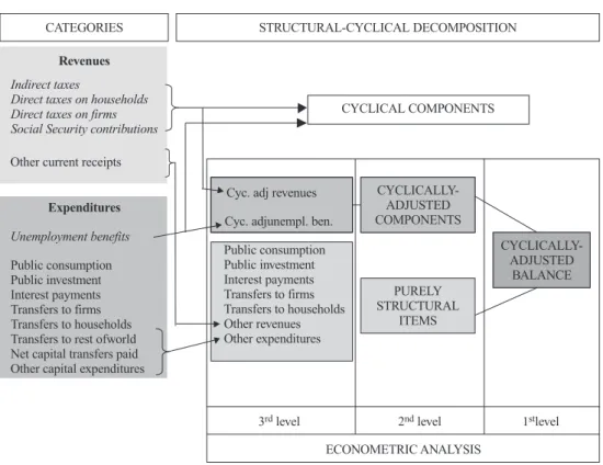
Obviously, should it hold thea prioribelief that observed budget balances depend on the output gap (GAP), this would show up in the correlation between both variables being signif-icantly different from zero. On the other hand, the very aim behind the calculations of CABs is to obtain a measure of the budgetary outcome that would be obtained when the public ac-counts are deprived of any cyclical influence (or, equivalently, when the output gap equals zero), so that statistically CAB and GAP should be uncorrelated. Then it follows that in case that some correlation would remain between the calculated CAB and the output gap, either the empirical method did wrongly remove the cyclical component from the observed balance or there exist some systematic discretionary policies that generate a cyclical behaviour. In figure 2 both the calculated CABs —obtained on the basis of the EC methodology— and GAPs are plotted for all EU countries but Luxembourg. Data has been taken from the AMECO database13. CABs are presented as a percentage of GDP, while the GAP is ex-pressed as a percentage of trend GDP. Although not conclusively, the graph allows to notice that, for several countries (notably, Germany or Greece) a negative correlation seems to exist between both variables, while seemingly the opposite would hold for Sweden. Besides, in the late 90's several countries could have converged towards a positive correlation.
The preliminary evidence just presented suggests that, for several countries, there is a re-markable correlation between the change in the structural or cyclically-adjusted balance and the cyclical position of the economy. Since the cyclical component of the balance is directly derived from the cyclical position, as it has been explained in section 3, this implies that, in many cases, the cyclical component of the deficit is not orthogonal to the structural compo-nent, signalling an anomaly in the computation of the former14. Such an anomaly may fun-damentally arise from two sources:
1) The first derives from the methodology used in the computation of the CAB, as per-formed by the EC (recall section 3) once the choice of the budgetary items that enter into the calculations has been made, but not from this choice itself. It may be possible that the estima-tion of the components of the budget balance which are assumed to display a cyclical pattern and to which we will refer asfiltered cyclical items,does not properly filter the cycle influ-ence out. For instance, it is quite possible that the actual behaviour of direct taxes is more (less) procyclical than actually estimated. This remaining cyclical component would be allo-cated to the CAB, inducing a positive (negative) correlation between the cycle and this struc-tural component of the budget balance. Therefore, the sign of the implied correlation be-tween the estimated cyclical components and the output gap isa prioriundetermined.
2) The second source regards the (assumed)purely structural items.Estimation of the cyclical components discards by assumption the possibility that some items of the budget, like public consumption and investment or transfers to firms, react to the position in the cy-cle. This is not necessarily true and their inadequate dismissal in the estimation may generate a significant correlation between the output gap and the structural components of the bal-ance, whose sign is also undetermined beforehand.
An additional source of correlation, which will be also addressed, arises from presenting the CAB relative to the actual GDP (Y), as it is done in many instances [see, for instance, European Commission (1995)], instead of relative to trend GDP (Y*), which is the right choice. To see why, assume that the economy is characterized by a zero trend real growth rate and zero inflation so that, in the absence of any discretionary measure, the nominal CAB would stay indefinitely at the same value. Assume besides that, in the initial period, the economy lies at its trend value. If, for instance, the economy moved above trend in the following period, measuring the CAB in terms of actual GDP would reflect a change in the structural balance (an improvement —worsen-ing— if the nominal CAB is negative —positive—), which is not correct; on the contrary, if the reference is done on the trend GDP the structural balance would remain constant.
5.
Metrics
The most direct way to explore these issues is to carry out a correlation analysis of the different components of the structural balance. However, it is quite straightforward and much more suitable to devise a simple methodology, based on regression analysis, to mea-sure quantitatively and systematically the effect of the cycle on each component. This allows us to consider all the countries in a panel and accounting for individual and heteroscedastic effects which renders the picture more precise. The analysis distinguishes three levels in the decomposition of the public balance, such as displayed at the bottom of the right-hand side in chart 1. The first level corresponds to the overall correlation between the CAB and the output gaps; the second level conveys the two sources of correlation identified in the previous sec-tion and the third level addresses the different components in the filtered cyclical and purely structural items, respectively. Finally, this methodology will also allow us to quantify the ef-fects of measuring the CAB related to actual instead of trend GDP. All the results will be
presented in differences, both to bypass potential problems of non-stationarity in the compo-nents and to allow for a more appealing interpretation of the parameters.
5.1.
Variance decomposition (first level)
Let us consider the following identity:DGAPº DGAP –DS +DS [7]
where, as explained in section III, is the difference between observed and trend output expressed in terms of the latter, and is the ratio of the cyclically-adjus-ted balance to trend GDP, orstructuralbalance ratio.
Multiplying both terms by the changes in the gap and applying the expectations operator we get:
E[DGAP2]ºE[DGAP(DGAP–DS)] +E[DGAP,DS] [8] which, taking into account thatE[DGAP] = 0, is equivalent to:
Var(DGAP)ºCov[DGAP, (DGAP–DS)] +Cov[DGAP,DS] [9] Finally, dividing the expression by the left-hand side term, we get:
1º bG+bS
where are the slope parameters of the following
regressions:
[10] If the computation of the cyclically-adjusted balance is properly done, it should be ex-pected thatDSis orthogonal to the changes in the output gap, so that the correlation coeffi-cient between both variables,r, is zero. SincebScan be written as a function of the
correla-tion coefficient, , a statistically null value forbSwill endorse the orthogonality
of the structural component and, hence, the adequacy of the decomposition. Equivalently, in this casebGwill equal one.
On the contrary, whenbSdiffers significantly from zero both components are found to
be correlated. The sign and significance of the parameter reveals the nature of the correla-tion: significant and positive values ofbSimply that the changes in the structural balance are
positively correlated with variations in the output gap, so that the structural balance is procyclical, while significant negative values imply a countercyclical behaviour of the struc-tural balance. * * Y Y Y GAP= -t t G G t Ct t S S t St GAP S GAP u S GAP u D - D = a + b D + D = a + b D + ( ) ( ) S Var S Var GAP D b = r D [ ,( )] [ , )] ( ) , ( )
Cov GAP GAP S Cov GAP S G Var GAP S Var GAP
D D -D D D D D b = b = * CAB Y S =
At first sight, this metric could be seen just as a more sophisticated way to compute the correlation between the variables. However, there are important advantages over a simple correlation analysis. The first apparent advantage is that using regression analysis allows to quantify how much does the structural balance respond to changes in the output gap:bScan
be interpreted as the percentage change (in terms of GDP) of the structural balance when the output gap increases by one percentage point of GDP. The second and more important ad-vantage is that, by decomposing the structural balance along the scheme of chart 1, it allows to identify and quantify the elements which determine the cyclical components in the struc-tural balance.
5.2.
Decomposition of the structural balance (second level)
Changes in the structural balance can be first decomposed into two components, as ex-plained in section 3:
SºSC+SX [11]
The first element,SC, contains the filtered cyclical elements andSXconveys the rest of
revenue and expenditure components which are not considered in the computation of the cy-clical balance, that is, the (assumed) purely structural components. Substituting the identity [11] into the final term in [7] and operating in an analogous way, the regression of the struc-tural balance on the output gap can be alternatively expressed by the following system of equations:
[12]
wherebSº bC+bX
Notably, this pair of identities reveal that the proposed metric permits to identify and quantify the factors which determine the correlation between the structural balance and the cycle. bX reflects how the purely structural components of the deficit are affected by the
changes in the output gap: ifbXturns out to be significantly different from zero, it means that
the components of the budget balance which have been considered purely structural do con-vey a cyclical content, opening the gate for their eventual consideration as cyclical compo-nents.bCreveals the sensitivity of the filtered cyclical items to the output gap variations:
val-ues forbCsignificantly different from zero would suggest that the cyclical filtering of the
public balance has been inadequate. The interpretation of the point estimates for theb's is the same as above.
5.3.
Further decomposition (third level)
Further insights can be attained by considering the different sub-entries ofScandSx. The
variableScincludes the five items whose behaviour is assumed to be cyclical (see section 2)
Ct C C t Ct Xt X X t Xt S GAP u S GAP u D = a + b D + D = a + b D +
after their estimated cyclical components have been filtered out. On the revenue side, this in-cludes the “structural” part of direct, indirect and corporate taxes, and social security contri-butions; on the expenditure side, it only includes the structural part of unemployment bene-fits. Our database does not include information on the cyclical component of each of the items, but only of the cyclically adjusted total revenues (denoted bySCR) and expenditure
(SCE). The purely structural balanceSxcontains the rest of items where the effect of the cycle
has not been filtered out. The database allows to distinguish among other current receipts (like special taxes, fees, etc. —SOR—), public consumption (SPC) and investment (SPK),
inter-est payments (SIP), transfers to firms (STF) and to households (STH) and other expenditures,
including net transfers to the rest of the world (SOE).
Hence, the parameter decomposition can proceed further within the two equations of the system [12], as follows:
[13]
for the first equation, withbCº bCR–bCE, and
[14]
for the second equation in [12], withbXº bOR–bPC–bPK–bIP–bTF–bTH–bOE. Signs have
been changed for expenditure items to allow for a more intuitive interpretation of the para-meters.
5.4.
Ratio bias
As noted above, the cyclically adjusted balance is sometimes inappropriately presented in terms of the actual GDP, instead of referencing it to the trend GDP. This introduces a wedge in the computation of the structural balance which is increasing with the size of the GDP gap and, therefore, it may affect the observed correlation between the cyclically ad-justed balance ratio and the output gap.
Quantifying the effect of using the inadequate ratio is quite straightforward within our methodology. Denoting the cyclically adjusted balance toactualGDP ratio bySY, to
distin-guish it fromS=CAB/Y*,we can write:
DSº DS–DSY+DSY CRt CR CR t CRt CEt CE CE t CEt S GAP u S GAP u D = a + b D + D = a + b D + ORt OR OR t ORt PCt PC PC t PCt PKt PK PK t PKt IPt IP IP t IPt TFt TF TF t TFt THt TH TH t THt OEt OE OE t OEt S GAP u S GAP u S GAP u S GAP u S GAP u S GAP u S GAP u D = a + b D + D = a + b D + D = a + b D + D = a + b D + D = a + b D + D = a + b D + D = a + b D +
and therefore, by operating as in the previous decompositions, bS º bY* + bY, where the
right-hand side parameters are estimated from the following system of equations:
[15] Thus,bYis the parameter which would be obtained if the CAB to actual GDP ratio is
used instead of the CAB to trend GDP ratio, andbY*does precisely pick up the distortionary
effect of using the inadequate ratio.
6.
Empirical results
After describing the estimation procedure, in this section we present the results of the analysis. Our main interest is to obtain an overall picture on the behaviour of the structural balance in the European Union countries for the available sample, obtained mostly from the AMECO database which covers from 1960 to 1998 (see footnote 13 and appendix A.2). The availability of a large number of countries with a relatively short sample leads us to analyse the evidence, in the first place, within a panel data framework. However, we will also con-sider two types of extensions: a moving average analysis, which sheds some light on the intertemporal changes in the behaviour of the structural components of the different budget entries, and an individual country analysis. Finally, we will address the effect of using the al-ternative ratios (nominal CAB to actual GDP v. nominal CAB to trend GDP).
6.1.
Panel results
The econometric specification is analogous to the previous systems of equations in a panel context, that is, introducing a cross-sectional dimension in the analysis. Note that it is impor-tant for the interpretability of the results to use parsimonious regressions, so that the parameter values (b) reflect precisely the impact of the cycle on the relevant fiscal item and, crucially, that they sum up to one. In any case, individual effects are considered in every equation; since the mean of the output gaps is zero, these individual effects capture the drift term in the struc-tural component considered for each country. A time dummy is also included, when signifi-cant, for the period 1994-98 due to the large and universal correction observed in EU deficits in their way to EMU. In contrast, autocorrelation of the series, which enter the regressions in dif-ferences, is low so we have not included lagged terms in the analysis.
The variance of the series considerably fluctuates among countries. Therefore, in a first step we estimated the equations by OLS —which is identical as using Seemingly Unrelated Regression Estimation [see, for instance, Greene (2000: 616)]—, and use the residuals to es-timate the variance for each country, which we use to correct for heteroskedasticity in the second step. Note that, in this second step, although the regressor (the output gap) is the same, it is not identical between equations because of the cross-sectional heteroskedasticity correction. Hence, estimating by SURE, which takes into account the cross-equation correla-tion matrix, results in a gain in efficiency.
* * *– – t Yt Y Y t Y Yt Yt Y Y t Yt S S GAP u S GAP u D D = a + b D + D = a + b D +
Panel results are shown in table 1 following the three-level scheme presented in the pre-vious section. Headings in the first three columns refer to each successive level, with entries under a given column showing parameter descriptions for that level. The presentation fol-lows a pattern in which scaled grey shaded areas are meant to help reading the results (with the darkest areas corresponding to first level entries).
Thefirst levelcorresponds to the estimation of system [10], that is the parametersbGand
bS. This allows us to check that their sum is one as theory suggests, although in table 1 we
only report the value ofbS. The significant estimate ofbSshows that European Commission
estimates of cyclically-adjusted balances are not orthogonal to the business cycle, which runs counter the conceptual underpinnings underlying their construction. More precisely, the CABs are found to be countercyclical and the parameter valuebS= –0.21 can be interpreted
as the percentage change in the structural balance-to-output ratio derived from a 1% change in the output gap. In particular, a 1% increase in the output gap worsens the assumed struc-tural balance by 0.21 percentage points of trend GDP15. Therefore the cyclically-adjusted balance is overstated in downturns and understated in expansions.
Thesecond levelis derived from the system [12], conveying the effect of changes in the output gap on the filtered cyclical items in the structural balance (bC), and on the purely
structural components of the balance (bX). The time dummy has only been included in the
former, since in the latter it is not significant. The results reveal that almost all the observed countercyclical behaviour of the structural balance is accounted for by the filtered cyclical
Table 1
LEVEL
PARAMETER
PANEL
First Second Third Parameter
value
t - ratio/ Dummie
Structural balance bs –0.209 –6.26 / *
Cyclically–filtered items bc –0.183 –6.91 / NO
Structural revenues from
cyclical items bcr –0.183
–7.16 / **
Structural expenditures
from cyclical items bce 0.019
1.49 / *
Assumed structural items bx 0.015 0.50 / *
Other revenues bor –0.007 –0.94 / * Public consumption bpc –0.017 –1.35 / * Public investment bpk 0.031 4.00 / NO Interest payments bip –0.017 –2.30 / * Transfers to firms btf –0.023 –2.76 / * Transfers to householdsa b th 0.007 1.14 / * Other expenditures boe –0.011 –1.08 / NO Ratio misspecification by* –0.025 –18.10
components. Indeed, the estimate forbC= –0.18 is negative and significant, and very close to
the previous estimate ofbS. On the contrary the estimation ofbX= 0.02 yields a positive but
insignificant value. Also note that the sum of both parameters is close tobS, as our
methodol-ogy suggests. These results are quite striking. On the one hand, they reject that the budgetary components which have been adjusted for cyclical influences are uncorrelated with the busi-ness cycle. Indeed, a 1% increase in the output gap results, for the whole panel, in a decrease of 0.18 percentage points in the ratio between these filtered items and trend GDP. Hence, since the adjusted cycle-sensitive items are countercyclical, it can be concluded that, over the cycle, the budget filteringoverstatesthe true size of its cyclical component (which is actually smaller). On the other hand, and contrary to our prior, the sum of the structural components is not in principle correlated with the output gap and overall, this would imply that it is ade-quate to keep these items away from filtering. A more in-depth analysis will allow us to qual-ify these conclusions, though.
Thethirdand finallevelof estimation jointly considers systems [13] and [14] to decom-pose the parametersbCandbXfurther, in order to discriminate among the different
sub-en-tries of the filtered cyclical and the purely structural items, respectively. In this last level, the two budgetary aggregates of cyclically adjusted items and assumed structural items are fur-ther decomposed into their respective individual items16.
As far as the filtered items aggregate is concerned, it is only possible to estimate the pa-rameters for total adjusted revenues (bCR) and total adjusted expenditures (bCE). The
insig-nificant value ofbCE= 0.02 indicates that the calculated structural part of expenditure in
un-employment benefits appears in fact to have been properly deprived of any cyclical influence17; on the other hand, and as a consequence, the estimate for total adjusted reve-nues (bCR= –0.18) accounts for the whole cyclical pattern observed in the filtered items of
the balance. We can then infer that the “excessive” filtering of the balance uncovered at the second level is fully explained by the elasticities used in the cyclical revenues items, which turn out to be too high. Unfortunately, the lack of disaggregated data on each item prevents us from individuating which element(s) are behind this result.
Regarding the purely structural items we could in principle figure out that, since their sum is insignificant, none of them will be significantly correlated to the gap. However, estimates for individual budgetary items which area prioriassumed to be unrelated to the cycle confirm that their aggregation conceals opposing effects stemming from the various items. In particular, public investment has been significantly procyclical (bPK= 0.03, implying that each
percent-age increase in the output gap is associated to an increase of 3 basis points in the public invest-ment to trend-GDP ratio); interest payinvest-ments and transfers to firms are slightly, but signifi-cantly, countercyclical, with parameter values around 0.02; on the contrary, other revenues, public consumption, transfers to households and other expenditures are insignificant.
6.2.
Moving average estimates
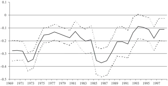
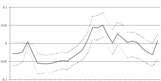
The sample spans for almost forty years, in which the fiscal behaviour of EU countries has been probably shifting through time. Thus, the convenience of implementing a more de-tailed time analysis. This is done by running rolling regressions in which extreme years change. We have chosen 10-year windows, so that the first regression covers 1960 to 1969, the second 1961-70, and so on. The estimation technique is the same as above, including the dummies after 1994. figures 3, 4 and 5 presents the results for the different estimates, refer-enced to the last included observation.
The point estimate for bS (figure 3) has been always significant but for the window 1985-94, ranging from around –0.35 (at the beginning of the sample and around the mid-eighties) to about –0.10 to –0.15 in the last decade. Before interpreting these results it is convenient to observe the estimates for higher levels of disaggregation.
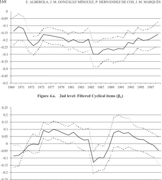
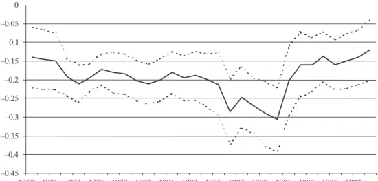
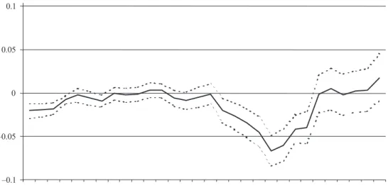
Filtered cyclical items estimates (bC) display a quite stable behaviour (figure 4.a), with a dip around 1985 (–0.3) and a slight upward trend thereafter, with a last estimate of –0.15. The estimates for cyclically-adjusted revenues (bCR), figure 4.b, basically mimic the pro-file ofbC, being always significant, whereas the profile of cyclically-adjusted expenditures (figure 5.a), v.g. unemployment benefits,bCE, is rather stable, being positive, although non significant, after 1975, and taking positive and significant values around 0.06 in the nineties.
On the contrary, the structural items estimates (bX) are quite volatile, taking negative and positive values which are non-significant in most cases (figure 4.b). However, as in the whole sample analysis, it is possible to distinguish among their components: public consumption shows a volatile behaviour (slightly negative and significant in the first half of the sample, positive but
Figure 3. 1st level: Cyclical Adjusted Balance (s)
–0.5 –0.4 –0.3 –0.2 –0.1 0 0.1 1969 1971 1973 1975 1977 1979 1981 1983 1985 1987 1989 1991 1993 1995 1997
insignificant in the final half —figure 5.c—); public investment started with insignificant values, but the parameter became positive (around 0.05) and significant after 1985 (figure 5.d); interest payments only showed a consistent negative and significant parameter between 1985 and 1992 (figure 5.e); finally, in a similar fashion to public investment, transfers to firms started being uncorrelated to the cycle, but after 1987 they have become significantly countercyclical taking the correspondingbTFparameter values around –0.04 (figure 5.f)18.
All in all then, the profile of thebSbasically mirrors the behaviour of the filtered cyclical
items, and in particular of the revenues. Notwithstanding this, other components of budget
Figure 4.a. 2nd level: Filtered Cyclical items (c)
Figure 4.b. 2nd level: Purely Structural items (x)
–0.5 –0.45 –0.4 –0.35 –0.3 –0.25 –0.2 –0.15 –0.1 –0.05 0 1969 1971 1973 1975 1977 1979 1981 1983 1985 1987 1989 1991 1993 1995 1997 1969 1971 1973 1975 1977 1979 1981 1983 1985 1987 1989 1991 1993 1995 1997 –0.25 –0.2 –0.15 –0.1 –0.05 0 0.05 0.1 0.15 0.2 0.25
balances have in certain periods influenced the behaviour of structural balances, like the countercyclicality of public consumption in the seventies, the procyclicality of investment from 1985 on, the shifting behaviour of transfer to firms (countercyclical since the late eight-ies) or the countercyclical behaviour of interest payments at the end of the eighties and the beginning of the following decade. Regarding the last periods, it is worth noting the declin-ing importance (in absolute value) of the cyclical revenues and the strong significance of un-employment benefits and public investment (both procyclical) which explains why the over-all value ofbShas been rather stable.
Figure 5.a. 3rd level: Cyclical Revenues (CR)
Figure 5.b. 3rd level: Cyclical Expenditures (CE)
1969 1971 1973 1975 1977 1979 1981 1983 1985 1987 1989 1991 1993 1995 1997 –0.45 –0.4 –0.35 –0.3 –0.25 –0.2 –0.15 –0.1 –0.05 0 1969 1971 1973 1975 1977 1979 1981 1983 1985 1987 1989 1991 1993 1995 1997 –0.5 –0.4 –0.3 –0.2 –0.1 0 0.1 0.2
Figure 5.c. 3rd level: Public Consumption (PC)
Figure 5.d. 3rd level: Public Investment (PK)
1969 1971 1973 1975 1977 1979 1981 1983 1985 1987 1989 1991 1993 1995 1997 –0.1 –0.05 0 0.05 0.1 1969 1971 1973 1975 1977 1979 1981 1983 1985 1987 1989 1991 1993 1995 1997 –0.1 –0.05 0 0.05 0.1
Figure 5.e. 3rd level: Interest Payments (IP)
Figure 5.f. 3rd level: Transfers to Firms (TF)
1969 1971 1973 1975 1977 1979 1981 1983 1985 1987 1989 1991 1993 1995 1997 –0.1 –0.05 0 0.05 0.1 1969 1971 1973 1975 1977 1979 1981 1983 1985 1987 1989 1991 1993 1995 1997 –0.1 –0.05 0 0.05 0.1
6.3.
Country analysis
The changing behaviour of fiscal policies and the emphasis on the global analysis led us to approaching the analysis from a panel perspective. However, in order to evaluate how general are these results, it is useful to contemplate, albeit briefly, how the parameters di-verge among countries. Table 2 displays the set of parameters for individual country equa-tions, which include a drift parameter and dummies after 199419. An additional column which states the number of countries for which each parameter is significant is also pre-sented.
The first thing to note is that, even when the panel results are very robust, the number of countries for which parameters are significant is low, as in the case ofbSorbC, with only
eight significant countries, or more clearly with public investmentbPKwith only three
coun-tries. Second, the range of the estimates is very wide and for certain parameters the sign even shifts. For instance, althoughbSis negative for all the countries in which the parameter is
sig-nificant, it ranges from –0.80 in Ireland to –0.17 in Finland;bXtakes a different sign in
Den-mark or Italy, and for higher levels of disaggregation the divergences increase, although the significant countries are less.
All in all, this variety of outcomes shows that comparing structural deficits among coun-tries should be taken with caution, since they are quite differently affected by the cycle and, also possibly, because of the small sample size.
We checked for the robustness of these results to changes in the methodology used to compute the CABs by applying this first level estimation to two alternative sets of CAB esti-mates. First, we did so for the Autumn 2002 AMECO database (even if the caveat from foot-note 13 applies). This database uses the OECD revised estimates of the CAB elasticities to the output gap (see footnote 10). Secondly, as it has been previously mentioned the European Commission has recently started to produce a different set of CAB estimates which are based on computing output gaps obtained under a production function methodology instead of trend-filtering the original series by making use of the Hodrick-Prescott filter. We have also replicated the estimation of thebsfor this second case.
The results of these two estimations are presented in the last two rows of table 3. In both cases, our previous results obtained when making use of the Autumn 2000 AMECO data broadly hold. This is specially time for the estimation results for CABs based on the Autumn 2002 AMECO database. As it can be seen in the second row in table 3, the same results in terms of statistical significance are obtained for all countries but Spain, for which the esti-mated parameter is now non significant20.
The last row of table 3 shows thebSestimates when making use of the CAB series
com-puted under the Commission's production function methodology. As it can be seen, for two more countries (Greece and Germany), the estimatedbsis now non-significant. The previ-ous results hold for the other countries in the table in terms of statistical significance (albeit sometimes with non-negligible differences in the point estimates).
Table 2 Country regressions: parameter value Paramete r No. o f significant Bel D en Fin Ita Irl Swe Aus U.K. Por N et Fra Spa Gre Ger bS 8 –0.30* 0.08 –0.17* 0 .02 – 0.80* 0.03 –0.07 –0.42* –0.04 –0.46* –0.03 –0.21* –0.25* –0.35* bC 8 –0.27* –0.09 –0.22* –0.11 –0.78* 0.27 –0.14* –0.50* –0.10 –0.50* –0.12 –0.14 –0.19* –0.14* bCR 7 –0.35* 0.13 –0.20 –0.09 –0.65* –0.13 –0.15* –0.38* –0.06 –0.35* –0.16 –0.06 –0.11* –0.31* bCE 4 –0.08 0.21* 0 .00 0 .01 0 .11 –0.38 –0.00 0.12 0.03 0.14* –0.04 0 .06 0 .07* –0.17* bX 4 0 .06 –0.30* 0 .13 0 .18* –0.15 0 .24 0 .13 –0.05 0.03 –0.16 0 .19* –0.13 –0.11 –0.03* bOR 2 –0.00 0.01 –0.03 0.01 0.03 –0.04 0.02 0.00 0.04* 0.02 –0.01 –0.04 –0.03* 0 .01 bPC 2 –0.03 –0.10 –0.03 –0.00 0.09 –0.01 –0.01 –0.08* 0.04 0.01 –0.06* 0.03 –0.03 0.03 bPK 3 –0.00 0.00 0.01 –0.01 0.07 0.08 0.03 0.06* 0.02 0.02 0.03 0.05 0.06* 0 .07* bIP 2 –0.00 0.08 –0.05* –0.02 0.08 –0.08 –0.01 0.02 –0.01 –0.03 – 0.05* –0.03 –0.04 –0.02 bTF 4 0 .00 0 .04* –0.01 –0.12* 0.17* –0.02 –0.05* –0.05 –0.06 0.03 –0.08 –0.02* –0.03 0.03 bTH a 3 0 .07 0 .23 –0.18* 0 .10 – 0.04 0.52 –0.13 –0.20* –0.01 0.19 –0.04 0 .05 0 .10* 0.06 bOE 5 –0.02 –0.05 0.00 –0.04 –0.25* –0.32* –0.01 0.05 –0.03 –0.13* 0.07* –0.03 0.01 0.08* bY * 1 3 –0.06* –0.00 –0.02 –0.09* –0.07* –0.01* –0.01* –0.03* –0.02* –0.04* –0.02* –0.04* –0.02* –0.02* a Data obtained for 1985-1998 * S ignificant at 9 5 % and * * at 9 0%
Table 3 Country regressions: robustness checks Parameter No. o f significant Bel D en Fin Ita Irl Swe Aus U.K. Por N et Fra Spa Gre Ger bS (baseline: OGs and C ABs obtained from the Spring 2000 AMECO d ata-base) 8 –0.30* 0.08 –0.17* 0.02 –0.80* 0 .03 – 0.07 –0.42* –0.04 – 0.46* –0.03 –0.21* –0.25* –0.35* bS (OGs and C ABs obtained from the Autumn 2002 AMECO d atabase, H-P filter b ased) 7 –0.32* –0.06 – 0.17* 0.08 –0.52* 0 .15 0 .1 –0.32* 0.01 –0.39* 0.05 –0.01 –0.19* –0.22* bS (OGs and C ABs obtained from the Autumn 2002 AMECO d atabase, production function b ased) 5 –0.32* –0.08 – 0.2* 0.08 –0.46* 0 .18 0 .01 –0.33* 0.01 –0.37* 0.1 – 0.01 –0.2 –0.16 a *S ig n if ic an ta t9 5% .
Thus, we can safely conclude that the basic message of this paper (namely, that CABs show a cyclical behaviour) is robust enough to changes in the methodology used to calculate the CABs.
6.4.
Ratio choice
The choice of presentation of the ratio also introduces a cyclical bias in the estimation of the CAB balance, as explained in section 5.4. At the bottom of table 1 we observe that
bY*= –0.025 and that it is highly significant, that is, if the ratioCAB/Yis used instead of the
CAB/Y*ratio, the correlation between the output gap and the structural balance would de-crease: since the structural balance is countercyclical (bS = –0.21) this implies that bY
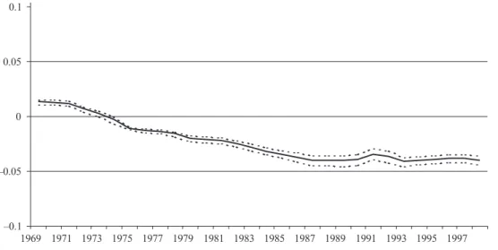
—the resulting parameter of regressing the changes in the CAB/Y ratio with respect to the changes in the output gap (see [15])— would be around –0.185. A look at the moving aver-age estimates ofbY*(figure 6) shows that they change from positive to negative after 1975,
stabilising by the end of the sample at around –0.04. Finally, when the exercise is done country-by-country, the parameters are also negative for all the countries but Finland, which is the only country which has run, on average, structural superavits for the whole pe-riod (see figure 2); the highest values (in absolute value) correspond to Italy and Belgium, which are the countries with highest average structural deficit in the sample.
All these results indicate that the sign of the parameters is associated with the sign of the cyclically-adjusted balance, whose negative behaviour in most of cases determines the nega-tive signs obtained in the analysis21.
Figure 6. Mismeasurement Ratio (bY*)
1969 1971 1973 1975 1977 1979 1981 1983 1985 1987 1989 1991 1993 1995 1997 –0.1 –0.05 0 0.05 0.1
All in all, the estimation of the parameter related to using the CAB/Y ratio suggests a quite paradoxical inference: although in principle it is more adequate to use the CAB/Y* in order to assess more precisely structural balances, the fact is that using the inappropriate CAB/Y reduces the countercyclicality of the CABs, implying that it corrects to some extent the misadjustement of the structural balance.
7.
Conclusions
The aim of this paper goes beyond checking whether the cyclically adjusted balances (CABs) —as calculated by the European Commission through its Hodrick-Prescott method— retain some cyclical behaviour. It is a formal attempt to assess through which bud-getary items the cycle impinges on the CAB and to provide a quantitative and intuitive mea-sure of such impact.
In the panel framework including EU countries, our results indeed show that there is a negative and significant correlation between the output gap and the structural balance: an in-crease in the output gap equal to 1% of GDP reduces the computed structural balance by 0.21% points of GDP. This implies that the cyclical component is overestimated and, as a re-sult, in downturns structural balances tend to be overestimated and, conversely, in expan-sions they are underestimated. The dominant source of this distortion arises from the filtering of revenues deemed to be cyclical, possibly signalling a problem with the computation of elasticities which turn out to be too high. An alternative possibility is for our estimates to be capturing a systematic discretionary reaction on the side of the authorities to developments in economic activity. However, it does not appear easy to disentangle between both possibil-ities. To do so, one would need to check exhaustively for changes in the legal provisions be-hind these cyclically-filtered items. Further, this paper does not put into question the way in which the European Commission computes the output gap. However, one possible reason for the overstatement of the cyclical component of budget balances might lie with the choice of the value for the parameter l when observed output is decomposed through the Hodrick-Prescott filtering technique into its trend and cyclical components. Bearing in mind that the larger the value ofl is, the larger are the deviations of observed output from its trend, our results might be suggesting that the value ofl = 100 adopted by the European Commission would be too large.
As far as the items which are assumed to contain no cyclical components are concerned, their joint effect is non significant, but this overall result conceals offsetting effects in some items; more precisely, public investment turns to be significantly procyclical and interest payments and transfer to firms are countercyclical. These latter results do not necessarily mean that cyclical comovements in assumed structural items are the result of the presence of built-in automatic stabilizers in the corresponding budgetary entries. On the contrary, they could be explained, as in the case of cyclically-filtered items by the implementation of sys-tematic discretionary policies.
The extensions of the empirical analysis provide interesting hindsights, too. First, the variability of the parameter estimates using a rolling regression procedure suggests that the relationships are not stable. Furthermore, while the usual practice of estimating the elastici-ties for a given recent period and then applying them backwards may be suitable in common uses of CABs (since most often the interest lies in the analysis of the most recent periods), it may indeed be important in order to explain the non-stability of our estimated relationships. Second, the large differences in results among countries provides a note of caution regarding the comparison of structural balances among countries. Last but not least, quite paradoxi-cally, it may be convenient to use the ratio of cyclically-adjusted balances to nominal GDP, instead of to trend GDP which is more correct, because otherwise the distortion due to the cycle would be even higher in absolute terms (b= –0.21% instead ofbY= –0.18%).
To summarize, the results presented in this paper show that estimates of the cyclically adjusted budget balances may be subject to considerable uncertainty, given the theoretical and empirical limitations associated with their definition and calculation. Thus although these indicators can play a useful role in assessing and formulating fiscal policy they should be interpreted with caution. This is especially important in the current EMU framework, where CABs have become an important tool in determining the compliance of countries with the Stability and Growth Pact.
Appendix A.
The different items in the general government accounts
Indirect taxesare payments made to the general government in connection mainly with the production and importation of goods and services. Since they are proportional to the size of production, indirect tax revenue in nominal terms fluctuates with the business cycle around some trend provided that there are no normative changes (i.e. modifications of tax bases or rates).
Direct taxesare payments made to the general government which are assessed upon the income and wealth of economic agents. They may include as well some periodic taxes not raised from income and wealth. Apart from the last component, direct tax revenues fluctuate as well with the economic cycle. Direct taxes are paideither by households or by firms.
Social security contributionsare composed of the (actual) social contributions paid by employers, employees, self-employed and, possibly, non-employed people to social security funds plus the so-called imputed social contributions. The latter are the counterpart of social benefits paid by general government units to their employees or other eligible people. Since employment is positively correlated with the cycle, total social security contributions are as well an obvious candidate for cyclical adjustment.
Other current receiptsis an heterogeneous grouping of entries covering property income (such as interest received, rents and dividends paid by public enterprises to government units), various current transfers received (including those arising, for instance, from fines and penalties or from current international cooperation) and, finally, the gross operating sur-plus obtained by government units from their market production activities.
Government consumptionis, in turn, composed of the compensation of public employ-ees and current purchases of goods and services. The compensation of public employemploy-ees ac-counts for the total remuneration payed by government units to their employees, which in-cludes gross wages and salaries plus employers' actual social contributions and imputed social contributions. Current purchases of goods and services are computed net of sales of goods and services and excluding the consumption of fixed capital.
Current transfers to householdsembraces social benefits made available by government units with the aim to cover, as a general rule, the appearance of certain risks or needs which would otherwise impose a financial burden on families.Unemployment benefit paymentsare one of the elements included within this category.Current transfers to firmsare production and import subsidies made by the general government to economic agents producing or im-porting goods and services.Current transfers to the rest of the worldare computed in net terms (that is, as the difference between those paid by the government to the rest of the world and those received from it).
Actual interest payments comprise the remuneration of financial assets issued by the general government and held by other sectors.
Final capital expenditureis composed of three items: gross fixed capital formation (the value of durable goods which are acquired to be used for a period longer than one year), net purchases of land and intangible assets, and changes in strategic or emergency stocks or held by market regulatory agencies.
Finally,net capital transfers paidare the net result of those paid (investment grants, un-requited transfers by general government or by the rest of the world to finance gross fixed capital formation) and those received (investment grants received, taxes on inheritances, on gifts and, only if levied occasionally, on assets and net worth).
Appendix B.
Data
The data used in this paper has been taken from the AMECO database and covers the pe-riod 1960-2000. It should be noted, however, that figures for the last two years correspond to estimations or forecasts provided by AMECO. For this reason, the sample in some regres-sions does not go beyond 1998. The dissagregation of the general government accounts pro-vided in AMECO nearly suffices for the purpose of this work. However, for some items, it has been necessary to resort to a different database, which requires to deal with a problem of compatibility among different sources. In particular these problems arise for the following items:
— The AMECO database only contains information about aggregated direct tax revenue collected by the general government. However, the disaggregation between revenue accruing from taxes paid respectively by households and firms is deemed relevant since, as it was pointed out in section 3, the two categories enter separately into the calculations of the CAB performed by the EC. On these grounds we obtained this
in-formation from the «Revenue Statistics» published by the OECD. Nevertheless, total direct tax revenue in this publication and in AMECO do not match each other. To deal with this problem, the respective shares of direct taxes falling upon firms and households from the OECD source are extrapolated to the AMECO totals.
— The AMECO database does not present separate data on unemployment benefit pay-ments. The concept closest to the unemployment compensation in AMECO corres-ponds to «Transfers to households», but this is a wide category that includes, among other subentries, the pension payments. Again, we obtained some information in OECD publications about the unemployment-related payments, whose use poses a problem which is similar in nature to the one just described. The same modification as before is implemented. However, since the information from the OECD begins in 1985, the analysis involving unemployment compensation only covers a subsample starting that year.
— The data for Germany contained a specific problem related to the discontinuity of the series brought about by the reunification. Prior to 1991 just information for West Germany can be collected, while for 1991 series both for West Germany and for the Unified Germany are available and, from 1991 on, only information about the last one can be obtained. In addi-tion, the rest of the information (for example, that on elasticities) corresponds to Germany as a whole. Then the choice has to be made either to consider Germany and West Germany as different countries and make the analysis separately, or to extend the series for West Ger-many beyond 1991 with the growth rates recorded for GerGer-many. The second alternative has been selected, which implies that the unification process for Germany only gives rise to a change in the level but not in the evolution of GDP and the fiscal variables.
Notes
1. More precisely, it has often been proposed to assess the fiscal stance on the basis of the changes in the cycli-cally-adjustedprimarybalance rather than the changes in thetotalcyclically-adjusted balance.
2. Throughout the paper, the behavior of a given budgetary component is said to be countercyclical (procy-clical) if its changes show a negative (positive) correlation with the changes in the output gap. Thus, countercyclical and procyclical patterns are not defined here with regard to the impact of fiscal policy on the economy.
3. The new AMECO database provides long series that unfortunately are not always fully compatible. In particu-lar for those periods previous to 1995, the GDP series has been transformed by using the growth rate observed for the variable in ESA 79 but making the level compatible with the ESA 95. The public finance variables re-ported in new AMECO do not have this transformation, therefore all the ratios between fiscal public finance variables and GDP reported in this database should be conducted carefully.
4. Appendix A.1 contains precise definitions for each revenue or expenditure category.
5. In principle,capital transfers receivedshould be considered as a further (capital) revenue item. Nevertheless, these are presented in our database as a negative expenditure within the wider category of expenditure labeled
net capital transfers paid.
6. In recent years, the European Commission has been using in its publications and in the yearly assessment of the Stability and Convergence programmes a method based on a smoothing technique. This is the method
un-derlying the empirical analysis in this paper. As recently as this year, the Commission has devised a new met-hod based on the calculation of a production function. It is likely that this new metmet-hod will tend to become gra-dually the single one used by the Commission in their analyses. However, for the time being, both methods are set to coexist. Interestingly, both EC methods tend to provide very similar results in terms of calculated output gaps, the reason being that most of the variables entering the calculation of the production function are H-P fil-tered so that, in practice, the production function method developed by the EC is not very different from its H-P method.
7. Calculated as in equation 3, that is as the quotient of the difference between actual GDP and trend output, and this latter variable.
8. Indeed, the fact that the four adjusted revenue categories are scaled by total revenue (instead of being scaled by the sum of these four revenue groups) is equivalent to assuming that the elasticity of the two remaining re-venue categories is zero.
9. The weights are calculated as an average of the period 1980-1992. Note that the cyclical component of public revenue does not only depend on the elasticity of revenue but also on their share in GDP since the output gap is multiplied by the actual yearly revenue share of GDP. However, given that the revenue elasticity is calculated as a weighted average of the respective elasticities of each of the revenue groups considered and the weight of each revenue component is calculated as an average of a certain period, the method does not take into account the effects of shifts in the composition of public revenues.
10. Note that elasticities are assumed to remain constant over time, since the same elasticities are applied to the whole period of available data. Elasticity estimates are occasionally revised, but this does not imply applying different elasticities to different periods of time since the new elasticities are applied to all periods of time in order to calculate cyclical components. The OECD has recently revised the method of calculating the elastici-ties (Van den Noord, 2000). However, the series used in this paper were published by the European Commis-sion before the new OECD elasticities were available. For this reason, we refer above to the previous OECD method for estimating elasticities.
11. The OECD adjusts this elasticity for the collection lags in corporate taxes identified in some countries. 12. Note that, in the case of expenditure and in contrast with revenue, the cyclical component does not depend on
the share in GDP of actual yearly unemployment outlays. Thehandmparameters are estimated over a long period and assumed constant.
13. See Appendix A.2 for more details. One important issue to be stressed is that we have used the AMECO data-base data-based on ESA-79 instead of the more recent one built under ESA-95 accounting standards, given the fact that long time series do not exist in this case. To be more precise, the ESA-95 version of the AMECO database contains only data for the most recent periods (from 1995 onwards). Although these series have been extended backwards, the extension methodology presents serious problems, so that data before and after 1995 are not fully compatible. In particular, for periods before 1995, the GDP series have been obtained by applying to the level of the series in that year the growth rates observed for this variable under ESA-79. An analogous trans-formation has not been undertaken for public finance variables. Thus there is a break in the level of these se-ries in 1995. As a consequence, for the ESA-95 AMECO database, the ratios between public finance variables and GDP prior to 1995 are not very meaningful.
14. Again, there may be nothing wrong in the computation if, for instance, governments tend to engage in fiscal consolidation processes in the upper part of the cycle. In this case, a positive correlation between the OG and the CAB would still be consistent with having removed the impact of the cycle from the observed balance 15. The (unreported) estimate of thebGis 1.20, which implies thatbs+bG»1.
16. Only forpublic investmentand for the categoryother expenditures,dummies have not been included. 17. Note, however, that data on this item have to be taken with caution. See appendix A.2.
18. The behavior of the rest of components is not remarkable, so we do not present them in the graphs. 19. Obviously, country level heteroskedasticity correction does not apply in this case.