Direct Numerical Simulation of Acoustic Disturbances in the
Rectangular Test Section of a Hypersonic Wind Tunnel
Cole P. Deegan∗, Junji Huang†and Lian Duan‡
Missouri University of Science and Technology, Rolla, MO 65409 Meelan M. Choudhari§
NASA Langley Research Center, Hampton, VA 23681
Direct numerical simulations (DNS) of the full-scale rectangular nozzle of a hypersonic wind tunnel are conducted to study the acoustic freestream fluctuations radiating from turbulent boundary layers (TBLs) along the nozzle walls. The nozzle geometry and the flow conditions of the DNS match those of the NASA 20-Inch Mach 6 Tunnel, and the DNS has been completed for a domain without spanwise sidewall boundary conditions. The turbulent boundary layer parameters based on the DNS compare well with those derived from Reynolds Averaged Navier-Stokes (RANS) calculations as well as with the predictions based on Pate’s correlation. A similarly good comparison is observed for both the Mach number distribution and the Reynold’s stresses obtained from the DNS and RANS calculations, respectively. Various characteristics of the acoustic pressure fluctuations within the inviscid core of the nozzle flow are compared with those associated with a single flat plate at a similar freestream Mach number. The frequency spectrum and bulk propagation speeds match well between the nozzle and the flat plate, but the rms pressure fluctuation is higher for the nozzle configuration, likely due to the combined effect of acoustic radiation from the top and bottom walls. Spatial contours of the two-point correlation coefficient display elliptical tails with approximately equal but opposite angles corresponding to the preferred directionality of acoustic structures radiated from both walls. Future work will focus on DNS of the full nozzle configuration, including the effects of the nozzle side walls.
Nomenclature
Cp = heat capacity at constant pressure, J/(K·kg)
Cv = heat capacity at constant volume, J/(K·kg)
H = shape factor,H=δ∗/θ, dimensionless
M = Mach number, dimensionless
Mr = relative Mach number,Mr =(U∞−Ub)/a∞, dimensionless
Pr = Prandtl number,Pr =0.71, dimensionless
R = ideal gas constant,R=287, J/(K·kg), or radius of the axisymmetric nozzle, m
Reunit = unit Reynolds number,Reunit ≡ρ∞U∞/µ∞, 1/m
Reθ = Reynolds number based on momentum thickness and freestream viscosity,Reθ ≡ρ∞U∞θ/µ∞, = dimensionless
Reδ2 = Reynolds number based on momentum thickness and wall viscosity,Reδ2≡ρ∞U∞θ/µw, dimensionless Reτ = Reynolds number based on shear velocity and wall viscosity,Reτ≡ρwuτδ/µw, dimensionless
rms = root mean square
T = temperature, K
Tr = recovery temperature,Tr=T∞(1+0.9∗γ−12 M∞2), K
U∞ = freestream velocity, m/s
Ub = bulk propagation speed of freestream acoustic disturbances, m/s ∗Graduate Student, Student Member, AIAA
†Graduate Student, Student Member, AIAA ‡Assistant Professor, Senior Member, AIAA
§Aerospace Technologist, Computational AeroSciences Branch, M.S. 128. Associate Fellow, AIAA
a = speed of sound, m/s p = pressure, Pa q = dynamic pressure, Pa r = radial coordinate u = streamwise velocity, m/s uτ = friction velocity, m/s v = spanwise velocity, m/s w = wall-normal velocity, m/s
x = streamwise direction of the right hand Cartesian coordinate
y = spanwise direction of the right hand Cartesian coordinate
z = wall-normal direction of the right hand Cartesian coordinate
zn = wall-normal distance, m
zτ = viscous length,zτ =νw/uτ, m
γ = specific heat ratio,γ=Cp/Cv, dimensionless
δ = boundary layer thickness, m
δ∗ = displacement thickness, m κ = thermal conductivity,κ=µCp/Pr, W/(m·K) θ = momentum thickness, m µ = dynamic viscosity,µ=1.458×10⁻⁶T+T1103/2.4, kg/(m·s) ν = kinematic viscosity,ν=µ/ρ, m2·s ρ = density, kg/m3 = Subscripts =
i = inflow station for the domain of direct numerical simulations
rms = root mean square
w = wall variables
∞ = freestream variables
t = stagnation quantities
= Superscripts =
+ = inner wall units
(·) = averaged variables
(·)0
= perturbation from averaged variable
I. Introduction
The elevated freestream disturbance levels in conventional (i.e., noisy) high-speed wind tunnels usually result in an earlier onset of transition relative to that in a flight environment or in a quiet tunnel. Yet, the conventional facilities continue to be used for transition sensitive measurements because of the size and Reynolds number limitations of existing quiet facilities and the prohibitive cost of flight tests. To enable a better use of transition data from the conventional facilities, it is important to understand the acoustic fluctuation field that dominates the freestream disturbance environment in those facilities. With increased knowledge of the receptivity mechanisms of high-speed boundary layers [1, 2], it becomes particularly important to characterize the details of the tunnel acoustics originating from the tunnel-wall turbulent boundary layers.
Direct numerical simulations (DNS) of the acoustic fluctuation field radiated from tunnel-wall turbulent boundary layers can overcome a number of difficulties encountered during experimental measurements of tunnel freestream disturbances and also provide access to quantities that cannot be measured easily [3–5]. Successful application of DNS for capturing the freestream acoustic pressure fluctuations has been demonstrated for spatially-developing turbulent boundary layers over a flat plate at Mach 2.5–14 [6–9] and on the inner wall of axisymmetric nozzles [10, 11]. These flat-plate simulations have the benefit of isolating more easily the acoustic radiation from a single surface, thus facilitating a comprehensive understanding of the genesis of freestream disturbance field and its dependence on boundary-layer parameters (e.g., freestream Mach number, wall temperature, Reynolds number), while the simulations within an axisymmetric nozzle allow for combined characterization of noise generation and reverberation within axisymmetric tunnel-nozzle flows.
Many operating hypersonic wind tunnels including the NASA 20-Inch Mach 6 Tunnel are, however, nonaxisymmetric with a rectangular nozzle. As a result, the freestream disturbances in such tunnels reflect the combined outcome of acoustic radiation from the four nozzle walls and the corners between them. The process of acoustic reverberation within such nozzle configurations controls the spatio-temporal characteristics of freestream disturbances. It is likely to be different from that in axisymmetric wind tunnels and remains largely unknown as yet. To understand the wind tunnel acoustic environment in rectangular nozzles and to provide insights into the similarities and differences in freestream noise properties between hypersonic wind tunnels with rectangular and axisymmetric nozzles, the present research effort seeks to simulate the acoustic radiation within a rectangular nozzle. As an initial step toward that goal, this paper outlines the results of a preliminary DNS with the same convergent-divergent nozzle contour as that of the NASA 20-Inch Mach 6 Tunnel but without the two spanwise side walls. This simpler configuration provides a useful reference for characterizing the dependence of acoustic noise generation and reverberation on the multiple walls comprising the tunnel surface and helps isolate the effects of spanwise side-walls and corners on acoustic noise generation and reverberation.
The paper is structured as follows. The flow conditions and numerical methods are outlined in Section II. Section III presents the comparison of DNS results against the full-tunnel Reynolds-Averaged Navier-Stokes (RANS) solution obtained by the VULCAN [12] code as well as preliminary DNS predictions of freestream acoustic noise characteristics. A summary of the overall findings is given in Section IV.
II. Flow Conditions and Numerical Methodology
Targeted flow conditions within the test section are summarized in Table 1, which fall within the range of nozzle conditions of the NASA 20-Inch Mach 6 Tunnel. The wall temperature is 300 K, corresponding to a wall-to-recovery temperature ratio ofTw/Tr ≈0.64.
Table 1 Nominal freestream conditions for the NASA 20-Inch Mach 6 Tunnel. M∞ U∞(m/s) ρ∞(kg/m3) T∞(K) Tw(K) Pt(KPa) Tt(K) Reunit(1/m)
5.9 948.1 0.033 64.3 300 873.3 511.6 2.0×10⁶
A. Governing Equations and Numerical Methods
The full three-dimensional compressible Navier-Stokes equations in conservation form are solved numerically in generalized curvilinear coordinates, describing the evolution of the density, momentum, and total energy of the flow. The working fluid is assumed to be a perfect gas and the usual constitutive relations for a Newtonian fluid are used: the viscous stress tensor is linearly related to the rate-of-strain tensor, and the heat flux vector is linearly related to the temperature gradient through Fourier’s law. The coefficient of viscosityµis computed from Sutherlands’s law, and the coefficient of thermal conductivityκis computed fromκ=µCp/Pr, with the molecular Prandtl numberPr =0.71. A detailed description of the governing equations can be found in Wu et al. [13].
The inviscid fluxes of the governing equations are computed using a seventh-order weighted essentially non-oscillatory (WENO) scheme. Compared with the original finite-difference WENO introduced by Jiang and Shu [14], the present scheme is optimized by means of limiters [13, 15] to reduce the numerical dissipation; WENO adaptation is limited to the boundary-layer region for maintaining numerical stability while the optimal stencil of WENO is used outside the boundary layer for optimal resolution of the radiated acoustic field. The viscous fluxes are discretized using a fourth-order central difference scheme and time integration is performed using a third-order low-storage Runge-Kutta scheme [16].
For the inlet boundary condition, a digital-filter based method [17, 18] is applied. The mean profiles, Reynolds stress tensor, and integral lengths required by the digital-filter method are obtained from a precursor RANS calculation that simulates the full-domain tunnel geometry. The details of the RANS will be discussed in Section II.B. No-slip conditions are applied for the three velocity components on the wall and an isothermal condition is used for the temperature. At the outlet boundary, unsteady nonreflecting boundary conditions based on Thompson [19], together with a fringe zone with streamwise stretched meshes, are used to avoid acoustic reflections at the boundary. Periodic boundary conditions are used in the spanwise direction, given the absence of spanwise side-walls. The DNS will be referred to as Case “DNS-No Sidewalls” in the remainder of the paper.
The details of the DNS methodology have been documented in our previous simulations of acoustic radiation from turbulent boundary layers [6, 7, 9–11]. The DNS solver has been previously shown to be suitable for computing transitional and fully turbulent flows, including hypersonic turbulent boundary layers [20, 21], the propagation of linear instability waves in 2D high-speed boundary layers, and secondary instability and laminar breakdown of swept-wing boundary layers [22, 23].
B. Simulation Setup
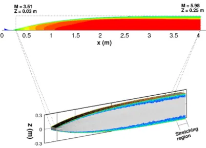
RANS computations of the tunnel flow-field were performed using the VULCAN code to characterize the turbulent boundary layer flow regime. The RANS calculations simulate the full tunnel geometry, including the converging and diverging nozzle sections that lead up to the test section. The flow is assumed to be fully turbulent throughout the nozzle; and the Reynolds stresses and turbulent heat flux are modeled via Menter’s two-equation, shear-stress-transport (SST) turbulence model. As seen in the top of Figure 1, the tunnel configuration starts with the converging section in advance of the nozzle throat, which is located atx≈0.18 m. The diverging section spans from x≈0.18 m tox≈3.67 m, followed by the test section region. The RANS simulation with and without tunnel side walls will be referred to as Case “RANS-With Sidewalls” and “RANS-No Sidewalls”, respectively, in the remainder of the paper.
The diverging section of the tunnel nozzle was then simulated using DNS. As seen in the bottom of Figure 1 the DNS domain in thex−zplane corresponds to a subset of the RANS domain and starts slightly downstream of the nozzle throat atx=0.265 m, where the local freestream Mach number isM∞=3.00, and ends at the nozzle exit at
x=3.67 m, where the freestream Mach number isM∞=5.93. Given the streamwise extent of the DNS domain and the known, rapid increase in acoustic radiation with increasing Mach number at the boundary-layer edge, we believe that the selected DNS domain encompasses the origin of most of the acoustic sources responsible for generating the freestream noise inside the test section. The streamwise length of the DNS domain is 47.8δr, whereδr is the boundary layer thickness at the nozzle exit from the results of RANS-No Sidewalls, and is equal to 0.0684 m. To prevent the reflection of any acoustic disturbances produced by the outflow boundary condition back into the flow regime of interest, an extra region was appended to the DNS domain.
Table 2 Domain and mesh parameters for Case DNS-No Sidewalls
Case xi(m) xe(m) Lx(m) Nx Ny Nz Lx/δr Rexit/δr ∆xmax+ ∆y+max ∆z+wall ∆z+in f DNS-No Sidewalls 0.3 3.58 3.27 4000 400 1199 47.8 3.7 11.61 5.39 1.07 7.44
This appended region consists of an additional 30 streamwise grid points and the streamwise grid spacing is progressively stretched across the length of this region by using a stretching ratio of 1.1. Table 2 lays out the grid size and grid resolutions of the DNS mesh.
III. Results
In this section, the RANS and DNS results for the nozzle-wall turbulent boundary layer as well as the DNS predictions of freestream acoustic field are presented. First, the mean turbulent statistics within the boundary layer are compared among all the DNS and RANS cases along with the results derived from empirical relations such as the Pate correlation [24]. Next, preliminary results of boundary-layer-induced pressure statistics are analyzed for the DNS.
Table 3 lists the properties of nozzle-wall turbulent boundary layer at the nozzle exit (x=3.67 m). Four sets of results are included in the table: two based on the RANS calculations (Case RANS-No Sidewalls and Case RANS-With Sidewalls), one based on the DNS (Case DNS-No Sidewalls), and one based on empirical estimates derived from Pate’s correlation [24]. The latter correlation allows one to deduce the boundary layer displacement thickness,δ∗, and the nozzle wall friction coefficient,Cf. The shape factorH, boundary-layer thickness, and the momentum thickness of the tunnel-wall boundary layer, as well as the Reynolds numbers based on these parameters, are then estimated using an empirical relation by Wood [25] and a power law profile with an exponent of 1/9 [26]. Overall, favorable comparisons in boundary-layer parameters are found among the DNS, the RANS, and the empirical relations, especially among the DNS and RANS results. In particular, the noticeably larger boundary-layer thickness for Case RANS-With Sidewalls is likely due to spanwise confinement effects in the presence of the nozzle’s corners and side-walls.
Fig. 1 Computational domain set up for (top) RANS, contours colored by Mach number, and (bottom) Case DNS-No Sidewalls, shown as numerical schlieren image with contours colored by the magnitude of vorticity to emphasize the large-scale motions within the boundary layer. The nozzle shape shown in the figure has been nonuniformly distorted from the actual contour, while preserving the qualitative shape of the wind tunnel configuration.
Table 3 Boundary layer properties at nozzle exitx=3.67m. Boundary-layer parameters for Case RANS-With Sidewalls are based on the wall-normal profile within the plane of spanwise symmetry of the tunnel cross section.
Case M∞ Reunit(1/m) Tw(K) TTwr Reθ Reτ Reδ2 δ(mm) δ ∗ (mm) H zτ(µm) cf(10−3) Pate 6.0 2.0×10⁶ 300 0.64 18762 1159 4552 68.1 35.94 12.3 58.8 1.15×10⁻³ RANS-No Sidewalls 5.98 2.0×10⁶ 300 0.64 29341 995.4 6682 68.4 32.09 7.7 68.8 7.91×10⁻⁴ RANS-With Sidewalls 5.87 2.0×10⁶ 300 0.64 30725 1220 7219 78.2 29.34 7.0 64.0 7.42×10⁻⁴ DNS-No Sidewalls 5.97 2.0×10⁶ 300 0.64 28536 990.5 6479 68.9 27.34 6.69 69.5 7.80×10⁻⁴
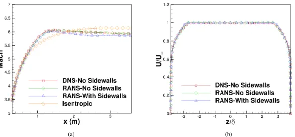
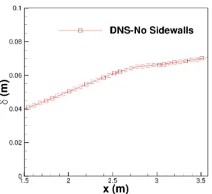
Mach number distribution between the DNS and RANS-No Sidewalls cases, although the RANS-With Sidewalls case indicates some noticeable differences over the downstream portion of the nozzle (x>1 m). These differences represent the effect of the side walls, especially as the thickness of the boundary layers increases significantly in the downstream region, and hence, is likely to influence the boundary layer development along the converging-diverging walls. The mean flow data has also been compared using the Mach number profiles at three different axial locations in the tunnel for the DNS-No Sidewalls and RANS-No Sidewalls cases. Figure 3 shows the favorable comparison between these flow fields when neither incorporates the effects of the side walls. The length of the boundary layer thickness along the nozzle wall has also been plotted as a function of the axial location in Figure 4 to show the growth of the turbulent boundary layer as the flow progresses through the tunnel.
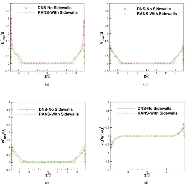
Figures 2b and 5 show the wall-normal distribution of the normalized streamwise velocity and Reynolds stresses, respectively, at an axial location ofx=3.3 m. For the RANS cases, the Reynolds stress components are calculated by using the Boussinesq approximation. The predictions for the mean velocity and Reynolds stresses match rather well between the DNS and the RANS results. Considering that the DNS domain, which consists of a section of the nozzle, is embedded within the RANS domain with the full-tunnel geometry, the favorable match between DNS and RANS results confirms that the tunnel nozzle flow is adequately reproduced with the DNS subdomain by using the inflow boundary conditions provided by the RANS.
Figure 6 shows that the rms pressure fluctuation field is nearly homogeneous outside the boundary layer, with a value of approximately 1.9% of the mean freestream pressure near the nozzle exit. The above value ofp0r ms/p∞outside
(a) (b)
Fig. 2 Comparison between Case DNS-No Sidewalls, Case RANS-No Sidewalls, and Case RANS-With Sidewalls. (a) Mach number distribution along the nozzle axis; (b) normalized streamwise velocity profile at x = 3.3 m. Mach number variation based on the isentropic approximation is also included in part (a) of the figure.
(a) (b) (c)
Fig. 3 Comparison between Case DNS-No Sidewalls and Case RANS-No Sidewalls. Mach number distribution along wall-normal distance at (a) x = 1 m; (b) x = 2 m; and (c) x = 3 m.
the nozzle-wall boundary layer (zw/δ> 1) is significantly higher than that induced by the turbulent boundary layer over a single flat plate at a similar freestream Mach number. This increase in the noise intensity is believed to be caused by the combined effect of acoustic radiation arriving from both the top and the bottom segments of the nozzle wall.
For both the nozzle flow and flow over flat plates, the DNS results show a similar frequency content of freestream pressure fluctuations (Fig. 7a). Figure 7b plots the bulk propagation speed of the pressure fluctuations as a function of wall-normal distance at a streamwise location ofx=3.3 m. The bulk propagation speed, (Ub), is defined as the value that minimized the difference between the real time evolution of p(x,t) and a frozen wave approximated by p(x-Ubt). The following expression is used to calculate the bulk propagation speed:
Ub =−
(∂p/∂t)(∂p/∂x)
∂p/∂x (1)
The wall-normal variation in bulk propagation speed is similar for all of the configurations in Figure 7b, but the flat plate cases reach higher peaks within the boundary layer before leveling out atUb ≈0.7U∞within the freestream region.
Fig. 4 Evolution of the boundary layer thickness as a function of streamwise location along the nozzle axis.
The propagation speed in the freestream region is nearly the same for both wind-tunnel and flat-plate configurations. The two-point correlation coefficient field in the streamwise wall-normal planes is defined by Eq. 2 as
Cp p(∆x,z,zr e f)= p0(x,y,z r e f,t)p0(x+∆x,y,z,t) (p02(x,y,z r e f,t))1/2(p02(x+∆x,y,z,t))1/2 (2)
where∆xdenotes spatial separation in the streamwise direction, andzr e f is the reference wall-normal location at which the correlation is computed. Figure 8 shows the contours of the two-point correlation coefficient for Case DNS-No Sidewalls atx=3.3 m and four different wall-normal locations (zr e f =0 m, 0.0688 m, 0.138 m, 0.251 m). At the wall (zr e f =0.251 m), the structure of pressure fluctuations is inclined almost perpendicular to the wall. In the freestream region away from the nozzle axis (zr e f =0.0688 m, 0.138 m), the correlation contours reveal downward-leaning structures inclined at a shallow angle with respect to the axis; the structures also indicate the dual origin of the acoustic field within a given cross-section of the nozzle, associated with the combined effect of acoustic radiation arriving from the top and bottom walls, respectively. At the nozzle axis (zr e f =0.251 m), the acoustic structures are almost symmetric about the axis and are mildly elongated along two separate directions associated with equal but opposite preferred orientations of the acoustic structures originating at the two walls.
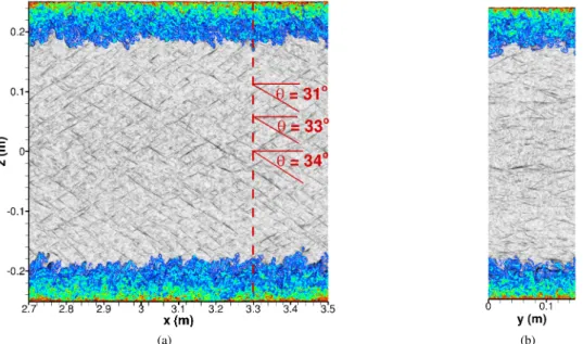
Figure 9 shows an instantaneous visualization of the density gradient associated with the radiated acoustic field. The prominent structures associated with acoustic fluctuations within the freestream region exhibit a preferred orientation of θ=32±2◦with respect to the nozzle centerline within the streamwise wall-normal plane. This inclination angle is similar to the Mach angle for the relative Mach numberMr (between the sources and free stream). The findings are consistent with the classic theory of “eddy Mach-wave radiation” and the early measurements of freestream noise by Laufer [3] during his unique wind tunnel experiments. Similar to the correlation contours in the∆x−zplane (Fig. 8), the density gradients reveal the dual origin of the acoustic field within a given cross-section of the nozzle, which adds to the stochastic nature of the wave front pattern at a given axial location.
IV. Summary
This paper has presented the RANS and DNS simulations of the nozzle-wall turbulent boundary layer in the NASA 20-Inch Mach 6 rectangular tunnel, along with an analysis of the freestream acoustic field within the core region of the nozzle. The properties of the nozzle wall boundary layer predicted by the DNS compare well with those estimated by Pate’s correlation and the RANS simulations with and without spanwise side-walls. The RANS and the DNS indicate good agreement in regard to streamwise variation in the freestream Mach number along the nozzle axis and the wall-normal profiles of mean velocity and Reynolds stresses near the nozzle exit. The observed agreement indicates that the tunnel nozzle flow is adequately reproduced with the DNS subdomain by using the inflow boundary conditions
(a) (b)
(c) (d)
Fig. 5 Comparison of Reynolds stresses at x = 3.3 m. (a)ur ms0 /uτ; (b)vr ms0 /uτ; (c)wr ms0 /uτ; (d) <u’w’>/u2τ;
provided by the RANS calculation. The frequency spectrum and bulk propagation speed of the acoustic disturbances match well between the DNS for the 2D nozzle configuration and the flat plate with a similar value of freestream Mach number. The two-point correlation of the pressure signal shows that the freestream acoustic structures consist of a superposition of downward-leaning inclined structures corresponding to a narrow range of orientations associated with acoustic radiation from either wall. As expected, the computed correlation contours are nearly symmetric about the flow direction at the nozzle exit. The prominent structures associated with acoustic fluctuations within the freestream region, as visualized by instantaneous density gradient, exhibit a preferred orientation similar to that predicted by the classic theory of “eddy Mach-wave radiation” and the early measurements of freestream noise by Laufer.
Future work will focus on further analysis of the acoustic field within the enclosed environment of the wind tunnel, as well as on the effect of tunnel side walls on the acoustic fluctuations.
Acknowledgments
Financial support for the work is being provided by NASA-EPSCoR Missouri and NASA Langley Research Center. Computational resources supporting this work were provided by the NASA High-End Computing (HEC) Program
(a) (b) (c)
Fig. 6 rms pressure fluctuation profile induced by the turbulent boundary layer over the nozzle wall of the NASA 20-in Mach 6 Tunnel (Case DNS-No Sidewalls). (a) Contours ofp0r ms/p∞inx−zplane; (b)pr ms0 /p∞as
a function of wall-normal coordinatezat selected streamwise locations; (c) comparison ofpr ms0 /p∞induced by
the turbulent boundary layer over the nozzle wall and three separate flat plate calculations at similar freestream Mach numbers [7, 27, 28]. znis the wall-normal distance.
(a) (b)
Fig. 7 Power spectral density and bulk propagation speed of freestream acoustic fluctuations induced by a turbulent boundary layer over the nozzle wall (Case DNS-No Sidewalls) and three separate flat plates at similar freestream Mach numbers [7, 27, 28]. z=0m corresponds to the center axis; znis the wall-normal distance;
the bulk propagation speed is defined according to Eq. 1.
through the NASA Advanced Supercomputing (NAS) Division at Ames Research Center. The authors would like to thank Jeffery White and Robert Baurle of NASA Langley Research Center for several technical discussions and their generous assistance with the RANS calculations for the nozzle.
References
[1] Fedorov, A. V., “Receptivity of a High-Speed Boundary Layer to Acoustic Disturbances,”Journal of Fluid Mechanics, Vol. 491, 2003, pp. 101–129.
[2] Zhong, X., and Wang, X., “Direct Numerical Simulation on the Receptivity, Instability, and Transition of Hypersonic Boundary Layers,”Annu. Rev. Fluid Mech., Vol. 44, 2012, pp. 527–561.
[3] Laufer, J., “Some Statistical Properties of the Pressure Field Radiated by a Turbulent Boundary Layer,”Physics of Fluids, Vol. 7, No. 8, 1964, pp. 1191–1197.
Fig. 8 Contours of constant streamwise wall-normal correlation coefficientCp p(∆x,z,zr e f) of the pressure
signal at multiple wall-normal locations (zr e f =0m,0.0688m,0.138m,0.251m) for Case DNS-No Sidewalls.
zr e f =0and0.251m are the nozzle axis and top nozzle wall, respectively; contours levels vary from0.2(blue)
to0.9(red) with increments of0.1.
(a) (b)
Fig. 9 Numerical schlieren images indicating density gradient contours associated with acoustic radiation in (a) streamwise plane (2.7< x<3.5m); (b) cross-sectional plane atx=3.3m. θis the inclination angle of the prominent structures associated with acoustic fluctuations within the freestream region; the vertical dashed line indicates the axial location of the selected cross section visualized in the right panel.
[4] Donaldson, J., and Coulter, S., “A Review of Free-Stream Flow Fluctuation and Steady-State Flow Quality Measurements in the AEDC/VKF Supersonic Tunnel A and Hypersonic Tunnel B,” AIAA Paper 95-6137, 1995.
[5] Schneider, S. P., “Effects of High-Speed Tunnel Noise on Laminar-Turbulent Transition,”Journal of Spacecraft and Rockets, Vol. 38, No. 3, 2001, pp. 323–333.
[6] Duan, L., Choudhari, M. M., and Wu, M., “Numerical Study of Pressure Fluctuations due to a Supersonic Turbulent Boundary Layer,”Journal of Fluid Mechanics, Vol. 746, 2014, pp. 165–192.
[7] Duan, L., Choudhari, M. M., and Zhang, C., “Pressure Fluctuations Induced by a Hypersonic Turbulent Boundary Layer,”
Journal of Fluid Mechanics, Vol. 804, 2016, pp. 578–607.
[8] Duan, L., and Choudhari, M. M., “Analysis of Numerical Simulation Database for Pressure Fluctuations Induced by High-Speed Turbulent Boundary Layers,” AIAA Paper 2014-2912, 2014.
[9] Duan, L., Choudhari, M. M., Chou, A., Munoz, F., Ali, S. R. C., Radespiel, R., Schilden, T., Schröder, W., Marineau, E. C., Casper, K. M., Chaudhry, R. S., Candler, G. V., Gray, K. A., Sweeney, C. J., and Schneider, S. P., “Characterization of Freestream Disturbances in Conventional Hypersonic Wind Tunnels,” AIAA Paper 2018-0347, 2018.
[10] Huang, J., Zhang, C., Duan, L., and Choudhari, M. M., “Direct Numerical Simulation of Hypersonic Turbulent Boundary Layers inside an Axisymmetric Nozzle,” AIAA Paper 2017-0067, 2017.
[11] Huang, J., L. Duan, L., and Choudhari, M. M., “Direct Numerical Simulation of Acoustic Noise Generation from the Nozzle Wall of a Hypersonic Wind Tunnel,” AIAA Paper 2017-3631, 2017.
[12] Baurle, R. A., and White, J. A., “Viscous Upwind Algorithm for Complex Flow Analysis,”Available: https://vulcan-cfd.larc.nasa.gov. Last accessed, Nov 3, 2017.
[13] Wu, M., and Martín, M. P., “Direct Numerical Simulation of Supersonic Boundary Layer over a Compression Ramp,”AIAA Journal, Vol. 45, No. 4, 2007, pp. 879–889.
[14] Jiang, G. S., and Shu, C. W., “Efficient Implementation of Weighted ENO Schemes,”Journal of Computational Physics, Vol. 126, No. 1, 1996, pp. 202–228.
[15] Taylor, E. M., Wu, M., and Martín, M. P., “Optimization of Nonlinear Error Sources for Weighted Non-Oscillatory Methods in Direct Numerical Simulations of Compressible Turbulence,”Journal of Computational Physics, Vol. 223, No. 1, 2006, pp. 384–397.
[16] Williamson, J., “Low-Storage Runge-Kutta Schemes,”Journal of Computational Physics, Vol. 35, No. 1, 1980, pp. 48–56. [17] Touber, E., and Sandham, N. D., “Oblique Shock Impinging on a Turbulent Boundary Layer: Low-Frequency Mechanisms,”
AIAA Paper 2008-4170, 2008.
[18] Dhamankar, N. S., Martha, C. S., Situ, Y., Aikens, K. M., Blaisdell, G. A., and Lyrintzis, A. S., “Digital Filter-Based Turbulent Inflow Generation for Jet Aeroacoustics on Non-Uniform Structured Grids,” AIAA Paper 2014-1401, 2014.
[19] Thompson, K. W., “Time Dependent Boundary Conditions for Hyperbolic Systems,”Journal of Computational Physics, Vol. 68, No. 1, 1987, pp. 1–24.
[20] Martín, M., “DNS of Hypersonic Turbulent Boundary Layers. Part I: Initialization and Comparison with Experiments,”Journal of Fluid Mechanics, Vol. 570, 2007, pp. 347–364.
[21] Duan, L., Beekman, I., and Martín, M. P., “Direct Numerical Simulation of Hypersonic Turbulent Boundary Layers. Part 3: Effect of Mach Number,”Journal of Fluid Mechanics, Vol. 672, 2011, pp. 245–267.
[22] Duan, L., Choudhari, M. M., Li, F., and Wu, M., “Direct Numerical Simulation of Transition in a Swept-Wing Boundary Layer,” AIAA Paper 2013-2617, 2013.
[23] Choudhari, M. M., Li, F., Duan, L., Chang, C.-L., Carpenter, M. H., Streett, C. L., and Malik, M. R., “Towards Bridging the Gaps in Holistic Transition Prediction via Numerical Simulations (Invited),” AIAA Paper 2013-2718, 2013.
[24] Pate, S. R., “Dominance of Radiated Aerodynamic Noise on Boundary-Layer Transition in Supersonic-Hypersonic Wind Tunnels,” Tech. rep., AEDC-TR-77-107, Arnold Engineering Development Center, 1978.
[25] Wood, N., “Calculation of the Turbulent Boundary Layer in the Nozzle of an Intermittent Axisymmetric Hypersonic Wind Tunnel,”Aeronautical Research Council C.P. No. 721, 1963.
[26] Smits, A. J., and Dussauge, J. P.,Turbulent Shear Layers in Supersonic Flow, 2nded., American Institute of Physics, 2006. [27] Zhang, C., Duan, L., and Choudhari, M. M., “Effect of Wall Cooling on Boundary Layer Induced Pressure Fluctuations at
Mach 6,”Journal of Fluid Mechanics, Vol. 822, 2017, pp. 5–30.
[28] Duan, L., Choudhari, M. M., Chou, A., Munoz, F., Ali, S. R. C., Radespiel, R., Schilden, T., Schröder, W., Marineau, E. C., Casper, K. M., Chaudhry, R. S., Candler, G. V., Gray, K. A., and Schneider, S. P., “Characterization of Freestream Disturbances in Conventional Hypersonic Wind Tunnels,”Journal of Spacecraft and Rockets, submitted, 2018.