Masters Theses Student Theses and Dissertations Summer 2015
Adjoint-based airfoil shape optimization in transonic flow
Adjoint-based airfoil shape optimization in transonic flow
Joe-Ray GramanziniFollow this and additional works at: https://scholarsmine.mst.edu/masters_theses Part of the Aerospace Engineering Commons
Department: Department:
Recommended Citation Recommended Citation
Gramanzini, Joe-Ray, "Adjoint-based airfoil shape optimization in transonic flow" (2015). Masters Theses. 7433.
https://scholarsmine.mst.edu/masters_theses/7433
This thesis is brought to you by Scholars' Mine, a service of the Missouri S&T Library and Learning Resources. This work is protected by U. S. Copyright Law. Unauthorized use including reproduction for redistribution requires the permission of the copyright holder. For more information, please contact [email protected].
by
JOE-RAY GRAMANZINI
A THESIS
Presented to the Faculty of the Graduate School of the MISSOURI UNIVERSITY OF SCIENCE AND TECHNOLOGY
in Partial Fulfillment of the Requirements for the Degree
MASTER OF SCIENCE IN AEROSPACE ENGINEERING
2015
Approved by
Dr. Serhat Hosder, Advisor Dr. David W. Riggins Dr. Kakkattukuzhy M. Isaac
ABSTRACT
The primary focus of this work is efficient aerodynamic shape optimization in transonic flow. Adjoint-based optimization techniques are employed on airfoil sections and evaluated in terms of computational accuracy as well as efficiency. This study examines two test cases proposed by the AIAA Aerodynamic Design Optimization Discussion Group. The first is a two-dimensional, transonic, inviscid, non-lifting optimization of a Modified-NACA 0012 airfoil. The second is a two-dimensional, transonic, viscous optimization problem using a RAE 2822 airfoil. The FUN3D CFD code of NASA Langley Research Center is used as the flow solver for the gradient-based optimization cases. Two shape parameterization techniques are employed to study their effect and the number of design variables on the final optimized shape: Multidisciplinary Aerodynamic-Structural Shape Optimization Using Deformation (MASSOUD) and the BandAids free-form deformation technique. For the two airfoil cases, angle of attack is treated as a global design variable. The thickness and camber distributions are the local design variables for MASSOUD, and selected airfoil surface grid points are the local design variables for BandAids. Using the MASSOUD technique, a drag reduction of 72.14% is achieved for the NACA 0012 case, reducing the total number of drag counts from 473.91 to 130.59. Employing the BandAids technique yields a 78.67% drag reduction, from 473.91 to 99.98. The RAE 2822 case exhibited a drag reduction from 217.79 to 132.79 counts, a 39.05% decrease using BandAids.
ACKNOWLEDGMENTS
I would like to sincerely thank my advisor Dr. Serhat Hosder for his guidance and expertise, and especially for providing me with this research opportunity. Thanks to him I have become a better student, researcher, and a better person. Thank you Dr. Hosder for all that you have done, I will never forget it. I would also like to thank my committee members, Dr. David Riggins and Dr. Kakkattukuzhy M. Isaac for their dedication, support, and time commitment to this research, as well as their contributions to my education. I would also like to thank the Department of Mechanical and Aerospace Engineering at the Missouri University of Science and Technology for the phenomenal educational and development opportunity, in addition to contributing funding for this research. I would also like to thank the NASA-Missouri Space Grant Consortium its funding toward this research. I further want to express my gratitude to my colleagues in the Aerospace Simulation Laboratory for all their help, guidance, and expertise. A special thanks goes to Harsheel Shah, Tom West, and Thomas Rehmeier. I would also like to thank my mother Olivia for always pushing me to be a better and stronger person each day. Finally I would like to thank, with all my love, my wife Sarah and my sons Giuseppe and Giovanni. I thank my wife for her understanding of my longing to further my education, and all of the pitfalls accompanying it. Sarah has been my best friend, greatest companion, and my greatest encouragement. I know that I might have not always been in the moment, but without your love and support I would have never pushed so hard and made it this far. I dedicate this degree to my wife and kids, for they have worked just as hard for it as I have.
TABLE OF CONTENTS
Page
ABSTRACT . . . iii
ACKNOWLEDGMENTS . . . iv
LIST OF ILLUSTRATIONS . . . vii
LIST OF TABLES . . . ix
NOMENCLATURE . . . x
SECTION 1. INTRODUCTION . . . 1
1.1. MOTIVATION FOR AERODYNAMIC SHAPE OPTIMIZATION . . . . 1
1.2. LITERATURE REVIEW . . . 2
1.3. OBJECTIVE AND CONTRIBUTION OF CURRENT STUDY . . . 4
1.4. THESIS OUTLINE . . . 4
2. COMPUTATIONAL TOOLS AND METHODOLOGY . . . 6
2.1. FLOW SOLVER . . . 6
2.1.1. Turbulence Model . . . 8
2.1.2. Boundary Conditions . . . 8
2.2. GEOMETRY AND COMPUTATIONAL GRIDS . . . 9
2.2.1. Modified-NACA 0012 . . . 9
2.2.2. RAE 2822 . . . 11
2.3. ADJOINT SOLVER. . . 14
3. OPTIMIZER AND SHAPE PARAMETERIZATION . . . 19
3.1. OPTIMIZER. . . 19
3.2. SHAPE PARAMETERIZATION . . . 20
3.3.1. Design Variables. . . 22
3.3.2. Design Variable Location . . . 25
3.4. BANDAIDS . . . 26
3.5. LINKING DESIGN VARIABLES . . . 29
4. OPTIMIZATION RESULTS FOR BENCHMARK PROBLEMS . . . 31
4.1. MODIFIED-NACA 0012 CASE . . . 31
4.2. RAE 2822 CASE . . . 37
5. CONCLUSIONS AND FUTURE WORK . . . 43
5.1. CONCLUSIONS . . . 43
5.2. FUTURE WORK . . . 44
APPENDICES A. FUN3D Nameless File . . . 45
B. MASSOUD Input File . . . 48
C. MASSOUD Input Generator . . . 51
D. BandAids Linking File . . . 56
E. Location of Design Variables . . . 58
BIBLIOGRAPHY . . . 60
LIST OF ILLUSTRATIONS
Figure Page
1.1: Design Iteration for Gradient-Based Optimization using Adjoint-Based
Sensitivities . . . 2
2.1: Boundary Conditions used in the Computations . . . 10
2.2: Computational Grid: Full Grid View . . . 12
2.3: Computational Grid: Airfoil View . . . 13
2.4: Grid Convergence Study for NACA 0012 case: Pressure Coefficient Distributions . . . 14
2.5: Mach Contour Plot for NACA 0012 at Grid Level 3 (Mach=0.85, α= 0.0) 15 2.6: Computational Grid: Full Grid View . . . 16
2.7: Computational Grid for RAE 2822 Airfoil: Close-up View . . . 17
2.8: Grid Convergence Study for NACA0012 case: Pressure Coefficient Distributions . . . 18
2.9: Mach Contour Plot at Grid level 3 (Mach=0.734, Re=6500000, α=2.978) 18 3.1: MASSOUD Process . . . 23
3.2: An example of the Baseline Coordinate System used in MASSOUD . . . 24
3.3: Deformation Coordinate System in MASSOUD . . . 25
3.4: Non-linear Global Deformation in MASSOUD . . . 25
3.5: BandAids Design Process . . . 28
3.6: Example Linking Control Points for MASSOUD . . . 30
4.1: Leading Edge Clustering of Design Variables using MASSOUD for the Modified-NACA 0012 . . . 33
4.2: Leading and Trailing Edge Clustering of Design Variables using MASSOUD for the Modified-NACA 0012 . . . 33
4.3: Design Variable Location using Bandaids for the Modified-NACA 0012 . . . 34
4.4: NACA Pressure Coefficient Plot Comparison . . . 36
4.6: Mach Contour of Optimized Shape with BandAids. . . 38 4.7: RAE 2822 Marking Surface . . . 39 4.8: Pressure Coefficient Plot Comparison between the RAE 2822 and
Optimized Shape . . . 41 4.9: Mach Contour Plot for the RAE 2822 profile optimized with BandAids . . . 42 4.10: RAE 2822 and Optimized Shape Comparison. . . 42
LIST OF TABLES
Table Page
2.1: Grid Convergence Results for NACA0012 Case . . . 11 2.2: Grid Convergence Results for the RAE2822 Case . . . 13 4.1: Summary of the Modified NACA0012 Parametric Design Study . . . 35 4.2: Grid Convergence of the Optimum Airfoil Shape obtained with BandAids
(NACA0012 Case) . . . 36 4.3: Optimal RAE 2822 Drag Results . . . 40 4.4: Grid Convergence of the Optimum Airfoil Shape obtained with BandAids
NOMENCLATURE
Symbol Description
M∞ Mach number
Mref Reference Mach number
Re Reynolds Number
Rref Reference Reynolds Number
u∗ Non-dimensionalized x-velocity v∗ Non-dimensionalized v-velocity x∗ Non-dimensionalized length x y∗ Non-dimensionalized length y P∗ Non-dimensionalized Pressure ρ∗ Non-dimensionalized Density T∗ Non-dimensionalized Temperature e∗ Non-dimensionalized internal energy µ∗ Non-dimensionalized viscosity
k Thermal Conductivity
Pr Prandtl Number
Y+ Dimensionless wall distance ∆s Wall distance
L Lagrange Function
D Design Variables
Q Flow Field Variables λf Costate of the Flow Field
R Discretized Residual Equation for Euler and Navier-Stokes Equations
f Objective function
uj Upper bound
j(x) Constraints
λ Lagrange Multiplier
g(x) Design Variables Pi Control points
p Degree of the Bernstein Polynomial
Wi Weight
R(v) Current Shape as a function of Design Variables δR Summation of perturbation
DV Design Variables SD Sensitivity Derivatives SOA Soft Object Algorithms
ξ Bivariate Coordinate η Bivariate Coordinate Z Thickness A Cross-Sectional Area LE Leading Edge T E Trailing Edge α Angle of Attack Cd Drag coefficient
Cdp Pressure Drag coefficient
CL Lift coefficient
CL∗ Desired profile lift coefficient value Cp Pressure coefficient
The following chapter outlines the subsequent research on aerodynamic shape optimization using computational fluid dynamics. First, motivation for aerodynamic shape optimization focusing on wing and airfoil configurations is given. Next, a literature review regarding parameterization and deformation techniques focusing on the airfoil geometries used in the current study is made. Then, the objectives of the study are explained followed by a description of the contributions to the area of aerodynamic shape optimization from this study. Lastly, an outline of the remainder of this thesis is provided.
1.1. MOTIVATION FOR AERODYNAMIC SHAPE OPTIMIZATION The wing is one of the most crucial components of aircraft design, due to its function of sustaining lift, and storage of the fuel. This alone constrains the design engineer and must be optimized between aerodynamic performance, range and endurance of the aircraft. With the rise of fuel prices, drag reduction techniques are playing a critical role in the design process. The reduction of drag can be obtained by incorporating a better design, through optimizing the shape. In the past this could be done by well-experience aerodynamicist and experimentation, which is an expensive procedure that could result in a configuration that may have a reduction in drag, but may not meet other conditions required such as lift or pitch. The computational method is the second option, which allows an efficient and robust design to be achieved. This method also allows the designer to modify an existing geometry that will meet the extensive constraints for a given flight condition.
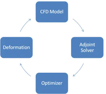
The first procedure of shape optimization is to parameterize the geometry, which is done to define the shape in terms of design variables. The parameterization of the
geometry is only needed to be done once at the start of the design process. To conduct shape optimization, there consists four subroutines for each design iteration, presented in Figure 1.1. The first step of the aerodynamic shape optimization design cycle is to solve for the fluid flow using a computational fluid dynamics solver. The second step is to determine the gradients of the objective function in relation to the design variables using the adjoint solver. The gradients calculated from the adjoint are then fed into the optimization algorithm. The final step for each iteration is the deformation of the computational domain. The design cycle is an iterative process which stops only if the solution can not be improved any further or an optimal solution is obtained.
Figure 1.1: Design Iteration for Gradient-Based Optimization using Adjoint-Based Sensitivities
1.2. LITERATURE REVIEW
In recent years an increasing amount of research has gone into gradient-based aerodynamic shape optimization of airfoils. The biggest challenge with aerodynamic
shape optimization is the variety of parameterization techniques, optimization algorithm, determining the sensitivity derivatives, and the efficiency and accuracy of the design process. To calculate the sensitivity derivatives there are currently two predominate methods, the first is the finite difference approach. This approach is great for simple design cases since it is efficient for a small number of design variables. However this method is not ideal if the number of design variables are relativity large, making this method suitable for airfoils design optimization with only a few design variables, but not so much for general airfoils or wing optimization since the number of design variables can be quite large for theses cases. The adjoint method is an alternative technique commonly used to determine the sensitivity derivatives, which was first implemented in aerodynamic design by Antony Jameson [1]. Jameson et. al developed the adjoint solver for both the Euler [2] and Navier-Stokes equations [3]. Nielson and Anderson [4] applied this technique into an unstructured Navier-Stokes solver.
Recently the AIAA Aerodynamic Shape Optimization Design Group [5] released a series of design cases, which resulted in a variety of parameterization techniques and optimization algorithms explored. For the study of the modified-NACA 0012 and RAE 2822 Leifsson et al [6] implemented a PARSEC method by using twelve parameters to define the control points and FLUENT [7] as the flow solver. Tesfahunegn et al.[8] applied a surrogate-based optimization technique, which was done for computational cost reduction. For the modified-NACA 0012, Tesfahunegn [8] was able to achieve a drag reduction of 281.5 counts, and for the RAE 2822 case a reduction of 38.2 drag counts. The most popular method of calculating the sensitivity derivatives for these cases involved the use of the adjoint solver. Telidetzki [9], utilized the B-spline volumes to parameterize the modified-NACA 0012, with a sparse sequential quadratic programming (SNOPT) optimizer, using Jetstream as the flow solver and the adjoint solver to calculate the sensitivity derivatives. Telidetzki
[9] was able to produce a drag reduction of 40.35 counts for the modified-NACA 0012. Similar to the work presented in this thesis, Amoignon [10] conducted a comparison of parameterization, the first a trivariate free form deformation and the second a Radial Basis Function (RBF) approach. Amoignon [10] used a unstructured flow solver, Edge, with a sequential quadratic programming (SQP) optimizer for both cases, and a finite difference method to calculate the sensitivity derivatives. A drag reduction of 361.2 drag counts was achieved for the modified-NACA 0012 using free-form defree-formation (FFD). Using both FFD and RBF, Amoignon was able to get a drag reduction of 68 and 78 drag counts respectively for the RAE 2822. In another study, Carrier [11] used a Bezier-curve technique to parameterize the modified-NACA 0012 and RAE 2822. Carrier [11] used a structured CFD solver developed by ONERA, elsA, and an adjoint solver to calculate the sensitivity derivatives. The optimization algorithm used by Carrier [11] was a Flecher Reeves [12] conjugate gradient optimizer. Carrier [11] obtained a reduction of 387.1 drag counts for the modified-NACA 0012 and 91.4 drag counts for the RAE 2822.
1.3. OBJECTIVE AND CONTRIBUTION OF CURRENT STUDY The primary objective of this thesis is to perform adjoint-based optimization on two airfoil cases taken from AIAA Aerodynamic Shape Optimization Group [5] in the transonic flow regime using FUN3D [13]. The first contribution of this study is to perform a comparison between two shape parameterization techniques. The first technique is a multidisciplinary parameterization tool known as MASSOUD [14], the second is a modified free form deformation method call BandAids [15]. The second contribution is to determine the optimal number of control points for both methods.
1.4. THESIS OUTLINE
computational models and the methodologies used. This includes an explanation of the computational fluid dynamics code and adjoint solver, solution methodology, boundary conditions and the turbulence model used. Furthermore, generation of the computational mesh, and the grid convergence is presented.
Section 3 outlines the optimization tools including the optimizer and the two shape parametrization techniques. The first parameterization tool uses aerodynamic shape characteristics such as planform and thickness to parameterize the geometry. The second method uses a bivariate free-form deformation technique, by marking grid points along the surface as design variables.
Section 4 outlines the results of two optimization cases defined by the AIAA Aerodynamic Shape Optimization Group [5]: the first case involves the optimization of a non-lifting airfoil in transonic, inviscid flow airfoil, using MASSOUD and BandAids. The second case is the optimization of a supercritical airfoil in transonic, viscous flow using BandAids.
In the last section, a conclusion is given to summarize the optimized geometries and a comparison to the original shape. Following the conclusions, suggestions for future work are given. The setup procedure for running the flow solver and optimization is given in the Appendices.
2. COMPUTATIONAL TOOLS AND METHODOLOGY
This section outlines the computational models utilized for this study and includes a description of the flow solver, computational grids and grid convergence, and adjoint solver used for the modified-NACA 0012 and RAE 2822 airfoils.
2.1. FLOW SOLVER
The computational fluid dynamics (CFD) flow solver used in this study was the Fully Unstructured Navier-Stokes 3-D (FUN3D) [13] code from NASA Langley Research Center. FUN3D is an unstructured node-based solver which uses a finite volume scheme with a second order spatial discretization. The selection of FUN3D was based on its effectiveness to solve a variety of flow regime problems, in addition to the code having a built in design component. The flow solver is designed with a diversity of flux schemes and limiters, with the potential to freeze the limiter at a designated iteration, giving the user full control of the solver.
Solutions for the inviscid flow cases used a two-dimensional steady-state non-dimensional compressible form of Euler Equations, given in Equations 1,2,3 and 4. Here Equation 1 is the conservation of mass, Equation 2 and 3 are the momentum equation in the x and y directions respectively, and Equation 4 is the conservation of energy. ∂(ρ∗u∗) ∂x∗ + ∂(ρ∗v∗) ∂y∗ = 0 (1) ∂ ∂x∗[ρ ∗ u∗2 +P∗] +∂(ρ ∗u∗v∗) ∂y∗ = 0 (2) ∂ ∂y∗[ρ ∗ v∗2+P∗] +∂(ρ ∗u∗v∗) ∂x∗ = 0 (3) ∂ ∂x∗[(e ∗ +P∗)u∗] + ∂ ∂y∗[(e ∗ +P∗)v∗] = 0 (4)
Here, u∗, and v∗ are the velocity component in the x and y direction, ρ∗ is the
fluid density, P∗ is the pressure, and e∗ is the internal energy. Note the asterisk (*) corresponds to a non-dimensional quantity. For the Modified-NACA 0012 airfoil case, a Van Leer Flux vector splitting scheme [16] was used for the inviscid flux construction, with a hvanleer flux limiter, a stencil-based Van Leer limiter [17] augmented with a heuristic pressure limiter [18]. The limiter improved the convergence of the flow solver in the presence of solution continuities such as shock waves, with the capability of freezing the limiter, while providing an exact linearization required for the adjoint convergence [18].
To solve the viscous flow cases, the two-dimensional steady-state compressible formulation of non-dimensionalized Navier-Stokes equations were used. The equation that are numerically solved by FUN3D are shown in Equations 5, 6, 7, and 8 which are the conservation equations for mass, momentum equation in the x and y directions, and energy respectively for a two-dimensional flow.
∂(ρ∗u∗) ∂x∗ + ∂(ρ∗v∗) ∂y∗ = 0 (5) ∂(ρ∗u∗2) ∂x∗ + ∂(ρ∗u∗v∗) ∂y∗ + ∂P∗ ∂x∗ − Mref ReLref µ 2 3 2∂u ∗ ∂x∗ − ∂v∗ ∂y∗ ∂u∗ ∂y∗ + ∂v∗ ∂x∗ = 0 (6) ∂(ρ∗v∗2) ∂y∗ + ∂(ρ∗u∗v∗) ∂x∗ + ∂P∗ ∂y∗ − Mref ReLref µ 2 3 2∂v ∗ ∂y∗ − ∂u∗ ∂x∗ ∂u∗ ∂y∗ + ∂v∗ ∂x∗ = 0 (7) ∂ ∂x∗ (e∗+P∗)u∗− Mref ReLref µ∗ 2u∗ 3 2∂u ∗ ∂x∗ − ∂v∗ ∂y∗ +v ∂u∗ ∂y∗ + ∂v∗ ∂x∗ − 1 Pr(γ−1) ∂T ∂x + ∂ ∂y∗ (e∗+P∗)v∗− Mref ReLref µ∗ 2v∗ 3 2 ∂v ∗ ∂yx∗ − ∂u∗ ∂x∗ +u ∂u∗ ∂y∗ + ∂v∗ ∂x∗ − 1 Pr(γ−1) ∂T ∂y = 0 (8)
Here, µ* is the viscosity, γ is the ratio of specific heats, P r is the Prandtl Number which is defined in Equation 9, Mref and Rref are the Mach number and
Reynolds Number respectively. Note that the subscript ref denotes to the reference quantities, which correspond to free-stream conditions. In Equation 9 k is the thermal conductivity of the fluid flow.
P r= Cpµ
k (9)
For the viscous flow simulations, the Navier-Stokes equations were solved by using a 2nd Order upwind Roe Flux difference splitting scheme [19]. The hMinMod limiter,
a stencil-based MinMod limiter [20] with a heuristic pressure limiter augmentation [18], was selected as the flux limiter. The limiter was selected due to the capability of freezing the limiter in both the adjoint and flow solver. This limiter reduces the reconstruction gradient in the location of high pressure gradients. This modification defines a thin width for the discontinuity [18]. The convergence criteria for Navier-Stokes equations was set to 10−12 in terms of the convergence of the L2 norm of each
equation, while the convergence requirements for the adjoint solver was set to 10−8.
2.1.1. Turbulence Model. All viscous simulations presented in this work used the Spalart-Allmaras (SA) turbulence model [21], a one-equation eddy viscosity model used for modeling the turbulence in fluid flows. The SA model was used due to its proven level of robustness in a plethora of problems especially in the transonic flow regime. The Spalart-Allmaras was non-dimensionalized by the same quantities as the flow solver above, resulting in the following Equation 10 for a fully turbulent flow [22]: D˜v Dt = M∞ σRe ∇ ·[(v + (1 +cb2)˜v)∇v˜]−cb2v˜∇ 2v˜ −M∞ Re cw1fw− cb1 κ2ft2 ˜ v d 2 +cb1(1−ft2) ˜Sv˜+ Re M∞ft1∇U 2 (10)
For further details about the SA model, and the integration into FUN3D, the reader should refer to references [21] and [22]
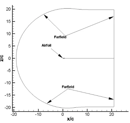
boundary conditions, shown in Figure 2.1. The outer boundaries were set to Riemann invariant farfield boundary condition. The surface of the modified-NACA 0012 was set to a tangency boundary condition, which sets a zero normal velocity at the surface. The RAE 2822 airfoil surface was set to a viscous boundary condition, which imposes a no-slip condition on the solid surface. Since FUN3D is a three dimensional flow solver, each side boundary was set to a symmetry plane, which enforces symmetry at the y Cartesian plane.
The modified-NACA 0012 farfield boundary condition was set with a free-stream Mach number of 0.85 with an angle of attack of 0.0 degrees. The RAE 2822 farfield boundary condition was set with a free-stream Mach number of 0.734, with an angle of attack of 2.97 degrees for the level 3 grid. Each grid level for the RAE 2822 varied in angle of attack to match the lift constraint of (CL= 0.824) required. The Reynolds
number per unit length was set to 6,500,000. Lastly the Prandtl number of the fluid flow was set to 0.72.
2.2. GEOMETRY AND COMPUTATIONAL GRIDS
2.2.1. Modified-NACA 0012. The first geometry consisted of a symmetric modified-NACA 0012 airfoil, with a chord length of 1 grid unit, where x ∈ [0,1].
The modified-NACA 0012 airfoil was defined by a 4th order B´ezier curve given with Equation 11, specified by the AIAA Aerodynamic Design Group. This modification to NACA 0012 geometry resulted in a trailing edge with zero thickness.
z =±0.6(0.2969√x−0.1260x−0.3516x2+ 0.2843x3−0.1036x4) (11)
To produce the surface grid points, a simple MATLAB script was created to generate 200 points for the upper and lower surface, to allow a smooth rendering of the geometry. The computational domain was created using a hyperbolic
C-Figure 2.1: Boundary Conditions used in the Computations
mesh grid generator [23], HYGRID for short. The HYGRID generator is limited to structured mesh generation. In order to implement an unstructured mesh into FUN3D, the y-symmetry boundary was converted to a unstructured domain, using the diagonalization tool. Once the unstructured domain was created a translational extrusion was conducted 1 grid unit in the y-direction, using the Pointwise Meshing Software [24].
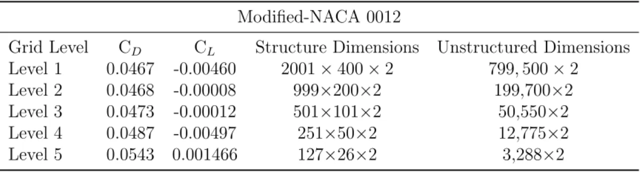
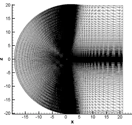
A grid convergence study was conducted in order to determine the optimal mesh size. Five grid levels were produced to show grid independence. Table 2.1 depicts the grid size for each grid level as well as numerical results from the study. Each grid level consisted of a grid size of 20 chord lengths from the surface of the airfoil. The baseline mesh, grid level 3, consisted of a wall spacing of 0.002 grid units normal to
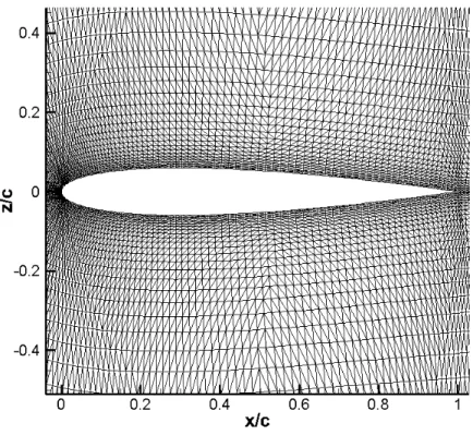
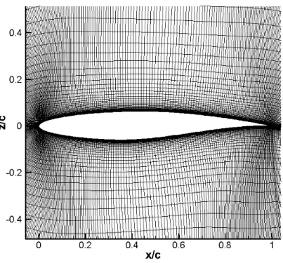
the surface of the modified-NACA 0012. The dimension of the baseline grid used was 50,550x2 grid points. Figure 2.2 depicts the baseline unstructured computational grid for the modified-NACA 0012. The computational grid near the surface of the modified-NACA 0012, is presented in Figure 2.3. From the examination of Table 2.1,
Table 2.1: Grid Convergence Results for NACA0012 Case Modified-NACA 0012
Grid Level CD CL Structure Dimensions Unstructured Dimensions
Level 1 0.0467 -0.00460 2001×400×2 799,500×2
Level 2 0.0468 -0.00008 999×200×2 199,700×2
Level 3 0.0473 -0.00012 501×101×2 50,550×2
Level 4 0.0487 -0.00497 251×50×2 12,775×2
Level 5 0.0543 0.001466 127×26×2 3,288×2
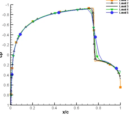
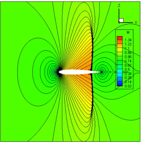
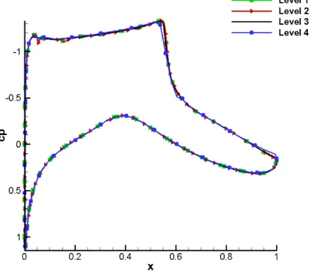
it can seen that there is a difference of 1.0 drag count between the first and second grid levels. To insure a low computational time Level 3 was selected as the baseline grid with a difference of 5 drag counts from level 2. The pressure coefficient plots for all of the modified-NACA 0012 grid levels,shown in Figure 2.4, shows a slight deviation between grid levels 1,through 3. The deviation occurs at the location of the shock. From the small perturbation in the coefficient of pressure plot and the small variation in drag counts, level 3 was determined to be suitable grid for the design procedure. Presented in Figure 2.5, is the Mach contour for the baseline mesh which the presence of a strong stock is evident.
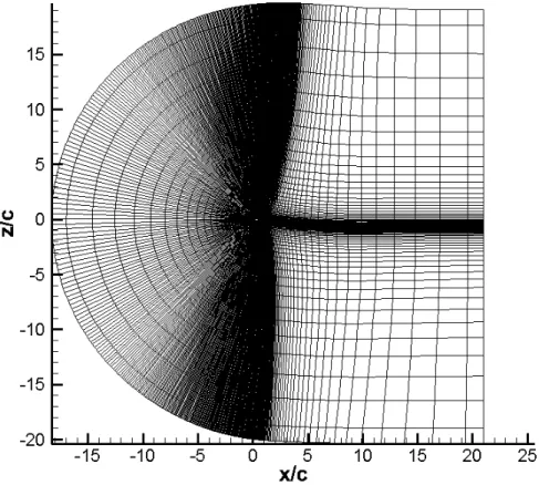
2.2.2. RAE 2822. The second case examined a RAE 2822 airfoil, with chord length of 1 grid unit. The RAE 2822 geometry was obtain from UIUC Airfoil Data Site [25]. To produce a smooth upper and lower surface, a cubic-spline technique was used to increase the number of points from 65 to 200 for both surfaces. The
Figure 2.2: Computational Grid: Full Grid View
computational grid, shown in figure 2.4, was created using HYGRID, no modification to the element type was conducted for the RAE2822 domains.
As with the modified-NACA 0012 case, a grid convergence study was conducted for the RAE 2822 grid. Three additional grid levels where created, one grid level lower and two grid levels higher then the original mesh, shown in Table 2.2. Each grid level had a dimension of 20 chord lengths from the surface of the RAE 2822. It is demonstrated in Table 2.2 and Figure 2.8, that there is no significance deference between grid level 2 and 3. To minimize computational time, grid level 3 was selected as the baseline grid. Grid level 3 has a dimension of 501x101x2, with a wall spacing (∆S) normal to the surface of 1.05x10⁻⁶ grid units, which corresponding to a Y+ of 0.250. The computational domain of grid level 3 for the RAE2822 is shown in Figure
Figure 2.3: Computational Grid: Airfoil View
Table 2.2: Grid Convergence Results for the RAE2822 Case RAE 2822
Grid Level CD CL Structure Dimensions α ∆S Y+
Level 1 214.447 0.8240 2000×400×2 2.958 0.00000024 0.063 Level 2 214.588 0.8240 999×200×2 2.950 0.00000050 0.125 Level 3 216.815 0.8240 501×101×2 2.970 0.00000105 0.250 Level 4 236.233 0.8240 251×50×2 3.090 0.00000212 0.500
2.6, with a focused airfoil view in Figure 2.7. Presented in Figure 2.9, the Mach contour of the baseline mesh of the RAE 2822 at a corrected angle of attack of 2.978.
Figure 2.4: Grid Convergence Study for NACA 0012 case: Pressure Coefficient Distributions
2.3. ADJOINT SOLVER
In this current work, a gradient-based non-linear constraint optimization approach was used, which utilized the FUN3D code to obtain the solution to flow field and discrete-adjoint equations. The design sensitivity derivatives (the gradients) used in the optimization were obtained from the solution of adjoint equations.
A Lagrange Function, L, is defined by the objective function and adjoint variables in the design approach, given in Equation 12
Figure 2.5: Mach Contour Plot for NACA 0012 at Grid Level 3 (Mach=0.85,α= 0.0)
Here f(D,Q,X) is the objective function to be minimized, and Λf is the costate
variable, or the vector of Lagrange multiplier, for the flow field. R is the discretized residual equations for either the steady-state Navier-Stokes or Euler equations. The discretized residuals are a function of the design variables (D), X represents the computational grid, and the flowfield variables (Q) [26]. To derive the discrete Adjoint formulation, the flow field adjoint equation is differentiated with respect to the design variables, D, which yields the following Equation 13.
dL dD = ∂f ∂D + ∂X ∂D T ∂f ∂X + ∂Q ∂D T ∂f ∂Q + ∂R ∂Q T Λf + ∂R ∂D T + ∂X ∂D T ∂R ∂X T Λf (13)
Figure 2.6: Computational Grid: Full Grid View
Since the costate variable, Λf, is essentially arbitrary, the terms multiplied by∂Q/∂D
can be eliminated by Equation 14[4].
∂R ∂Q T Λf =− ∂f ∂Q (14)
The above expression represents the discrete adjoint equation for the flow field used for the optimization procedure. In order to determine the sensitivity derivatives, the flow field variables must first be calculated. Once Q is determined the Lagrange multipliers, Λf, is calculated by the adjoint solver in an iterative process[4]. Once the
Figure 2.7: Computational Grid for RAE 2822 Airfoil: Close-up View
be obtained by solving a single matrix vector product of the following equation:
∂L ∂D = ∂f ∂D + ∂X ∂D T ∂f ∂X + ∂R ∂D T + ∂X ∂D T ∂X ∂D T Λf (15)
Once the sensitivity derivatives are determined, the next step is the optimization and deformation of the aerodynamic shape. This will be discussed in the following section.
Figure 2.8: Grid Convergence Study for NACA0012 case: Pressure Coefficient Distributions
3. OPTIMIZER AND SHAPE PARAMETERIZATION
This section discusses the optimizer, shape, parameterization, and deformation techniques used in the current study. The first parameterization tool discussed will be MASSOUD, which uses a modification to the deformation algorithms discussed by Samareh [14] [27]. This technique allows the design variables of the optimization process to be defined as aerodynamic geometry characteristics. A discussion of how Samareh [14] uses a combination of parameterization techniques to form MASSOUD will be discussed as well. The second parameterization technique discussed in this section will be a free-form deformation tool, BandAids. This method compresses a trivariate volume deformation technique to a bivariate surface deformation, which eliminates the number of design variables needed to define the design space by an order of magnitude.
3.1. OPTIMIZER
The NPSOL [28] code, which is based on a sequential quadratic programming (SQP) optimization algorithm was implemented as the optimizer in the current study. The optimizer has the capability to minimize smooth functions with either linear and nonlinear constraints, making the algorithm perfect for aerodynamic shape optimization problems. For NPSOL to solve the objective function subjected to given constraints, the problem must formulated as follows:
minimize
xεR
f(x)
subject to lj ≤r(x)≤uj
Here f(x) is the objective (cost) function to be minimized, x is the set of design variables, and r(x) are the constraints for the design. For the optimization process
all constraint and design variables must be set with an upper and lower bound. If equality constraints are desired the constraint must be specified as uj =lj.
NPSOL uses the gradients of the objective function with respect to the design variables, g(x), and the Jacobian of the constraints to solve for the vector of the Lagrange multipliers λ, such that equation (16) is zero. This determines a feasible point to satisfy the first order condition for optimality.
g(x) = J(x)Tλ (16)
In NPSOL, the search direction is computed from the solution of a Quadratic Program (QP) sub-problem. Once the search direction is determined; the step length is computed by a Lagrangian merit function. A quasi-Newton update is then used to update the Hessian of the Lagrangian. This process is repeated until a local minimum is achieved. The reader should refer to Reference [28] for more details on the optimization algorithm and the NPSOL code.
3.2. SHAPE PARAMETERIZATION
In order to perform aerodynamic shape optimization, the geometry must be expressed by a finite number of variables, known as shape parameterization, since for aerodynamics shapes a detail parameterization of the skin, outer mold line (OML), of the airfoil or wing is needed. There are eight parameterization techniques [29] available to identify the design variables.
The polynomial and spline parameterization technique is a common method used for optimization. This method better maps the curvature of the geometry, with fewer number of control points then most methods. For simple curves the polynomial approach using a power basis form, but this method is prone to error if the curve is moderately complex. If the curve is complex then the use of a Bezier Curve can
be implicated for parameterization. A single nth order Bezier curve is modeled in
Equation (17), where n is the number of control points (design variables), Bi,p(u)
are the degree p of the Bernstein polynomials, and Pi are the control points. Once
the control points are determined these can be used as the design variables for the optimization process. ¯ Rg(u) = n X i−1 ¯ PiBi,p(u) (17)
The Bezier curve formulation is ideal for the optimization of simple aerodynamic shape, as the complexity of the shape increases the number of design variables and the degree of the Bernstein polynomial to accurately represent the surface increase, which can result in wiggles in the surface geometry. A solution to this is to use multiple Bezier curves, known as B-Splines shown in Equation 18, to define the complex curve. Here ¯P are the B-spline control points, p is the degree, and Ni,j(u) is the B-spline
basis function. ¯ Rg(u) = n X i−1 ¯ PiNi,p(u) (18)
B-splines provide a near perfect representation of the curve, with great shape control of the deformation, since the control points only have a local zone of influence. The only drawback to B-Splines is that it can not handle conic sections accurately [29]. To account for this, a special formulation of the B-Spline known as the Non-Uniform Rational B-Splines(NURBS) are developed. The following gives the equations for the NURBS, where Wi are the weights.
¯ R(u) = n P i−1 ¯ PiWiNi,p(u) n P i−1 Ni,p(u)Wi (19) 3.3. MASSOUD
a curve to define a geometry relative to the design variables. Multidisciplinary Aerodynamic-Structural Shape Optimization Using Deformation[14] (MASSOUD) is a parameterization approach used for both simple and complex aerodynamic shapes. This technique is compatible to be used with either low and high fidelity computational fluid dynamics simulations. The MASSOUD process at each design iteration is depicted in Figure 3.1. The MASSOUD technique differs from the typical Multidisciplinary Shape Optimization (MSO) process since it uses a meshed based parameterization technique, which allows the parameterization to be independent of of grid topology, eliminating the need for mesh regeneration after each design cycle. This is accomplished by parameterization of shape perturbations, rather then the shape itself, limiting MASSOUD to small changes in the shape, which in-turn decrease the number of design variables needed for parameterization. Through out the optimization design cycle, the geometry and computational grid is updated by the relation given in Equation 20:
¯
R(¯v) = ¯r+ ∆ ¯R(¯v) (20)
¯
R(¯v) is the current shape as a function of the design variables (¯v), ¯r is the baseline shape, and ∆ ¯R(¯v) is the shape perturbation [14]. ∆ ¯R(¯v) can be interpreted as a summation of how the geometry is parameterized. For MASSOUD, this corresponds to the parametrization of the geometry in terms of thickness, camber, twist, shear, and planform.
3.3.1. Design Variables. A design variable is a controllable point in a design space in which the design engineer can specify. MASSOUD, unlike other parameterization tools, is tailored for aerodynamic shapes as it parameterizes the perturbation of geometry with respect to thickness, camber, twist, dihedral, and/or planform. This is possible through the use of a modification to the Soft-Object
Figure 3.1: MASSOUD Process
Animation (SOA) algorithms. The SOA algorithms are used in computer animation graphics to define environmentally interactive shapes with the ability to twist and bend freely. Samareh [15] was able to modify the SOA algorithms in four main steps. First, selecting the deformation technique and defining the forward mapping from the deformation coordinate system to the baseline grid coordinate system. Second, establishing a backward mapping from the baseline grid to the deformation coordinate system, and fixing the mapping parameters as to make it independent of shape perturbation. Third, perturbing the design variables, and finally, evaluating the grid perturbation and shape sensitivity derivatives.
MASSOUD uses a combination of Non-Uniform Rational B-splines and properties of the National Advisory Committee for Aeronautics (NACA) airfoil series to parameterize shape perturbation as a function of thickness and camber. This is done to retain the smoothness of the initial geometry. The definition of the perturbation of the grid as well as the forward mapping for thickness and camber are given by Equation 21 and 22 respectively, an example of the baseline coordinate
system is shown in Figure 3.2. δR¯th = I P i=0 Ni,p(ξ) J P j=0 Nj,q(η)Wi,j(P¯)thi,j I P i=0 Ni,p(ξ) J P j=0 Nj,q(η)Wi,j (21) δR¯ca = I P i=0 Ni,p(ξ) J P j=0 Nj,q(η)Wi,j(P¯)cai,j I P i=0 Ni,p(ξ) J P j=0 Nj,q(η)Wi,j (22)
The backward mapping was conducted by using the percentage of the chord for ξ direction and using the span location y for η. Figure 3.3 shows the deformed coordinate system. Once the design variables are perturbed, a shape sensitivity derivative is needed to evaluate the grid perturbation. The equations used for parameterization of thickness and camber are also used to calculate the sensitivity derivatives for the respective design variables. Since this portion of the MASSOUD uses a spline parameterization technique, the sensitivity derivatives are only calculated at the beginning of each design iteration. The second embedded
Figure 3.3: Deformation Coordinate System in MASSOUD
parameterization method in MASSOUD is the nonlinear global deformation technique, which is used for the twist and shear (dihedral) design variables. This technique uses modification to the soft object animation algorithms discussed by Barr [30]. The design variable for twist defines the twisting angle as the difference between the incidence angle at the root and the incidence angle of the airfoil section at the twist location. The polyhedral sections are defined by the difference between the z coordinate at the leading edge of the root and the z coordinate of leading edge of the airfoil section at the shear design location. The deformation of the two design variables are modified by a twist cylinder[14], which can deform the section of the wing only in the twist plane, as shown in Figure 3.4.
3.3.2. Design Variable Location. A parametric study was conducted to determine the number of control points needed to find the optimal solution. To
eliminate arbitrary placing of control points along the surface, Equation 23 was used to create a consistent distribution pattern as the number of control points is increased.
xi = 1−cos(θi) (23)
Here xi is the location of each control point, at a specified design angleθi. The design
angle was calculated by dividing a initial angle of 90 degrees by the desired number of control points increased by one, this allowed the angle for each control point to be the increased by same amount. In MASSOUD the user must specify the control point location as a non-dimensional value of the chord length. The initial angle was selected to bound the control points between zero and one. The above distribution equation allowed for clustering at both the leading edge and trailing edge of the airfoil section. By dividing the previous equation by two, Equation 24, this leads to clustering of control points only at the leading edge of the airfoil.
xi =
1−cos(θi)
2 (24)
An implementation of both equations for ten control points can be found in the Appendix E. MASSOUD was only able to be used with the modified-NACA 0012 case in this study. Due to the highly cambered shape of the RAE 2822, a kink occurred at the trailing edge, during the optimization process that could not be resolved. This is a known issue with the MASSOUD code as confirmed by the NASA researchers.
3.4. BANDAIDS
The second shape parametrization method used in the current study is BandAids, which is based on the free form deformation technique. Introduced by Barr [30], a model was developed to obtain realistic shapes from a physical iteration. This treated the shape like rubber, allow it to bend, compress, expand and twist without
degrading the topology. The deformation is handed by using the grid points that define the shape as control point. With modification from Sederberg and Parry [31], the deformation method operated in the whole space, defining a trivariate volume. The trivariate FFD uses either NURBS or B-splines to define a marking box that encompasses the geometric shape for deformation. The advantage of this technique is that it can be applied to any shape, and maintain the topology of the grid. The only pitfall to this parameterization technique is to the designer, there are no physical representation where to place the control points, making it difficult to set geometric constraints.
Samareh [15] was able to modify the classical FFD and reduce the number of design variables by an order of magnitude by compressing the ξ axis. This allowed the marking to be applied directly to the geometry, while maintaining grid topology, resulting in better control of the geometry changes [15]. An advantage of using BandAids is the ability to perform medium and small shape perturbations, which is important as large perturbation can result in a poor grid topology. This technique parameterizes the perturbation in the surface of the grid, rather than the shape, and produces a fix topology through the optimization process. Since the topology is fixed, during the design iterations the grid is deformed and regenerated automatically [15]. The interactive design process for BandAids is depicted in Figure 3.5.
The BandAids parametrization process is composed of three steps. The first is to define the design region with the use of a marking surface. The marking surface projects a series NURBS onto the outer mold line (OML) of the geometry using the surface grid points as design variables. This parameterization technique is ideal for complex non-aerodynamic geometries or sections of the aircraft where the fuselage and wing are joined, such as fillets. There are two conditions that must be satisfied when using marking surfaces. First no marking surface can intersect or overlap any other marking surface. This is not true for the geometry, a marking surface may
Figure 3.5: BandAids Design Process
cross the geometry if needed. The second condition is that the marking surface must lie within a specified tolerance from the design region. The final two steps in the BandAids process are handled internally. The second step projects the grid points onto the marking surface, by linking the surface grid point to closest marking surface [15] and creating a bivariate coordinate system (ξ, η). Since the marking surface and grid points are linked, as the marking surface is perturbed the grid points on the shape are perturbed with the same magnitude and direction of the marking surface. This is due to the inverse mapping between the deformation and baseline coordinate system [15]. The final step is to define the NURBS for the design surface, shown in Equation 25, where ∆r are the NURBS, and Cm are the products of the B-spline
basis functions. ∆rn(v) = ∆r(v, ξn, ηn) = M X m Cm(ξn, ηn)vm (25)
Analytical sensitivity derivatives of grid points with respect to design variables are determined using the following Equation:
∂rn(v)
∂vm
= ∂(∆rn(v)) ∂vm
=Cm(ξn, ηn) (26)
The grid point sensitivity shown in Equation 26 are independent of design variables. Similar to MASSOUD the sensitivity derivatives only need to be calculated at the beginning of each optimization cycle. As such the grid points are updated by Equation 27 during each design iteration.
rn(v) =rnb + M X
m)
Cm(ξn, ηn)vm (27)
3.5. LINKING DESIGN VARIABLES
During the optimization of a wing, the number of design variables can be quite large to define the entire design space. Defining a simple wing can involve as many as five different airfoil sections along the span, with twenty control points for thickness and camber each, resulting in one hundred design variables alone. The number of design variables will further increase with dihedral and twist added to each section. A basic wing or 3-D airfoil will consist of four points defining the planform area resulting in 16 design variables. With each additional point added to define a more complex planform, this will result in an increase of 3 design variables per point. To reduce the number of design variables, the linking of the design variables can be used. This method allows the designer to link any design variables together.
parameterization of the geometry. In order to reduce the number of control points along the span, the set of design variables at each chord-wise location are linked, reducing the number of design variables by a factor of two. Figure 3.6 shows a graphical representation of linking of the design variables with this approach.
By contrast, when using BandAids, the linking of design variables is done during the parameterization process. As previously discussed BandAids is a simplified parameterization technique, this is the same for its linking procedure. When creating the parameterization, Bandaid gives the option to link the design variables across the span or chord length. The user needs only to use the correct user-defined linking file, reducing the number of design variables by a factor of four.
4. OPTIMIZATION RESULTS FOR BENCHMARK PROBLEMS
This section will detail two of the design problems specified by the AIAA Aerodynamic Design Optimization Group. The first case consists of a modified-NACA 0012 geometry in the inviscid transonic flow regime. A parametric study was conducted with both MASSOUD and BandAids parameterization tools over an array of control points. The second case discussed is the transonic viscous RAE 2822 design problem. A parametric study was done with BandAids, using two marking surfaces and specifying a array of control points. The studies did not include active control points at the leading and trailing edge for any of the cases in order to prevent the optimized shape from exceeding unity of the original chord length.
4.1. MODIFIED-NACA 0012 CASE
The design space was set in an inviscid transonic flow regime with a free-stream Mach number equal to 0.85, at an angle of attack of 0.0 degrees. The objective of the design process was to minimize the pressure drag, while maintaining a zero-lift airfoil with a larger thickness than the original geometry at each chordwise station. The initial design space was not robust resulting in the generation of non-unique solutions [32]. The correction for the non-unique solutions was to activate a bounded angle of attack global design variable of ±0.01◦, with a lift coefficient constraint of
0.0 to enforce geometric symmetry. The formulation for this optimization problem is presented below for the modified-NACA 0012.
minimize x f(x) = W1 ·(C 2 dP −C ∗ dP 2) subject to CL= 0.00, Z(x)≥Z(x)baseline α =±0.01◦
Here f(x) is the objective function to be minimized with respect to the design variables x, Cd∗
P is the target pressure drag value andCdP is the current value of the
pressure drag at the design iteration. The target pressure drag value was set to 0.0 to enforce a large reduction in drag. The weight coefficient W1 was set to a value of 10
to specify a greater importance to the drag coefficient instead of the lift constraint. The residual based convergence criteria was set to 10−15 for both the flow solver and
the adjoint solver.
A parametric study was conducted to determine the optimum number of control points that would result in the largest drag reduction. An array of control points were used from six to twenty-four increasing the number of control points by two for each design case, using MASSOUD and BandAids. The only activated design variable was thickness for the modified-NACA 0012 airfoil, when using the MASSOUD parameterization tool. Two methods were used with MASSOUD to parameterize the geometry. The first method, NACALETE, localized the design variables, using Equation 23, towards the leading and trailing edge of the airfoil. Using a second clustering technique with MASSOUD from Equation 24, the control points were localized towards the leading edge. The final parameterization technique used for the modified-NACA 0012 was BandAids, a free-form deformation tool. A single marking surface was used to parameterize the modified-NACA 0012, using the original curvature of the airfoil to define the marking surface then placed on the outer mold line of the geometry. The location of the design variables for leading edge clustering, leading edge and trailing edge clustering, and BandAids are presented in Figures 4.1,
4.2, and 4.3, respectively. These figures correspond to the number of design variables which resulted in the optimized shape for each shape parameterization method.
Figure 4.1: Leading Edge Clustering of Design Variables using MASSOUD for the Modified-NACA 0012
Figure 4.2: Leading and Trailing Edge Clustering of Design Variables using MASSOUD for the Modified-NACA 0012
Figure 4.3: Design Variable Location using Bandaids for the Modified-NACA 0012
A reduction in drag was accomplished for each case. The modified-NACA 0012 cases required a different number of design variables to obtain an optimal solution for each parameterization technique. Varying the location of the design variables in MASSOUD also resulted in a different solutions. A summary of the three techniques, presented in Table 4.1, shows the effect of change in the parameterization method and control point cluster on the resulting optimal solutions. When control points at the leading and trailing edge were used, a drag reduction of 71.77% was achieved with 14 points. When localizing the control points at the leading edge, the optimum number of design variables was found to be 16, reducing the drag by 72.13%. With the use of free-form deformation a drag reduction from 468.70 to 99.89 drag counts was achieved, corresponding to a total reduction of 78.67%. Once the solution with the largest drag reduction was determined for each case, the optimization process diverged from the optimal solution as the number of design variables increased.
Figure 4.4 compares the pressure distribution between the three optimized cases and modified-NACA 0012, where it can clearly be seen that the shock has diminished slightly. As the thickness of the airfoil is increased the location of the shock is pushed aft of its original location towards the trailing edge for all cases.
Table 4.1: Summary of the Modified NACA0012 Parametric Design Study
MASSOUD LE/TE MASSOUD LE BandAids
Design Variables Drag Counts Drag Counts Drag Counts
0 473.90 473.90 473.90 6 230.13 230.02 308.29 8 169.50 232.70 281.59 10 149.65 138.30 170.41 12 146.63 145.48 161.99 14 135.39 183.38 189.82 16 146.77 130.59 154.20 18 173.43 170.04 113.90 20 249.12 148.39 99.98 22 200.64 185.14 175.62 24 309.39 326.69 193.04
When comparing the optimum profile shapes with the baseline, Figure 4.5, it can be seen that all profile have the same maximum thickness of 0.12 grid units, at the max location of the original geometry. Presented in Figure 2.5, the Mach contours shows that a visualization and intensity of the shock, which can be compared with the Mach contour of the modified-NACA 0012 in Figure 4.6. It can be seen that the shock is located at the point the optimized shape starts to converge to the trailing edge.
The highest reduction in drag resulted using BandAids. Similar to the baseline geometries a convergence study was conducted to ensure optimal results were independent of the grid. Using the existing marking surface of the modified-NACA 0012 three addition grid levels were created, and manually deformed using the rubber input data. The combination of the two, allowed all grid levels, of the optimized shape, to have the exact shape with the number of grid points respective to the grid size. It can be seen from Table 4.2, that the baseline mesh was not sufficient to obtain the grid independent drag results for the optimized airfoil. Two additional refined grid
levels were created to provide a grid independent solution for the optimized shape, resulting in a drag count of 83.
Table 4.2: Grid Convergence of the Optimum Airfoil Shape obtained with BandAids (NACA0012 Case)
Grid Level 1 2 3 4
Grid Size 1,595,202 397,204 100,000 25,000 Drag Counts 83.81 82.97 99.98 195.58
Figure 4.5: Modified-NACA 0012 vs Optimized Solution
4.2. RAE 2822 CASE
The second design problem consisted of the RAE 2822 airfoil in a turbulent, viscous transonic flow regime with a free-stream Mach number of 0.734 at a corrected angle of attack of 2.97o. The objective of the design problem was to minimize
drag, under a multiple constraints. In order to maintain a constant lift coefficient constraint of 0.824, the angle of attack was defined as a global design variable with an upper and lower bound of 3.25 and 2.50 degrees respectively. The second design requirement was that the pitching coefficient,Cmy measured at the quarter chord had
to be greater than or equal to -0.092. The final design constraint was that the cross-sectional area of the optimal solution had to be greater than or equal to the initial cross-sectional area. These design requirements formulated the following optimization
Figure 4.6: Mach Contour of Optimized Shape with BandAids
problem shown below.
minimize x f(x) =W1·(C 2 d−C ∗ d2) subject to CL= 0.824, Cmy ≥ −0.092 A ≥Abaseline
Here f(x) is the objective function to be minimized with respect to the design variables x, Cd∗ is the target drag value and Cd is the current design iteration drag
value. The target value for drag was set to 0.0, this was to insure a pseudo optimized solution was not achieved before a true solution could be achieved. The weight coefficient W1 was set to a value of 10000. This was done to bring the order of the
case free-form deformation was used as the only parameterization technique, and a marking profile was created to designate the grid points on the surfaces as design variables. The marking profile consisted of two marking surfaces shown in Figure 4.7, a single marking surface for the upper and lower section of the airfoil each, creating two bodies for deformation. The lower marking surface is straight and parallel to the chord line of the airfoil. It can be seen that the upper marking surface is broken into four segments. The first section was designed to only allow the design variables to perturb along the z-axis, which would keep the chord at a constant length of unity. The second and third sections are transition segments to the final section. The last 10% and 15% of the lower and upper marking surfaces match the curvature of their respective surface, respectively. The marking surface for the upper and lower sections were set with a tolerance of 0.07364 and 0.07501 grid units from their respective surfaces respectively. To insure a smooth optimal shape, the marking surfaces towards
the trailing edge were matched with the curvature of the airfoil, which was done to prevent any perturbation of the grid points from another design space. It has been observed that, if not corrected or over looked, the lower section in the trailing edge region will move with the upper marking surface instead of independent, which would create a flat trailing edge with a kink.
Through the design optimization process a drag reduction of 39.05% was obtained using 8 design variables, reducing the drag count from 217.87 to 132.790, shown in Table 4.3. The lift and pitch constraint were achieved with lift coefficient of 0.824 and a pitching moment coefficient of -0.0904. The pressure coefficient plot, in Figure 4.8, shows that the strength of the shock is dramatically reduced, leading to a decrease in the main contributing factor for drag. The Mach contour presented in Figure 4.9, shows that shock wave has degraded compared, to the RAE 2822 Mach contour given in Figure 2.9. Since a free form deformation technique was used, a geometric constraint could not be applied, resulting in a slight violation of the cross-sectional area, presented in Figure 4.10. The optimized shape resulted in a 5.38% reduction of the original RAE 2822 shape.
Table 4.3: Optimal RAE 2822 Drag Results Design Variables drag count
0 cp 217.873 6 cp 164.172 8 cp 132.79 10 cp 175.357 12 cp 155.5 14 cp 139.805 16 cp 135.095 18 cp 165.367 20 cp 147.061 22 cp 153.896 24 cp 158.391
Figure 4.8: Pressure Coefficient Plot Comparison between the RAE 2822 and Optimized Shape
Similar to the previous optimization case a grid convergence study was conducted with three grid levels. Results in Table 4.4, verify the solution of the optimized RAE 2822 is independent of the grid with a difference of 1.142 drag counts between grid level one and two.
Table 4.4: Grid Convergence of the Optimum Airfoil Shape obtained with BandAids (RAE 2822 Case)
Grid Level 1 2 3
Grid Size 397,204 100,000 25,000 Drag Counts 131.648 132.790 140.234
Figure 4.9: Mach Contour Plot for the RAE 2822 profile optimized with BandAids
5. CONCLUSIONS AND FUTURE WORK
5.1. CONCLUSIONS
The primary focus of this study was drag minimization of airfoils in the transonic flow regime by using adjoint-based aerodynamic shape optimization. The study included two cases, an inviscid flow case for a non-lifting airfoil, and a viscous flow case for a supercritical airfoil. Results were obtained by using a gradient based optimizer with nonlinear constraints. Two shape parameterization techniques, MASSOUD, Multidisciplinary Aerodynamic/Structural Shape Optimization Using Deformation, and the free-form deformation via BandAids were employed.
For the inviscid modified-NACA 0012 case, using MASSOUD with clustering the design variables at the leading and trailing edge, a drag reduction of 71.77% was achieved. Results also demonstrated that slight changes in the location of the design variables could result in a different optimized shape resulting in a dissimilar minimal drag. For the case of clustering the design variables at the leading edge a drag reduction of 72.13% was achieved. For the use of free form deformation as the parameterization tool yielded the greatest reduction in drag due the greater degrees of freedom of the design variables. This technique yielded a 78.67% reduction in drag. The results are comparable with the results founded by Vassburg [33], where the drag reduction of 77.85% was obtained.
For the viscous RAE 2822 case free form deformation was the only parameterization tool used, since MASSOUD was found unsuitable due to the highly cambered geometry of the RAE 2822 airfoil. During the parametric study it was determined that the optimal number of control points was eight, which led to a drag reduction of 39.05%. The shock wave on the optimized shape of the RAE 2822 was nearly eliminated.
Overall, in this study, it has been found that the optimal solutions strongly depends on parameterization technique, and the number of control points used. With MASSOUD, it has been seen that the number and the location of the control points affect the optimal shape and the associated aerodynamic characteristics of the design. The same can be said when creating the marking surface for parameterization using BandAids. There are infinite variations that can be made to the marking surface, allowing the marking surface to grip different grid points as design variables, resulting in a variation of optimal designs.
5.2. FUTURE WORK
The future work should include the twist distribution optimization for minimizing the drag of a modified-NACA 0012 wing with a rectangular planform in inviscid low speed flow, proposed by the AIAA Aerodynamic Shape Optimization Design Group (ASODG), using MASSOUD as the parameterization method. A parametric studies should be performed to determine the number of design variables that would result in the optimal solution.
A second potential work would be to optimize the Common Research Model (CRM) Wing. The AIAA ASODG proposed numerous design conditions for the optimization process. The design problem will consist of a multi-point optimization, with twist, thickness, and camber as design variables operating over a range of flight conditions.
Another potential future research work could consist of the optimization of supersonic and hypersonic vehicle configurations using a second-law approach using FUN3D. This would require enhancements made to the FUN3D code to compute entropy properties due to fiction, heat transfer and shock waves. A second alteration would be needed to modify the adjoint solver to calculate the associated sensitivity derivatives.
&project
project rootname = ”cust stbaseline beta” case title = ”raebaseline”
/
&raw grid grid format = ’aflr3’ data format = ’stream’ patch lumping = ’none’ /
&force moment integ properties area reference = 1.0 x moment length = 1.0 y moment length = 1.0 x moment center = 0.25 y moment center = 0.50 z moment center = 0.00 / &governing equations eqn type = ’compressible’ viscous terms = ’turbulent’ prandtlnumber molecular = 0.71 /
&reference physical properties mach number = 0.734
reynolds number = 6500000.00 angle of attack = 2.9688 /
&inviscid flux method flux construction = ’roe’ flux limiter = ’hminmod’ first order iterations = 0 /
&turbulent diffusion models turbulence model = ”sa”
/
&code run control steps = 1
restart write freq = 500 restart read = ’on’ /
&nonlinear solver parameters time accuracy = ’steady’
time step nondim = 0.1 schedule cfl(1:2) =10, 30.0
schedule cflturb(1:2) = 30.0, 30.0 /
&volume output variables mach =.true.
/
&boundary output variables primitive variables =.true.
cp = .true. mach =.true. yplus = .true. / &massoud output n bodies = 0 nbndry(:) = 0 boundary list(:) = ” massoud output freq = -1 massoud file format = ’ascii’
massoud use initial coords = .false. /
Design location file:Created by Gramanzini script for MASSOUD (Section 1) np ne ntwist ncmax x y z 4 1 11 1000 0 1 2 pts X Y Z 0 1.00000000000 0.00000000000 0.00000000000 1 0.00000000000 0.00000000000 0.00000000000 2 0.00000000000 3.06000000000 0.00000000000 3 1.00000000000 3.06000000000 0.00000000000 0 1 2 3
#Twist Vector (section3) #Ax Ay Az 0.00 1.00 0.00 Twist distribution 1.0000 0.0000 0.0000 5 10 1.0000 0.3066 0.0000 5 10 1.0000 0.6120 0.0000 5 10 1.0000 0.9180 0.0000 5 10 1.0000 1.2240 0.0000 5 10 1.0000 1.5300 0.0000 5 10 1.0000 1.8360 0.0000 5 10 1.0000 2.1420 0.0000 5 10 1.0000 2.4480 0.0000 5 10 1.0000 2.7540 0.0000 5 10 1.0000 3.0600 0.0000 5 10
#Leading Edge, Trailing edge definitions 2 0.00000000000 0.00000000000 0.00000000000 0.00000000000 3.06000000000 0.00000000000 2 1.00000000000 0.00000000000 0.00000000000 1.00000000000 3.06000000000 0.00000000000
11 3 0.00 0.00 0.00 1.00 #number of thickness control points,degx for thickness streamwise deg x ,chord length
0.0000 0.00 0.00 0.1000 0.00 0.00 0.2000 0.00 0.00 0.3000 0.00 0.00 0.4000 0.00 0.00 0.5000 0.00 0.00 0.6000 0.00 0.00 0.7000 0.00 0.00 0.8000 0.00 0.00 0.9000 0.00 0.00 1.0000 0.00 0.00 11 2
0.00000000000 0.00000000000 0.00000000000 0.00000000000 0.30600000000 0.00000000000 0.00000000000 0.61250000000 0.00000000000 0.00000000000 0.91800000000 0.00000000000 0.00000000000 1.22400000000 0.00000000000 0.00000000000 1.53000000000 0.00000000000 0.00000000000 1.83600000000 0.00000000000 0.00000000000 2.14200000000 0.00000000000 0.00000000000 2.44800000000 0.00000000000 0.00000000000 2.75400000000 0.00000000000 0.00000000000 3.06000000000 0.00000000000
11 3 0.00 0.00 0.00 1.00 #number of thickness control points,degx for thickness streamwise deg x ,chord length
0.0000 0.00 0.00 0.1000 0.00 0.00 0.2000 0.00 0.00 0.3000 0.00 0.00 0.4000 0.00 0.00 0.5000 0.00 0.00 0.6000 0.00 0.00 0.7000 0.00 0.00 0.8000 0.00 0.00 0.9000 0.00 0.00 1.0000 0.00 0.00 11 2 0.00000000000 0.00000000000 0.00000000000 0.00000000000 0.30600000000 0.00000000000 0.00000000000 0.61250000000 0.00000000000 0.00000000000 0.91800000000 0.00000000000 0.00000000000 1.22400000000 0.00000000000 0.00000000000 1.53000000000 0.00000000000 0.00000000000 1.83600000000 0.00000000000 0.00000000000 2.14200000000 0.00000000000 0.00000000000 2.44800000000 0.00000000000 0.00000000000 2.75400000000 0.00000000000 0.00000000000 3.06000000000 0.00000000000
% Programmer: Gramanzini
% This creates a design location file by the number of control points % This is to automate this part of paramertization for MASSOUD % This is only used for thickness and camber
clear all close all clc format long tic fileID = fopen(’designlocation.txt’,’W’); n = 1;
dy(n) = 0; dxle(n) = 0; dxte(n)= 0;
dz(n) = 0; ir(n) = 0; or(n) = 0; dx(n) = 0;
%% Planform and General Wing Calculations x=0;y=1;z=2; i = 1;
np = 4; %input the number of planform points np = np-1;
ne = 1 ;% number of elements
ntwist = 1; % number of twsit locations ncmax = 1000 ;% O = [0 1 2 3]’; P1 = %input(’P1 = ’) P2 = %input(’P2 = ’) P3 = %input(’P3 =’) P4 = %input(’P4 = ’) p = [P1; P2; P3; P4]; P = [O p];
C = (P4(1)-P1(1)); %Chord length at the root b = (P2(2)-P1(2)); %semi-span of the wing cr = P4(1)-P1(1); %root-chord
ct = P3(1)-P2(1); %tip-chord S = b*((cr+ct)/2); %Area AR = bˆ2/S; %Aspect Ratio lamda = ct/cr; %Taper Ratio
MAC = (2/3)*cr*((1+lamda +lamdaˆ2)/(1+lamda)); Lambda LE = atand(P2(1)/P2(2));
Lambda TE = atand((P3(1)-P4(1))/P3(2));
pc = 0.25; %Percent of MAC where twist locations occur format short
twV =%input(’ Enter the twist vector location [Ax Ay Az] ’) ir(1) =input(’Enter inner radius for twist ’)
or(1) =input(’Enter outer radius for twist ’) if ntwist ¡= 1;
TTpc = [twV ir or]; else
for n= 2:ntwist+1; dy(n) = (n-1)*b/ntwist;
dxle(n) = dy(n)*tand(Lambda LE);
dxte(n)= dy(n)*tand(Lambda TE)+(cr); dz(n) = 0; ir(n) = ir(1); or(n) = or(1); dx(n) = dxte(n)-dxle(n); end chord = [dx’ dy’ dz’]; TTe = [dxte’ dy’ dz’]; Leading edge = TTe-chord;
TTpc = [pc*chord(:,1) dy’ dz’ ir’ or’]; end
%% thickness and camber in the cordwise direction
cp = input(Are the control points for thickness and camber at the same location [0] yes, [1] no]’)
dp = input(Do the polynomials for thickness and camber at the same degree [0] yes, [1] no]’)
if cp == 0;
ncp = input(’enter the number of control points ’) nt = ncp;
nc = ncp; else
nt = input(’Enter the number of control point for the thickness of the airfoil ’) nc = input(’Enter the number of control point for the camber of the airfoil ’) end
if dp == 0;
npd = input(’enter thedegree of the poly ’) dt = npd;
dc = npd; else
dt = input(’Enter the number of degree of the polynomial for thickness ’); dc = input(’Enter the number of degree of the polynomial for camber ’); end
t = zeros(nt,3); c = zeros(nc,3); angle = 180/((nt+1)); rad = angle*(pi()/180);