Implicit large eddy simulation of acoustic loading in supersonic turbulent boundary layers

Ritos, Konstantinos and Kokkinakis, Ioannis and Drikakis, Dimitris and

Spottswood, S. Michael (2017) Implicit large eddy simulation of acoustic

loading in supersonic turbulent boundary layers. Physics of Fluids, 29

(4). ISSN 1070-6631 , http://dx.doi.org/10.1063/1.4979965

This version is available at http://strathprints.strath.ac.uk/60450/

Strathprints is designed to allow users to access the research output of the University of

Strathclyde. Unless otherwise explicitly stated on the manuscript, Copyright © and Moral Rights for the papers on this site are retained by the individual authors and/or other copyright owners. Please check the manuscript for details of any other licences that may have been applied. You may not engage in further distribution of the material for any profitmaking activities or any commercial gain. You may freely distribute both the url (http://strathprints.strath.ac.uk/) and the content of this paper for research or private study, educational, or not-for-profit purposes without prior permission or charge.

Any correspondence concerning this service should be sent to the Strathprints administrator:

[email protected]

The Strathprints institutional repository (http://strathprints.strath.ac.uk) is a digital archive of University of Strathclyde research outputs. It has been developed to disseminate open access research outputs, expose data about those outputs, and enable the

Implicit Large Eddy Simulation of Acoustic Loading in Supersonic

Turbulent Boundary Layers

Konstantinos Ritos1,a), Ioannis W. Kokkinakis1, Dimitris Drikakis1,and S.

Michael Spottswood2

1

University of Strathclyde, Glasgow, G1 1XJ, UK

2

Air Force Research Laboratory, Wright Patterson AFB, OH 45433-7402, USA

This paper investigates the accuracy of implicit Large Eddy Simulation in the prediction of acoustic phenomena associated with pressure fluctuations within a supersonic turbulent boundary layer. We assess the accuracy of implicit Large Eddy Simulation against Direct Numerical Simulation and experiments for attached turbulent supersonic flow with zero-pressure gradient, and further analyze and discuss the effects of turbulent boundary layer pressure fluctuations on acoustic loading both at the high and low frequency regimes. The results of high-order variants of the simulations show good agreement with theoretical models, experiments, as well as previously published Direct Numerical Simulations.

I. _INTRODUCTION

The designs of aircraft and missiles that fly at supersonic speeds under atmospheric conditions are constrained by a limited understanding of flow characteristics over panel structures under these conditions. A major problem that all high-speed flying structures face is acoustic fatigue, which is a high cycle fatigue due to random pressure acoustic loadings and can cause damage to panel structures. Since the 1950s and the development of more powerful gas turbine engines there has been an increase in the number of reported fatigue failures of aircraft skin structures. Most of these failures were minor ones related to additional maintenance and not directly

a)

impacting the aircraft’s life with some fatal exceptions though. It was very quickly realized that the complete description of the fatigue process was far too complicated for the theoretical and computational tools available in the ‘50s, so the first reduced order theoretical models were developed [1,2,3]. Theoretical, numerical and experimental studies on different aspects of this problem have been published over the years [4,5], leading to the most recent studies for acoustic fatigue response prediction in hypersonic flows and a generic description of reduced order methods for aircraft-like structures [6,7].

A dominant source of acoustic fatigue in supersonic vehicles is the pressure fluctuations within the turbulent boundary layers (TBL) that structural elements are exposed to. The development of more accurate and efficient high-fidelity Computational Fluid Dynamics (CFD) methods for predicting TBL in supersonic flows and the associated acoustic fatigue will enable a better understanding of the flow physics and assist in the design of supersonic/hypersonic vehicles.

The accurate measurement of pressure fluctuations in supersonic TBL is a challenging task, as reflected by the wide scatter of reported data for nominally compatible measurements. The principal causes of the diminished accuracy of the relevant experimental results are the capability of sensors to capture the high-frequency part of the pressure fluctuation spectrum and the noise induced in such measurements owing to the structural and operating conditions in wind tunnels. Beresh et al. [8] tried to minimize the uncertainty in their experimental measurements by conducting careful filtering and post-processing of their data. Experiments and numerical simulations can go hand in hand to broaden the range of flow conditions to be investigated and

extend the understanding of flow physics in high-speed flows as part of the pyramid approachb

[9]. Several recent publications have highlighted the accuracy of Direct Numerical Simulation (DNS) in this field [10,11,12,13,14]. Ostoich et al. [12] also included the behavior of a compliant panel and how this fundamentally changes the turbulent statistics of the TBL. Simulations of supersonic TBL under realistic flight conditions that resolve all acoustic-loading frequencies have not been performed yet.

Although numerical methods based on DNS offer the necessary high fidelity, they impose strict spatial resolution constraints that lead to very high computational cost. Since they have less strict mesh requirements, classical Large Eddy Simulation (LES) methods are more efficient, but necessitate the use of a low-pass filtering operation that produces sub-grid scale terms requiring additional modeling, which in turn introduces further numerical errors. In an effort to find a compromise between accuracy and computational cost, the concept of implicit LES (iLES) emerged from observations reported by Boris et al. [15]. This method has been applied successfully to model several complex flows in engineering and other fields. Fureby and Grinstein [16] justified the use of iLES in free and wall-bounded flows, while Margolin et al.

[17] presented a validation of the method through theoretical analysis. More recently, two independent publications applied iLES in two different cases, with both concluding that iLES can achieve near DNS results while utilizing significantly less computational resources. In the first of these studies, Kokkinakis and Drikakis [18] presented results from iLES of a weakly compressible turbulent channel flow. In the second, Poggie et al. [19] applied iLES to study TBL flows using a simulation setup similar to the one we will present in this paper. This

b _{This is the core idea of the HIFiRE program [9] stating that the combination of flight research}

with numerical simulation and ground testing can significantly advance the understanding of critical scientific phenomena.

exhaustive list of examples suggests that the effectiveness of iLES in various applications and that the method can be considered to have been validated and documented.

In this paper, various high-order methods are investigated within the framework of iLES. It is shown that increasing the order of iLES leads to a corresponding increase in the accuracy of the results. For the highest-order variant investigated, the iLES results offer levels of accuracy equivalent to DNS. The results show good agreement with previous experimental measurements — at least for the first- and second-moment statistics — while maintaining a low computational cost.

We will also demonstrate for the first time the capability of iLES to predict the acoustic loading on vehicle surfaces in both spatial and frequency domains. This analysis differs from most other aeroacoustic studies, which focus on the prediction of far-field radiated sound [11,13,14,20,21,22]. To reduce the uncertainty around the characterization of pressure signals, we will compare our results with previous DNS results and experimental data as well as with the results of existing theoretical models. This study highlights the areas in which theoretical models and experimental measurements can be used with confidence in calculating, for example, the amplitudes of pressure fluctuations after correction or the low- and mid-frequency behaviors of pressure signals. Finally, it will be shown that the numerical, theoretical, and experimental approaches require further improvement in certain areas, i.e. in the high-frequency region of the pressure spectrum, before any final conclusions can be drawn.

II. _{NUMERICAL METHODS AND FLOW CONDITIONS}

We have employed the iLES approach in the framework of the in-house block-structured mesh code CNS3D [18,23,24] that solves the full Navier–Stokes equations using a finite volume Godunov-type method for the convective terms, whose inter-cell numerical fluxes are calculated

by solving the Riemann problem using the reconstructed values of the primitive variables at the cell interfaces. A one-dimensional swept unidirectional stencil is used for reconstruction. The Riemann problem is solved using the so-called “Harten, Lax, van Leer, and (the missing) Contact” (HLLC) approximate Riemann solver [25,26]. Two flux-limiting approaches have been implemented in conjunction with the HLLC solver, namely (i) the Monotone Upstream-centered Schemes for Conservation Laws (MUSCL) and (ii) the Weighted-Essentially-Non-Oscillatory (WENO) schemes. The flow physics have been investigated by using three variations of the iLES approach, with their accuracy ranging 2nd to 9th order; these are the MUSCL piecewise linear second-order Monotonized Central limiter [27] (henceforth labeled iLES2), the MUSCL fifth-order limiter [28] (henceforth labeled iLES5) and the WENO ninth-order limiter [29] (henceforth labeled iLES9).

The viscous terms are discretized using a second-order central scheme. The solution is advanced in time using a five-stage (fourth-order accurate) optimal strong-stability-preserving Runge–Kutta method [30]. Further details of the numerical aspects of the code are given in [18,23,24,31] and further references therein.

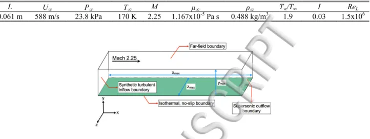
Our simulation is set up similarly to that used in the study of Poggie et al. [19] to enable our results to be easily compared with their data as well as other experimental results produced under similar flow conditions. We consider a supersonic flow over a flat plate at Mach number M=2.25 that is fully turbulent in the region close to the outlet. Based on the freestream properties and the length of the plate (L), the incoming flow has a Reynolds number of 1.5 × 106. Further flow parameters are given in Table I_{, and FIG.} 1 _{shows a schematic of the simulation domain and} boundary conditions.

Table I. Simulation parameters. U¢,P¢, T¢, M, ¢, ¢ are the freestream velocity, pressure, temperature, viscosity and density, respectively. Tw!is the wall temperature, I is the turbulence

intensity at the inlet and ReL is the Reynolds number based on the freestream properties and the

length of the plate (L).

L U¢ P¢ T¢ M ¢ ¢ Tw/Tı" I" ReL

0.061 m 588 m/s 23.8 kPa 170 K 2.25 1.167x10-5 Pa s 0.488 kg/m3 1.9" 0.03 1.5x106

FIG. 1. Schematic representation of the simulation domain, highlighting the boundary conditions used. The dimensions of the domain are xmax/L = 1, ymax/L = 0.05 and zmax/L = 0.05.

Periodic boundary conditions are used in the spanwise (z) direction. In the wall-normal (y) direction, a no-slip isothermal wall (with a temperature TW of 323 K) is used. Supersonic outflow

conditions are imposed at the outlet, while far-field conditions are applied on the upper boundary opposite of the wall. A synthetic turbulent inflow boundary condition is used to produce a freestream flow with a superimposed random turbulence.

The synthetic turbulent inflow boundary condition is based upon the digital filter (DF) method documented in [32,33,34,35,36] and, specifically validated in the framework of the present iLES code CNS3D in [35,36]. According to DF, instead of using a white-noise random perturbation at the inlet, energy modes within the Kolmogorov inertial range scaling with k-5/3, where k is the wavenumber, are introduced into the turbulent boundary layer. No large-scale energy modes scaling with k4 are introduced. A cutoff at the maximum frequency of 50 MHz is applied, since the finest mesh used in this study would under-resolve higher values. The turbulence intensity at

the inlet (I) is set as ±3% of the intensity of the freestream velocity. This perturbation has been found to be sufficient to trigger bypass transition and turbulence downstream (FIG. 2_).

The number of mesh points, mesh spacing, and Mach number are given in Table II_{. We} choose to perform our iLES using relatively fine meshes but still coarser than DNS [19]. This is highlighted in Table II_{, where information about the meshes used in previous DNS studies is} included for comparison and validation. For our mesh spacing (弘検岻, we use the conventional inner variable scaling method 弘検袋 噺 憲邸弘検 荒栂 "where 憲邸 噺 紐酵栂 貢栂 is the friction velocity, 荒栂 the near wall kinematic viscosity, 酵_栂 the near wall shear stress, and 貢_栂 the near wall density.

FIG. 2. Iso-surfaces of Q-criterion colored by Mach number; density gradient magnitude contours plane is in grayscale. For better interpretation of this figure, the reader is referred to the web (colored) version of this article.

Table II. Mesh parameters; nx, ny and nz are the number of mesh points. The “+” sign denotes dimensionless mesh spacing, as defined for 志姿袋"in the text. The subscripts w and e denote wall and boundary layer edge values.

nx ny nz x+ y+w y+e z+ M Present 2591 277 139 9.06 0.497 6.26 8.53 2.25 [19] 4026 276 255 6.0 0.5 9 5.0 2.25 [19] 22548 1277 1131 1.0 0.9 0.9 1.0 2.25 [11,13] 1760 400 800 8.6 0.56 8.9 5.2 2.50 [10,37] 4160 221 440 5.7 0.7 10 4.9 2.00

Our main interest in this study is to determine the accuracy of iLES for performing acoustic loading calculations beneath turbulent supersonic boundary layers. To assess the method, we measure the amplitudes of the pressure fluctuations and analyze their spectral characteristics. We use the Welch method [38] to calculate the power spectral density (PSD) of the pressure fluctuations in specific locations. The sampling frequency is approximately 15.5 MHz, and the overall pressure record is subdivided into 8 segments, each including 2 × 1,200 samples; note that we observe a negligible difference between the PSD produced using 8 and 12 segments.

All of the calculations shown below are performed at the end of the plate in the fully turbulent region, where the boundary layer has the properties presented in Table III_{. Since it is common to} find publications in the literature that report values of Reynolds numbers based on different definitions, we use various formulations, i.e. 迎結_提 噺 貢_著戟_著肯 航_著, 迎結_邸 噺 貢_栂憲_邸絞 航_栂,_! and_! 迎結弟態 噺 貢著戟著肯 航栂, to simplify the comparison of our results with those of past and future publications. The momentum and boundary layer thicknesses are denoted by 肯 and 絞, respectively. The flow statistics at the calculation point are computed by averaging in time over three flow cycles and spatially in the spanwise direction. The statistical convergence of the simulations based on the Standard Error of the Mean (SEM) is less than 2%. The total simulation time for each case is equal to six flow cycles, with the first three omitted from the calculations for statistical purposes. We ensured that statistical convergence in the calculations has been

achieved and that averaging over a longer period would not adversely impact on the accuracy. Furthermore, comparing the present results against theoretical models, DNS and experiments tested the accuracy of iLES.

Table III. Boundary layer properties at the location selected for analysis (姉 鯖 噺 層) of the

acoustic loading for Mach 2.25. The compressible form of momentum (飼) and displacement (諮茅) thicknesses has been used. 殺 噺 諮茅 飼 is the shape factor.

Re Rek Reh2 h (mm) (mm) h* (mm) H

iLES9 2170.0 414.0 1280.6 1.076 0.088 0.314 3.56 iLES5 1806.2 377.1 1065.9 1.012 0.073 0.258 3.51 iLES2 1593.8 344.6 940.5 0.952 0.065 0.241 3.72

III. _RESULTS

A. _{Turbulent Boundary Layer}

We first compare our basic flow statistics (see FIG. 3_{) with DNS results and experimental} data at similar Mach numbers. The purposes of this comparison are to support the reliability of our calculations and to highlight the absence of post-transitional effects. As such, the boundary layer at the calculation point can be considered an accurate approximation of a fully developed supersonic TBL. It is well established that an incompressible TBL has a velocity profile that can be described, at least near a wall, using a one-parameter family of profiles. The most commonly known profile is the logarithmic velocity distribution of von Karman (“law of the wall”):

憲怠 塚帖袋 噺 怠_賃健券岫検袋岻 髪 系,!!!!!!!!!!!!!!!!!!!!!!!!!!!!!!!!!!!!!!!!!!!!!!!!!!!!!!!!!!!!!!!!!!!(1) where 倦 is the von Karman’s constant and 系 is an experimentally derived constant.

In FIG. 3_{a, we give the time-averaged van Driest transformed velocity profiles for all} simulated cases at the end of the plate. The results of the high-order iLES9 perfectly collapse to previous DNS [12,19,37], experimental [39], and incompressible theoretical [40] results. Note that differences in the results in the above studies are also due to the different Reynolds numbers

employed in the simulations and experiments [12]. For example, the past DNS studies have been performed at Re_h2 = 2000 [19] and Reh2 = 1552 [37], while the experiments at Reh2 = 2600 [39].

The present results from the iLES9 simulations correspond to Re_h2 = 1280.6.

Another important statistical quantity calculated and analyzed here is intermittency, which is the probability of the density being less than a threshold value. Poggie et al. [19] defined this threshold as ~97.5% of the freestream density based on the study of the density probability density function (PDF), which was found to be bimodal in the outer part of the boundary layer with a minimum at à 0.975 _ı. The iLES9 results agree very well with the reported experimental hotwire measurements [41,42] and the DNS results of Poggie et al. [19] (see FIG. 3_{b). The small deviation close to the boundary-layer edge can be attributed to the significantly} coarsened mesh we have used in comparison to the DNS study. On the other hand, the results obtained using the low-order iLES (iLES2 and iLES5) fail to follow the reference values, although the simulations are performed using the same mesh as the one used to obtain the iLES9 results. Note that all methods converge in the viscous sublayer and most of the deviations are located in the log-law region. Although the flow statistics obtained using all methods agree perfectly in the viscous sublayer, failure to describe the whole boundary layer correctly may lead to inaccuracies in the calculated pressure signals on the wall.

FIG. 3. Effect of the selected method on boundary layer profiles at 姉 鯖 噺 層. Present results are compared with previous DNS [12,19,37] and experimental data [41], as well as an incompressible theoretical model [40]. The maximum SEM is less than 2%. (a) van Driest transformed streamwise velocity profile as a function of y+. (b) Intermittency profiles of the density through the boundary layer with 誌 噺 皿岷持 隼 宋 操挿捜持_著峅. For better interpretation of these figures, the reader is referred to the web (colored) version of this article that contains the color version of them.

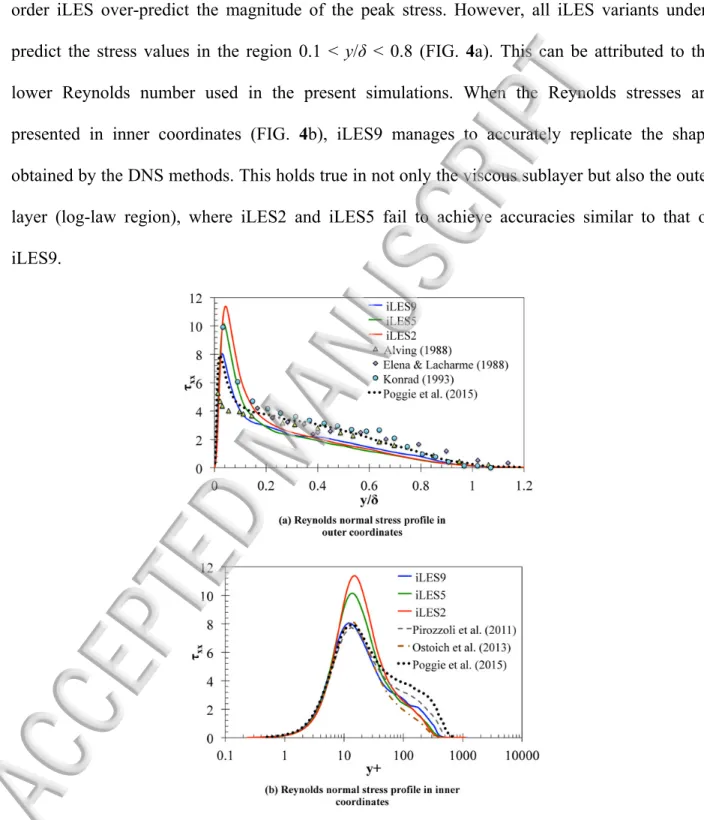
Before presenting and discussing the results of the pressure calculations, we wish to further assess the accuracy of our calculations. It is critical that the boundary layer is described as accurately as possible. From previous DNS studies and experiments, we have access to measurements and calculations of the Reynolds normal stress, 酵_掴掴 噺 貢極憲嫗態玉 岫貢_栂憲_邸態岻, which

accounts for turbulent fluctuations in fluid momentum. Once more, the highest-order iLES successfully predicts the location and magnitude of the peak Reynolds stress, while the lower-order iLES over-predict the magnitude of the peak stress. However, all iLES variants under-predict the stress values in the region 0.1 < y/h < 0.8 (FIG. 4_{a). This can be attributed to the} lower Reynolds number used in the present simulations. When the Reynolds stresses are presented in inner coordinates (FIG. 4_{b), iLES9 manages to accurately replicate the shape} obtained by the DNS methods. This holds true in not only the viscous sublayer but also the outer layer (log-law region), where iLES2 and iLES5 fail to achieve accuracies similar to that of iLES9.

FIG. 4. Effect of selected method on Reynolds normal stress profile, (a) outer coordinates and (b) inner coordinates. Present iLES results are compared with DNS [12,19,37] and experimental data

[39,43,44]. The maximum SEM is less than 2%. For better interpretation of these figures, the reader is referred to the web (colored) version of this article.

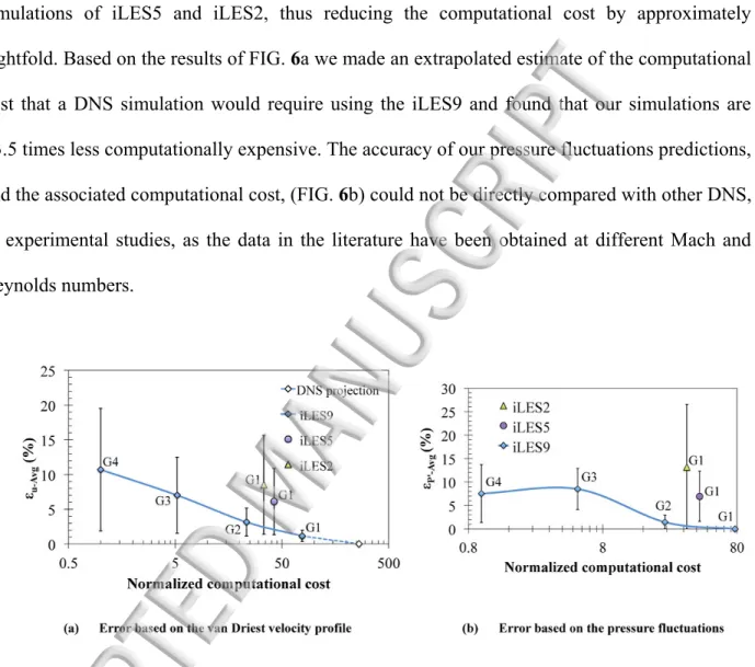
FIG. 5 _{shows the effects of mesh refinement on the velocity profile. The results on mesh G2,} which consists of ~36 million points, differ only by about 2% from those obtained by the finest mesh (G1) consisting of ~100 million points. Using the results from FIG. 3_{a and FIG.} 5 _we calculated the average error of our simulations in comparison to the DNS results of Poggie et al. [19] as:

綱凋塚直 噺 _朝怠デ沈退怠朝 弁通呑灘縄 日_通貸通_{呑灘縄 日}妊認賑濡賑韮禰 日弁"!!!!!!!!!!!!!!!!!!!!!!!!!!!!!!!!!!!!!!!!!!!!!!!!!!!!!!!(2)

where N is the number of points used in the calculation of the average error. The error in the prediction of pressure fluctuations for different iLES variants and different mesh resolutions, and the associated computational cost, are shown in FIG. 6_b.

FIG. 5. Effect of mesh refinement on accuracy, van Driest transformed streamwise velocity profile as a function of y+, all results are from simulations utilizing the highest order iLES. In the legend of the figure the number of mesh points for the streamwise, wall-normal and spanwise direction are given for each case.

The error bars in FIG. 6 _{show the standard deviation of the error from its average value in} various points. Both the mesh size and the iLES order significantly affect the computational cost of the simulation. For each iLES variant the computational cost is normalized by the

computational time of iLES9 on the coarsest mesh (G4). The iLES9 simulations on the coarser mesh G3 (~10.5 million mesh points) can achieve similar accuracy to the finest mesh (G1) simulations of iLES5 and iLES2, thus reducing the computational cost by approximately eightfold. Based on the results of FIG. 6_{a we made an extrapolated estimate of the computational} cost that a DNS simulation would require using the iLES9 and found that our simulations are ~3.5 times less computationally expensive. The accuracy of our pressure fluctuations predictions, and the associated computational cost, (FIG. 6_{b) could not be directly compared with other DNS,} or experimental studies, as the data in the literature have been obtained at different Mach and Reynolds numbers.

FIG. 6. Accuracy and computational cost comparison between the different iLES variants and meshes used. Error bars show the standard deviation of the values from the mean. Mesh labeling is as per legend of Fig. 5. In (a) the comparison is based on the van Driest velocity profile up to y+ = 300. The DNS simulation of Poggie et al. [19] has been used as the reference. In (b) the comparison is based on the pressure fluctuations up to the boundary layer edge. The highest order iLES on the finest mesh G1 has been used as the reference.

Following the same procedure we calculated the average error between the present values of the Reynolds normal stresses and the corresponding DNS [19,37]. Indicatively, the iLES9 approach on the finest mesh averaged a difference of 6.5% from Poggie et al. [19], while

achieving a similar level of accuracy as the DNS results of Pirozzoli et al. [37]. Poggie et al.

[19] obtained these results from a mesh consisting of 3.2 billion points to meet the strict definition requirements of a DNS mesh. The difference of the lower order iLES from the reference DNS was 15% and 24% for iLES5 and iLES2, respectively.

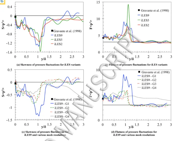
The simulation results were further scrutinized by examining the skewness (鯨極喧嫗玉 噺 極"喧旺戴_{玉 極喧旺}態_玉怠 泰_{) and flatness (繋極喧}嫗_{玉 噺 "極喧旺}替_{玉 極喧旺}態_玉態_{) of the pressure fluctuations. Non-zero values} of skewness and flatness values greater than 3, indicate turbulence anisotropy.

The skewness and flatness of the pressure fluctuations are shown in FIG. 7 _{for the three iLES} variants, as well as for different mesh resolutions. The present wall predictions show good agreement with the experimental measurements of Gravante et al. [45]. At this point skewness has a small negative value, while flatness has a value over 4, indicating that turbulence is non-isotropic, as expected, close to the wall. All iLES variants show very good agreement with the experimental measurements on the wall (FIG. 7_{a,b); however, low resolution meshes (G3 and} G4) fail to correctly predict the high-order statistics on the wall (FIG. 7_c,d).

FIG. 7. Comparison of skewness (a,c) and flatness (b,d) between iLES variants (a,b) and mesh resolutions (c,d). The experimental measurements of Gravante et al. [45] on the wall are presented with black squares. The black lines indicate skewness and flatness values for isotropic turbulence.

All iLES variants have a peak in both skewness and flatness close to the boundary layer edge. This behavior of skewness and flatness near the edge of the boundary layer suggests the dominance of small pressure fluctuations below the mean, whereas large pressure fluctuations are more intense, but less frequent. Away from the edge of the boundary layer, skewness and flatness are close to 0 and 3, respectively, indicating return to isotropy. iLES9 results on the finest mesh gradually tend towards isotropy with respect to both skewness and flatness. iLES5

and iLES2 on the finest mesh predict flatness around 3, similar to iLES9, but for the skewness give a value around -0.2.

Further investigation using finer mesh resolutions is required to understand the connection of the peak in skewness and flatness (Fig. 7) with intermittency effects near the boundary layer edge (as also indicated in Fig. 3b), as well as acoustic radiation effects and their impact on the skewness and flatness values away from the edge of the boundary layer. It has been found that the freestream acoustic pressure fluctuations are non-isotropic and has a preferred wave angle (See Ref. [13]). The above issues would be studied in a future paper by further refining the wall-normal mesh in the free stream in order to resolve the freestream acoustic radiation

B. _{Acoustic loading}

The basic statistical quantity that describes the magnitude of near-wall acoustic loading is the root-mean-square level of the pressure fluctuation (p磯rms). In the experiments, this value is estimated through the integration of power spectral density data, an approach that has to be carefully applied as it can induce errors, which is reflected in the wide spread of the experimental results [8]. More specifically, the experimental results can be contaminated by noise in the low-frequency region of the spectrum owing to background facility noise and vibrations that increase the amplitude of p磯rms. The high-frequency spectrum can also be erroneous owing to sensor spatial resolution limitations, which tend to decrease estimates of the pressure fluctuation intensity.

Historically, p磯rms was non-dimensionalized by the boundary layer edge or freestream dynamic pressure, 圏_著 噺 紘_銚沈追喧_著警_著態 に, with 紘_銚沈追 being the air heat capacity ratio, 喧_著 the freestream pressure and 警_著 the freestream Mach number. We will present our results in this reduced form to compare them directly with previous DNS results and experimental data. We focus on the

near-wall (y/h < 0.2) pressure signals, where our calculations are in very close agreement with the extended value measured and corrected by Beresh et al. [8] and in excellent agreement with the DNS results obtained by Duan and Choudhari [46] (FIG. 8_{a). These results indicate that} previous to Beresh et al. [8] experimental measurements significantly under-predict the acoustic loading on the walls beneath a supersonic TBL. Beresh et al. [8] proposed using the Corcos [47] corrections, which involve combining measurements from multiple sensors while applying noise cancellation (gray filled-in diamond in FIG. 8_{a), as well as an extension to the measured spectra} to minimize the spatial resolution constraints of the sensors (transparent diamond in FIG. 8_a). Both noise cancelation and high-frequency extension seem to drastically improve the quality of the results, although further experiments and simulations are needed to support these findings.

FIG. 8. (a) Pressure fluctuations and (b) compressibility normal to the wall. . Black filled-in diamond is the uncorrected measurement of Beresh et al. [8] at 捌 噺 匝 捜; grey filled-in diamond is the noise corrected measurement; and transparent diamond corresponds to the extended value. Light blue circle is the theoretical prediction of Laganelli et al. [48] and the dashed line is from the DNS results of Duan and Choudhari [46] at 捌 噺 匝 捜. The maximum SEM is less than 2%. For better interpretation of these figures, the reader is referred to the web (colored) version of this article.

In the near-wall region that is critical to our acoustic loading study, the results of the two higher-order iLES show a very good agreement with each other, while the lower-order iLES over-predicts the intensity of the pressure fluctuations (FIG. 8_{a). Further away from the wall, but} still inside the boundary layer, iLES5 produces results closer to the DNS results than iLES9 does. This finding can be a result of the dispersive nature of the highest-order variant, but further examination is necessary before drawing a definitive conclusion.

The operative cause for developing a reduced form for pressure fluctuations and other results was an attempt made in previous years to link compressible flows to incompressible ones, for which theoretical and experimental data are more accessible. This effort led to the development of theoretical models that attempted to predict — or scale — the pressure fluctuation intensity based on measurements of incompressible flows. A characteristic example of such a theoretical model is the relation proposed by Laganelli et al. [48]:

使司仕史嫦

刺屯 噺

宋 宋宋掃

岷宋 捜袋岫参始 参珊始岻盤宋 捜袋宋 宋操捌屯匝 匪袋宋 宋想捌屯匝峅宋 掃想. (3)

In the above equation, Taw is the adiabatic wall temperature calculated from the definition of

the recovery temperature. The formula is linked to the incompressible database through the value 0.006, which is believed to be biased low due to the insufficient sensor spatial resolution in the era in which most experiments were carried out. Later publications suggest that this value should be corrected to 0.009 [8,49]. In FIG. 8_{a, we show the prediction based on the original model}

proposed by Laganelli et al. [48]. Applying the suggested correction (0.009) raises the value close to the point predicted by the extended measurement of Beresh et al. [8].

The example above suggests that empirical models based on incompressible, or even compressible, data must be used with caution as they are influenced by the conditions inherent to each experimental facility. In addition, since density gradients in the boundary layer — especially close to the wall — are very high (FIG. 8_{b), we expect compressibility effects to play} a significant role in acoustic loading. Further away from the wall, the density converges to the freestream value very quickly, while outside the boundary layer, the density fluctuations diminish.

Considering that our calculations on the wall are of comparable accuracy to DNS results and the latest experimental measurements, we can further analyze the pressure signals. In acoustic loading calculations, it is common to transform the fluctuating pressures to sound pressure level (SPL), which can be directly connected to high cycle fatigue in aerospace structures:

鯨鶏詣 噺 にど"健剣訣怠待岾椎認尿濡 嫦

態待禎牒銚峇. (4)

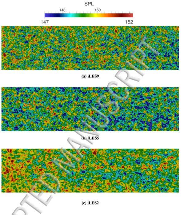
Using all three iLES variants, we calculate the SPL on the plate beneath the TBL. Instead of presenting the SPL values for specific locations, we take advantage of the nature of computer simulations and compile SPL contour plots over the entire plate (FIG. 9_{). Although the range of} values achieved by all iLES is similar, a higher-order variant produce much finer- and smaller-scaled structures than a lower-order iLES. This unsteady nature of acoustic loading can increase the propensity for high cycle fatigue of the material on the vehicle outer mold-line.

FIG. 9. Snapshot of the SPL calculation on the plate in the fully turbulent region with three different orders of accuracy, a) iLES9, b) iLES5, and c) iLES2. For better interpretation of these figures, the reader is referred to the web (colored) version of this article.

As mentioned at the beginning of this section, most experimental information comes from measurements of the frequency spectrum of the wall pressure fluctuations. This quantity provides information about the distribution of the pressure fluctuations energy in frequency

space, and there have been considerable efforts to characterize its shape and identify its scaling laws. The frequency spectrum of the pressure field is defined as

肢岫磁岻 噺_匝慈層 完 使著 博博博博博博博博博博博博博博博博博博博博博博博博博博博博博博博博博博博蚕嫗_{岫姉 姿 子 嗣岻使}嫗_{岫姉 姿 子 嗣 髪 滋岻} 貸餐磁滋_纂滋

貸著 , (5) where 酵 is a time delay and 降 is radial frequency.

The results we present are again from the same calculation points at which all previous statistics have been calculated. In the low-frequency region, the two high-order iLES show almost perfect agreement, while the low-order iLES2 peaks at a much higher value (FIG. 10_{). In} contrast to the high-frequency region, where viscosity and near-wall motions are the key parameters, the low-frequency region is mostly affected by large-scale velocity fluctuations. In the higher-frequency region, low-order iLES lose energy much more rapidly than the highest-order iLES9, with the latter being more accurate, as the following comparison with the DNS and experimental data will reveal.

FIG. 10. Normalized power density spectrum of computed pressure signal on the wall at location

x/L =1. Comparison with DNS [10,11,13] and experimental data [8] of compressible flows at

M=2 and M=2.5. Black dashed straight lines are guides for the eye. For better interpretation of this figure, the reader is referred to the web (colored) version of this article.

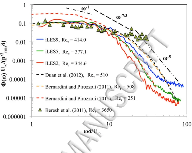
In FIG. 10_{, we also compare our results to the DNS data of Bernardini and Pirozzoli [10] and} Duan et al. [11,13], who used slightly different Mach numbers, M = 2 and 2.5, respectively. Another difference between the simulations is the properties of the boundary layer, and more specifically, the friction Reynolds number (Re_k) that can affect the amplitude of the pressure fluctuations, especially in the high-frequency region. Considering that the friction Reynolds numbers obtained by Bernardini and Pirozzoli [10] are either smaller or greater than those obtained from the present simulations, we expect our PSD to lie somewhere in between the two.

Only the results of the highest-order iLES satisfy this estimate, with the lower-order iLES significantly deviating from it.

To further assess the quality of our calculations, we compare our results with experimental data [8] and theoretical scaling predictions. Owing to the sensor spatial resolution limitations mentioned previously, the available experimental data include measurements only in the low-frequency region. Since the friction Reynolds number does not significantly affect this low-frequency region, a comparison can still be made, even though the experimental boundary layer is significantly thicker. Our results, as well as those in the reference cases, decay very weakly as

降

In the mid-frequency range, a universal overlap region is expected with -1 scaling following the prediction of Bradshaw [54] and later theoretical [55] and experimental verifications [8,45]. The highest order iLES reproduces this slope only for a short frequency range between 300 kHz and 500 kHz (see FIG. 11_{a). The} -1 _{scaling is induced by eddies in the logarithmic region of the} boundary layer. This scaling region appears only at sufficiently high Reynolds numbers, while the slope decreases, or diminishes, for lower Reynolds numbers; this explains the occurrence of

-1

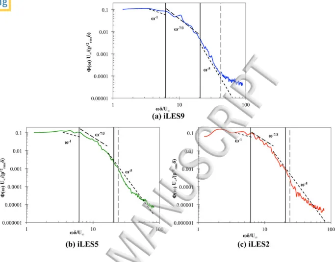
FIG. 11. Normalized power density spectrum of computed pressure signal on the wall at location 姉 鯖 噺 層. Comparison between theoretical scaling predictions and the calculated results from a) iLES9, b) iLES5 and c) iLES2. Black vertical lines indicate the transition between different frequency regions according to the theory. Grey vertical dashed line show the maximum resolved frequency for each iLES. Black dashed lines indicate the gradient of the various frequency regions.

At higher frequencies, the spectrum should roll off at a higher rate, reaching a slope proportional to -5, predicted theoretically by Blake [56] and measured in previous experiments [45,57]. Thus, the spectrum should transition from the mid- to the high-frequency region, where small-wavelength eddies become dominant much closer to the wall [45]. This transition region has been observed in experiments on incompressible flows [57,58], with its onset found to be near /uk2 = 0.3 [57]. In the present iLES9 simulations, this value is equivalent to about f = 536

kHz (first vertical black line in FIG. 11_{). The spectrum at this transitional region is believed to be} proportional to -7/3 [59], fully reaching -5 dependency at around /u_k2 = 1 (or f = 1.8 MHz for iLES9, second vertical black line in FIG. 11_{) [58]. The black dashed lines in Figs. 8 and 9} indicate the gradient while the vertical solid lines show the transition from one frequency region to the other according to this analysis. Only the high-order iLES9 manages to capture all three regions with the correct spectrum roll off slopes from low- to high-frequency ranges. It is also the only method that correctly resolves all frequencies up to 3.9 MHz (grey dashed line in FIG. 11_{c), while the lower order methods produce a steeper slope than} -5 _{for frequencies greater than} 2.2MHz (grey dashed line in FIG. 11_{a and b).}

Note that in relation to the effects of acoustic loading on structural fatigue special attention is given to the initial region (spectrum proportional to 0) where the low-frequency content will affect the structural response and fatigue life of panel structures. In the aforementioned figures we showed the complete pressure spectrum roll-off in logarithmic plots, while in FIG. 12 _we show the same spectrum limited to the low frequency region in a linear plot. The highest order iLES produces results that follow closely the previously published DNS calculations with an average difference of ~ 5% from them. In contrast, the low order iLES2 over-predicts the pressure spectrum in this region, threefold with reference to DNS, and the results also exhibit an (non-physical) oscillatory behavior. The differences between the iLES variants observed in this low frequency region, as well as in the whole pressure spectrum roll-off, are also correlated with the pressure fluctuations on the wall (see FIG. 8_a).

FIG. 12. Normalized power density spectrum of the low frequency region. Comparison with previous DNS results (dashed lines) [10,11,13]. For better interpretation of this figure, the reader is referred to the web (colored) version of this article.

A correlation can be drawn between the resolved turbulent length scales and the calculated spectrum of the pressure fluctuations on the wall. A previous study [18] has shown how the order of the method affects the shape and magnitude of the energy spectra, with the iLES9 approach providing results that closely match those of DNS. In the previous paragraphs we elaborated upon the better agreement of iLES9 with DNS, experimental and theoretical values of PSD. One can conclude that any method capable of resolving finer structures (see FIG. 2 _{and FIG.} 9_{) also} provides a more accurate energy and pressure spectrum. Failing to correctly reproduce small scales seems to directly affect the energy distribution across all scales.

In addition to the last figure we conduct an analysis of the distribution of energy along the entire frequency spectrum. The pre-multiplied pressure spectra on the wall, along with the calculations of Duan et al. [11,13], are plotted in FIG. 13_{. The highest-order iLES produces a} peak at around h/U_ı = 8 (or f = 696 kHz), similar to the results reported by Duan et al. [11,13] but with the higher amplitude characteristic of a higher friction Reynolds number. The two lower-order iLES fail to correctly capture the position of the maxima and cause a shift in the

pre-multiplied pressure spectrum toward the lower-frequency band. This pressure spectrum shift can also be correlated with the SPL structures in FIG. 9 _{where iLES2 resolves large and coarse} structures that contain low frequency pressure fluctuations energy, contrary to the smaller and finer (high frequency pressure fluctuations) structures of the higher order iLES (see FIG. 13). From a structural point of view fatigue estimation on aerospace structures depends not only on the amplitude of acoustic loading but also on the frequency range in which the highest amplitude is observed.

FIG. 13. Pre-multiplied power density spectrum of pressure signals on the wall at location 姉 鯖 噺 層. Direct comparison with DNS results [11,13]. For better interpretation of this figure, the reader is referred to the web (colored) version of this article.

The present iLES approach produces high-fidelity results that closely match previous DNS studies but require only a fraction of the computational cost. The promising conclusion about the iLES approach is further supported by the findings of Poggie et al. [19] where good agreement between iLES and DNS was also shown, with iLES requiring significantly less computational resources than DNS.

Our simulations utilized 480–720 cores on the Archie-WeSt supercomputer, which consists of 3500 Intel Xeon X5650 cores and 4GB of RAM per core, whereas the most recent DNS results required 23,040–102,400 cores [19].

IV. _CONCLUSIONS

In the previous sections, we compared our calculations of acoustic loading beneath a supersonic attached TBL with previous numerical and experimental data as well as with the results predicted by various theoretical models where possible. We concluded that the iLES approach can achieve high levels of accuracy in the near wall region that are directly comparable to the results produced by DNS but require only a fraction of the computational resources.

In addition, we demonstrated that iLES provides good acoustic loading estimations, which are in agreement with DNS data and the most recently filtered and corrected experimental measurements. In addition to the magnitude of acoustic loading in space, we analyzed our data in the frequency domain. The pressure spectrum roll off was found to be heavily affected by the state of the boundary layer and the freestream conditions, i.e., compressibility effects in the low-frequency region dictate the slope of the pressure amplitude as the low-frequency, or the Reynolds number, approaches zero.

In presenting our results, we also discussed the differences between high- and low-order iLES and how the latter can introduce significant errors. We observed, for example, that the energy of the high-frequency pressure spectrum is underestimated by low-order iLES, while in the

mid-range frequency region the position of the maxima is also inaccurate. This can be attributed to the numerical dissipation of low-order iLES methods, which can artificially damp turbulent eddies and their associated sound spectra, particularly in the high- and mid-frequency ranges.

The results of this study reduce the uncertainties in acoustic loading simulations on structures beneath TBL while highlighting the capabilities of iLES in this field. Further simulations at higher Reynolds and Mach numbers will allow us to further assess iLES by comparing our results with experimental and flight data.

ACKNOWLEDGMENTS

This work was sponsored by the Air Force Office of Scientific Research, Air Force Material Command, USAF, under grant number FA9550-14-1-0224. The U.S. Government is authorized to reproduce and distribute reprints for Governmental purpose notwithstanding any copyright notation thereon. Results were obtained using the EPSRC funded ARCHIE-WeSt High Performance Computer (www.archie-west.ac.uk) under EPSRC grant no. EP/K000586/1.

[1] J.W. Miles, "On structural fatigue under random loading," Journal of Acoustical Society of America, vol. 21, no. 11, pp. 753-762, 1954.

[2] A. Powell, "On the fatigue failure of structures due to pressure fields," Journal of Acoustical Society of America, vol. 30, no. 12, pp. 1130-1135, 1958.

[3] B. L. Clarkson, "Stresses in skin panels subjected to random acoustic loads," The Aeronautical Journal, vol. 72, no. 695, pp. 1000-1010, 1968.

[4] B. L. Clarkson, "Review of sonic fatigue technology," NASA, Technical Report CR-4587, 1994.

[5] P. R. Cunningham and R.G White, "A review of analytical methods for aircraft structures subjected to high-intensity random acoustic loads," Proceedings of the Institution of Mechanical Engineers, Part G: Journal of Aerospace Engineering, vol. 218, no. 3, pp. 231-242, 2004.

[6] B. A. Miller, J. McNamara, S. M. Spottswood, and A. Culler, "The impact of flow induced loads on snap-through behavior of acoustically excited, thermally buckled panels," Journal of Sound and Vibration, vol. 330, no. 23, pp. 5736-5752, 2011.

[7] M. P. Mignolet, A. Przekop, S. A. Rizzi, and S. M. Spottswood, "A review of indirect/non-intrusive reduced order modeling of nonlinear geometric structures," Journal of Sound and Vibration, vol. 332, no. 10, pp. 2437-2460, 2013.

[8] S. J. Beresh, J. F. Henfling, R. W. Spillers, and B. O. M. Pruett, "Fluctuating wall pressures measured beneath a supersonic turbulent boundary layer," Physics of Fluids, vol. 23, no. 7, 2011.

[9] J. D. Schmisseur, "Hypersonics into the 21st century: A perspective on AFOSR-sponsered research in aerothermodynamics," Progress in Aerospace Sciences, vol. 72, pp. 3-16, 2015.

Physics of Fluids, vol. 23, no. 8, 2011.

[11] L. Duan, M. M. Choudhari, and M. Wu, "Numerical Study of Pressure Fluctuations due to High-Speed Turbulent Boundary Layers," 42nd AIAA Fluid Dynamics Conference and Exhibit, Paper No. NF1676L-13740, (New Orleans, June 1-16, 2012), pp. 1-16.

[12] C.M. Ostoich, D.J. Bodony, and P.H. Geubelle, "Interaction of a Mach 2.25 turbulent boundary layer with a fluttering panel using direct numerical simulation," Physics of Fluids, vol. 25, no. 11, 2013.

[13] L. Duan, M. M. Choudhari, and M. Wu, "Numerical study of acoustic radiation due to a supersonic turbulent boundary layer," Journal of Fluid Mechanics, vol. 746, pp. 165-192, 2014.

[14] L. Duan, M. M. Choudhari, and C. Zhang, "Pressure fluctuations induced by a hypersonic turbulent boundary layer," Journal of Fluid Mechanics, vol. 804, pp. 578-607, 2016.

[15] J. Boris, F. Grinstein, E. Oran, and R. Kolbe, "New insights into large eddy simulation," Fluid Dynamics Research, vol. 10, no. 4-6, pp. 199-228, 1992.

[16] C. Fureby and F. F. Grinstein, "Large Eddy Simulation of High-Reynolds-Number Free and Wall-Bounded Flows," Journal of Computational Physics, vol. 181, no. 1, pp. 68-97, 2002.

[17] L. G. Margolin, W. J. Rider, and F. F. Grinstein, "Modeling turbulent flow with implicit LES," Journal of Turbulence, vol. 7, no. 15, 2006.

[18] I. W. Kokkinakis and D. Drikakis, "Implicit Large Eddy Simulation of weakly-compressible turbulent channel flow," Computer Methods in Applied Mechanics and Engineering, vol. 287, pp. 229-261, 2015.

[19] J. Poggie, N. J. Bisek, and R. Gosse, "Resolution effects in compressible, turbulent boundary layer simulations," Computers and Fluids, vol. 120, pp. 57-69, 2015.

[20] D. J. Bodony and S. K. Lele, "On using large-eddy simulation for the prediction of noise from cold and heated turbulent jets," Physics of Fluids, vol. 17, 2005.

[21] D. J. Bodony and S. K. Lele, "Current Status of Jet Noise Predictions Using Large-Eddy Simulation," AIAA Journal, vol. 46, no. 2, pp. 364-380, 2008.

[22] S. Unnikrishnan, L. Agostini, and D. V. Gaitonde, "Analysis of Intermittency of Supersonic Jet Noise with Synchronized LES," 21st AIAA/CEAS Aeroacoustics Conference, Paper No. AIAA 2015-2532, (Dallas, June 2015).

[23] B. Thornber, D. Drikakis, D. L. Youngs, and R. J. R. Williams, "The Influence of Initial Conditions on Turbulent Mixing due to Richtmyer-Meshkov Instability," Journal of Fluid Mechanics, vol. 654, pp. 99-139, 2010.

[24] M. Hahn, D. Drikakis, D. L. Youngs, and R. J. R. Williams, "Richtmyer–Meshkov turbulent mixing arising from an inclined material interface with realistic surface perturbations and reshocked flow," Physics of Fluids, vol. 23, 2011.

[25] E. F. Toro, M. Spruce, and W. Speares, "Restoration of the contact surface in the HLL-Riemann solver," Shock Waves, vol. 4, no. 1, pp. 25-34, 1994.

[26] E. F. Toro, Riemann Solvers and Numerical Methods for Fluid Dynamics, 3rd ed.: Springer, 2009.

[27] B. van Leer, "Towards the ultimate conservative difference scheme III. Upstream-centered finite-difference schemes for ideal compressible flow," Journal of Computational Physics, vol. 23, no. 3, pp. 263-275, 1977. [28] K. H. Kim and C. Kim, "Accurate, efficient and monotonic numerical methods for multidimensional

compressible flows: Part II: Multidimensional limiting process," Journal of Computational Physics, vol. 208, no. 2, pp. 570-615, 2005.

[29] D. S. Balsara and C.-W. Shu, "Monotonicity preserving weighted essentially non-oscillatory schemes with increasingly high order of accuracy," Journal of Computational Physics, vol. 160, no. 2, pp. 405-452, 2000. [30] R.J. Spiteri and S. J. Ruuth, "New Class of Optimal High-Order Strong-Stability-Preserving Time

Discretization Methods," SIAM Journal on Numerical Analysis, vol. 40, no. 2, pp. 469-491, 2002. [31] P. Tsoutsanis et al., "Comparison of structured and unstructured-grid, compressible and incompressible

methods using the vortex pairing problem," Computer Methods in Applied Mechanics and Enginnering, vol. 293, pp. 207-231, 2015.

[32] T. S. Lund, X. Wu, and K. D. Squires, "Generation of turbulent inflow data for spatially-developing boundary layer simulations," Journal of Computational Physics, vol. 140, no. CP975882, pp. 233-258, 1998.

[33] M. Klein, A. Sadiki, and J. Janicka, "A digital filter based generation of inflow data for spatially developing direct numerical or large eddy simulations," Journal of Computational Physics, vol. 186, pp. 652-665, 2003. [34] E. Touber and N. D. Sandham, "Large-eddy simulation of low-frequency unsteadiness in a turbulent

shock-induced separation bubble," Theoretical and Computational Fluid Dynamics, vol. 23, pp. 79-107, 2009. [35] Z. A. Rana, B. Thornber, and D. Drikakis, "On the importance of generating accurate turbulent boundary

condition for unsteady simulations," Journal of Turbulence, vol. 12, no. 35, pp. 1-39, 2011.

[36] Z. A. Rana, B. Thornber, and D. Drikakis, "Transverse jet injection into a supersonic turbulent cross-flow,"

Physics of Fluids, vol. 23, no. 046103, pp. 1-21, 2011.

[37] S. Pirozzoli and M. Bernardini, "Turbulence in supersonic boundary layers at moderate Reynolds number,"

Journal of Fluid Mechanics, vol. 688, pp. 120-168, 2011.

[38] P. D. Welch, "The use of Fast Fourier Transform for the Estimation of Power Spectra: A Method Based on Time Averaging Over Short, Modified Periodograms ," IEEE Trans. Audio Electroacoustics, vol. AU-15, pp. 70-73, 1967.

[39] M. Eléna and J. P. Lacharme, "Experimental study of a supersonic turbulent boundary layer using a laser Doppler anemometer," Journal de Méchanique Théorique et Appliquée, vol. 7, no. 2, pp. 90-175, 1988. [40] J. M. Österlund, A. V. Johansson, H. M. Nagib, and M. H. Hites, "A note on the overlap region in turbulent

boundary layers," Physics of Fluids, vol. 12, no. 1, pp. 1-4, 2000.

[41] S. Corrsin and A. K. Kistler, "Free-Stream Boundaries of Turbulent Flows," National Advisory Committee for Aeronautics, Technical Report NACA-TR-1244, 1955.

[42] J. Andreopoulos, K. C. Muck, J. P. Dussauge, A. J. Smits, and M. S. Selig, "Turbulence structure in a shock wave/turbulent boundary-layer interaction," AIAA Journal, vol. 27, no. 7, pp. 9-862, 1989.

[43] A. E. Alving, "Boundary layer relaxation from convex curvature ," Princeton University, PhD dissertation 1988.

[44] W. Konrad, "A three-dimensional supersonic turbulent boudanry layer generated by an isentropic compression ," Princeton University, PhD dissertation 1993.

[45] S. P. Gravante, A. M. Naguip, C. E. Wark, and H. M. Nagip, "Characterization of the pressure fluctuations under a fully developed turbulent boundary layer," AIAA Journal, vol. 36, no. 10, pp. 1808-1816, 1998. [46] L. Duan and M. M. Choudhari, "Numerical study of pressure fluctuations due to a Mach 6 turbulent boundary

layer," 51st AIAA Aerospace Sciences Meeting, Paper No. AIAA 2013-0532, (Grapevine, Texas, January 7-10, 2013).

[47] G.M. Corcos, "Resolution of pressure in turbulence," Journal of Acoustical Society of America, vol. 35, no. 2, pp. 192-199, 1963.

[48] A. L. Laganelli, A. Martellucci, and L. L. Shaw, "Wall Pressure Fluctuations in Attached Boundary-Layer Flow," AIAA Journal, vol. 21, no. 4, pp. 495-502, April 1983.

[49] M. K. Bull, "Wall-Pressure Fluctuations Beneath Turbulent Boundary Layers: Some Reflections on Forty Years of Research," Journal of Sound and Vibration, vol. 190, no. 3, pp. 299-315, 1996.

[50] J. E. Ffowcs Williams, "Surface pressure fluctuations induced by boundary layer flow at finite Mach number,"

Journal of Fluid Mechanics, vol. 22, no. 507, pp. 507-519, 1965.

[51] R. H. Kraichnan, "Pressure Fluctuations in Turbulent Flow over a Flat Plate," Acoustical Society of America, vol. 28, no. 3, pp. 378-391, 1956.

[52] O. M. Phillips, "On the aerodynamic surface sound from a plane turbulent boundary layer," Proceedings of the Royal Society A, vol. 234, no. 1198, pp. 327-335, 1956.

[53] A. P. Dowling, "Underwater Flow Noise," Theoretical and Computational Fluid Dynamics , vol. 10, pp. 135-153, 1998.

[54] P. Bradshaw, "Inactive motion and pressure fluctuations in turbulent boundary layers," Journal of Fluid Mechanics, vol. 30, no. 2, pp. 241-258, 1967.

[55] R. L. Panton and J. H. Linebarger, "Wall pressure spectra calculations for equilibrium boundary layers,"

Journal of Fluid Mechanics, vol. 65, no. 2, pp. 261-287, 1974.

[57] T. M. Farabee and M. J. Casarella, "Spectral features of wall pressure fluctuations beneath turbulent boundary layers," Physics of Fluids A, vol. 3, no. 10, 1991.

[58] M. C. Goody and R. L. Simpson, "Surface pressure fluctuations beneath two- and three-dimensional turbulent boundary layers," AIAA Journal, vol. 38, no. 10, pp. 1822-1831, 2000.