econ
stor
www.econstor.eu
Der Open-Access-Publikationsserver der ZBW – Leibniz-Informationszentrum WirtschaftThe Open Access Publication Server of the ZBW – Leibniz Information Centre for Economics
Nutzungsbedingungen:
Die ZBW räumt Ihnen als Nutzerin/Nutzer das unentgeltliche, räumlich unbeschränkte und zeitlich auf die Dauer des Schutzrechts beschränkte einfache Recht ein, das ausgewählte Werk im Rahmen der unter
→ http://www.econstor.eu/dspace/Nutzungsbedingungen nachzulesenden vollständigen Nutzungsbedingungen zu vervielfältigen, mit denen die Nutzerin/der Nutzer sich durch die erste Nutzung einverstanden erklärt.
Terms of use:
The ZBW grants you, the user, the non-exclusive right to use the selected work free of charge, territorially unrestricted and within the time limit of the term of the property rights according to the terms specified at
→ http://www.econstor.eu/dspace/Nutzungsbedingungen By the first use of the selected work the user agrees and declares to comply with these terms of use.
zbw
Leibniz-Informationszentrum Wirtschaft Schmidt, Robert; Leitner, JohannesWorking Paper
A systematic comparison of professional exchange
rate forecasts with judgmental forecasts of novices :
Are there substantial differences?
Würzburg economic papers, No. 49 Provided in cooperation with:
Julius-Maximilians-Universität Würzburg
Suggested citation: Schmidt, Robert; Leitner, Johannes (2004) : A systematic comparison of professional exchange rate forecasts with judgmental forecasts of novices : Are there
No. 49
A systematic comparison of professional exchange rate
forecasts with judgmental forecasts of novices
–
Are there substantial differences?
Johannes Leitner and Robert Schmidt
March 2004
Universität Würzburg
Lehrstuhl für Volkswirtschaftslehre, Geld
und internationale Wirtschaftsbeziehungen
Sanderring 2, D-97070 Würzburg
[email protected]W. E. P.
Postal address:
Dr. Johannes Leitner,
Institut für Statistik und Operations Research Universität Graz Universitätsstraße 15/E3 8010 Graz (Austria) Tel: +43-316-380-7245 Fax: +43-316-380-9560 Email: [email protected] Robert Schmidt
Lehrstuhl für Volkswirtschaftslehre, Geld und internationale Wirtschaftsbeziehungen Universität Würzburg Sanderring 2 D- 97070 Würzburg Tel: +49-931-31-2945 Fax: +49-931-31-2775 Email: [email protected] Homepage: http://www.kfunigraz.ac.at/soowww/index.html http://www.wifak.uni-wuerzburg.de/vwl1.htm
A systematic comparison of professional exchange rate forecasts with
judgmental forecasts of novices – Are there substantial differences?
#February 2004
Johannes Leitner, University of Graz Robert Schmidt, University of Wuerzburg
Abstract
The study at hand deals with the expectations of professional analysts and novices in the context of foreign exchange markets. We analyze the respective forecasting accuracy and our results indicate that there exist substantial differences between professional forecasts and judgmental forecasts of novices. In search of reasonable explanations for the astonishing result, we evaluate the nature of professional and experimental expectations in more detail and find that while professional exchange rate forecasts seem to be biased predictors for the future exchange rates, judgmental forecasts appear to be unbiased. Furthermore, professional forecasters consistently expect a reversal of forgoing exchange rate changes whereas novices expect a continuation of current movements in the short-run and are reversed in the long-run.
JEL-classification: C 53, C 92, D 7, D 81, D84, E 27, F 31, F 47, G 12, G 15. Keywords: Foreign exchange market, forecasting, behavioral finance, anchoring
heuristics, judgment, expertise, expectation formation.
# The authors would like to thank Prof. Dr. Peter Bofinger and Prof. Dr. Martin Kukuk for their helpful
Content
1 Introduction ... 1
2 Analysis of professional exchange rate forecasts... 2
2.1 Data... 2
2.2 Accuracy of professional exchange rate forecasts... 3
3 Experimental analysis of human forecasting behavior... 6
3.1 Experiment design ... 6
3.2 Accuracy of experimental forecasts ... 8
4 The nature of expectations... 10
4.1 Rational expectation hypothesis ... 10
4.1.1 Rationality of professional exchange rate forecasts ... 11
4.1.2 Rationality of experimental forecasts... 15
4.2 Different expectation formation mechanisms?... 19
4.2.1 Adaptive expectations ... 19
4.2.1.1 Adaptive expectations of professional forecasts ... 19
4.2.1.2 Adaptive expectations of judgmental forecasts... 20
4.2.2 Extrapolative expectations... 20
4.2.2.1 Extrapolative expectations of professional exchange rate forecasts .. 21
4.2.2.2 Extrapolative expectations of judgmental forecasts ... 23
4.3 Discussion of the results... 24
5 Conclusion... 28
Figures
Figure 1: Available exchange rate forecasts... 3Figure 2: Screenshot of the computer experiment... 7
Figure 3: Experimental time series and forecasts... 8
Figure 4: Expectation errors of survey data... 11
Figure 5: Scatter diagrams for the unbiasedness hypothesis of professional exchange rate forecasts... 13
Figure 6: Expectation errors for experimental forecasts ... 16
Figure 7: Scatter diagrams for the unbiasedness hypothesis ... 16
Figure 8: Expected versus previous exchange rate changes... 22
Figure 9: Expected versus previous change in the experimental time series ... 23
Figure 10: Professional exchange rate forecasts and fundamental exchange rates ... 26
Tables
Table 1: Available forecast data ... 2
Table 2: Accuracy of professional forecasts... 4
Table 3: Tests of differences in professional forecast errors... 4
Table 4: 2x2 contingency table of the χ2-test ... 5
Table 5: Professional forecasts as direction of change forecasts... 6
Table 6: Accuracy of experimental forecasts ... 9
Table 7: Tests of differences in experimental forecast errors ... 9
Table 8: Experimental forecasts as direction of change forecasts... 9
Table 9: Test of unbiasedness for the US-$/€ market forecasts ... 12
Table 10: Test for serial correlation in professional forecast errors... 14
Table 11: Orthogonality test for professional exchange rate forecasts ... 15
Table 12: Test of unbiasedness for the judgmental forecasts... 17
Table 13: Test for serial correlation in experimental forecast errors ... 17
Table 14: Orthogonality test for the judgmental forecasts ... 18
Table 15: Test for adaptive expectations of professional forecasts... 20
Table 16: Test for adaptive expectations of judgmental forecasts ... 20
Table 17: Test for extrapolative expectations of professional forecasts ... 21
Table 18: Test for extrapolative expectations of judgmental forecasts ... 24
Table 19: Selected estimates for the US-$/€ fundamental equilibrium rate... 25
1 Introduction
The empirical failure of standard economic exchange rate models has been proven at least since the seminal work of Meese and Rogoff, [1983a, 1983b]. Rogoff, [2001] subsumes the current status very accurately when he states: “To make a long story short not only have a subsequent twenty years of data and research failed to overturn the Meese-Rogoff result, they have cemented it …”. According to the standard macroeconomic exchange rate models expectations play a decisive role in the determination of exchange rates. It is usually assumed that expectations are formed rationally, i.e. market participants process all available information on the basis of the “correct” exchange rate model. Thereby the considered information set typically consists of macroeconomic fundamentals like money supplies, interest rates, inflation rates.
The aim of this study is to analyze the human expectation formation in more detail. Basically, two different approaches can be identified in the literature regarding the analysis of expectation formation. On the one hand, expectation formation is analyzed within empirical studies. These studies use survey expectations collected by suppliers of financial data. On the other hand, experimental studies draw on expectations collected from subjects in a laboratory. This study considers both ways of analyzing human expectation formation and contrasts both results against each other.
In a large number of mostly experimental studies the influence of expertise on the forecasting performance was analyzed. The comparison of experts and novices has repeatedly revealed that novices’ forecasts are more accurate, a finding which was called the inverted expertise effect. Steal von Holstein and C.A., [1972] compared stock price predictions of statisticians, students, university teachers, market experts and bankers. While the performance of all subjects was poor, contrary to expectations, the one of the bankers was the worst. In a replication of the experiments by Yates et al., [1991], Önkal-Atay and Muradoglu, [1996] supported their finding that students with prior investment experience (i.e. semi-experts) performed worse than unexperienced students in a stock price forecasting task. While these two studies were limited to students, Önkal-Atay and Muradoglu, [1996] asked portfolio managers (experts), bank managers (semi-experts) and business students (novices) for probability forecasts of under different task formats. They could not find general support for the inverted expertise effect.
In our present study we compare point forecasts of the €/US-$ exchange rate surveyed from professional analysts and experimentally generated point forecasts of students for a simulated exchange rate time series. Our analysis is focused on the aggregated level of consensus forecasts, thus we compare average behavior and neglect the behavior of individuals. There are many studies about accuracy especially, in the context of earnings forecasts of financial analysts (for a concise review we refer to Brown, [1993]). However, in the context of foreign exchange rates studies dealing with the forecasting accuracy are rather rare. The focus of studies related to exchange rate expectations rather deal with the question whether expectations are rational (see e.g. Cavaglia et al., [1994])
Overall, we investigate forecasts for three different forecasting horizons: one-step, three-step and six-step ahead forecasts. With our systematic analysis of professional exchange rate forecasts and judgmental forecasts of novices, we try to find differences and similarities in the human expectation formation that allow us to derive possible explanations for the poor forecasting accuracy of the professional exchange rate forecasters.
The reminder of the study is as follows. In the next section we explore the forecasting accuracy of professional exchange rate forecasters. Afterwards, the forecasting accuracy of students’ experimental forecasts are examined. In section 4, we analyze the nature of expectations in more detail. In particular, we investigate the rationality of professional and experimental forecasts. Furthermore, we evaluate whether professional and experimental forecasts are adaptive and extrapolative. Finally, we discuss our results and provide a possible explanation for the poor forecasting performance of professional exchange rate forecasts compared to the experimental forecasts of novices.
2 Analysis of professional exchange rate forecasts
2.1 Data
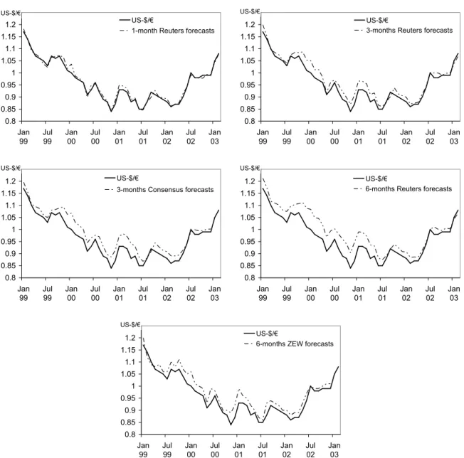
Our analysis of professional forecasts is based on survey data provided by three different suppliers of financial data: Reuters, Consensus Economics and ZEW Finanzmarkttest from the Centre for European Economic Research (ZEW).1 The period under consideration starts in January of 1999 and ends in March of 2003. The available forecast horizons vary depending on the supplier and are summarized in Table 1. Figure 1 shows the survey data that was received at a given date for different time horizons. The spot €/US-$ exchange rate is taken from the IFS CD-ROM of the International Monetary Fund (IMF). Here we use the end-of-month values of the preceding month since the market forecasts are given at the end or the beginning of a month: for instance, the December one-month forecast for January is typically made at the end of November/beginning of December. Thus, we compare this value with the actual end of the December spot rate.
Table 1: Available forecast data
Period Forecast horizon
Consensus Economics 1999/1-2002/12 3 months
Reuters 1999/1-2003/2 1, 3, 6 months
ZEW-Finanzmarkttest 1999/1-2002/12 6 months
1 Information about the suppliers of the survey data can be found on www.consensuseconomics.com,
Figure 1: Available exchange rate forecasts 0.8 0.85 0.9 0.95 1 1.05 1.1 1.15 1.2 1.25 Jan 99 Jul 99 Jan 00 Jul 00 Jan 01 Jul 01 Jan 02 Jul 02 Jan 03 US-$/€ US-$/€
1-month Reuters forecasts
0.8 0.85 0.9 0.95 1 1.05 1.1 1.15 1.2 1.25 Jan 99 Jul 99 Jan 00 Jul 00 Jan 01 Jul 01 Jan 02 Jul 02 Jan 03 US-$/€ US-$/€
3-months Reuters forecasts
0.8 0.85 0.9 0.95 1 1.05 1.1 1.15 1.2 1.25 Jan 99 Jul 99 Jan 00 Jul 00 Jan 01 Jul 01 Jan 02 Jul 02 Jan 03 US-$/€ US-$/€
3-months Consensus forecasts
0.8 0.85 0.9 0.95 1 1.05 1.1 1.15 1.2 1.25 Jan 99 Jul 99 Jan 00 Jul 00 Jan 01 Jul 01 Jan 02 Jul 02 Jan 03 US-$/€ US-$/€
6-months Reuters forecasts
0.8 0.85 0.9 0.95 1 1.05 1.1 1.15 1.2 1.25 Jan 99 Jul 99 Jan 00 Jul 00 Jan 01 Jul 01 Jan 02 Jul 02 Jan 03 US-$/€ US-$/€
6-months ZEW forecasts
Note: The professional exchange rate forecasts are shifted back to the time of forecast formation.
2.2 Accuracy of professional exchange rate forecasts
For an evaluation of the forecasting accuracy of professional analysts we refer to the relative mean error (ME), the relative mean squared error (MSE) and the relative mean absolute error (MAE).2 We decided to use relative measures for the forecast errors in
2 The mean error is defined as
(
)
1 1 ˆ T t t t ME x x T =
=
∑
− , the mean squared error as(
)
2 1 1 T ˆ t t t MSE x x T ==
∑
− and the mean absolute error as1 1 T ˆ t t t MAE x x T = =
∑
− , whereby 1 1 1 1 ˆ ˆ t t and t t t t t t S S S S x x S S − − − − − − = = .order for our results for the accuracy of professional forecasts to be comparable to those for the experimental forecasts. In addition, we use the Theil’s inequality coefficient to directly compare the forecasting performance of professional forecasts with naïve random walk forecasts (see Moosa, [2000]).
Table 2: Accuracy of professional forecasts
ME MSE MAE Theil’s U
1-month Reuters forecasts (0.0012) 0.0056 (0.0009) 0.0010 (0.0233) 0.0265 1.0952
3-months Reuters forecasts (0.0021) 0.0219 (0.0034) 0.0047 (0.0494) 0.0591 1.1710
3-months Consensus forecasts (0.0021) 0.0314 (0.0034) 0.0053 (0.0494) 0.0625 1.2462
6-months Reuters forecasts (0.0059) 0.0492 (0.0053) 0.0096 (0.0609) 0.0860 1.3465
6-months ZEW forecasts (0.0059) 0.0325 (0.0053) 0.0071 (0.0609) 0.0718 1.1611 In parenthesis are the measures for naïve random walk forecasts.
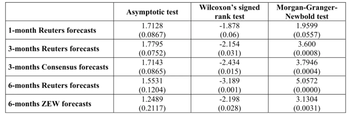
Table 2 summarizes the results for accuracy of professional exchange rate forecasts. As for all market forecasts mean errors are positive, professional forecasters tend to overestimate the future development of the Euro against the US-dollar in the considered time period. In addition, the comparison of the accuracy of professional forecasts with naïve random walk forecasts reveals that for all measures the random walk is superior to professional forecasts. This result is also approved by the Theils’s inequality coefficient that is clearly above one for all market forecasts. However, these results do not indicate whether the differences between the forecasting accuracy of market forecasts and naïve random walk forecasts are statistically significant. For this purpose we refer to three different statistical tests. In particular we apply an asymptotic test as suggested by Diebold and Mariano, [1995], the Wilcoxon’s Signed-Rank test and the Morgan-Granger-Newbold test (see for a detailed discussion of these tests Diebold and Mariano, [1995]).
Table 3: Tests of differences in professional forecast errors
Asymptotic test Wilcoxon’s signed rank test Morgan-Granger-Newbold test
1-month Reuters forecasts (0.0867) 1.7128 -1.878 (0.06) (0.0557) 1.9599
3-months Reuters forecasts (0.0752) 1.7795 (0.031) -2.154 (0.0008) 3.600
3-months Consensus forecasts (0.0865) 1.7143 (0.015) -2.434 (0.0004) 3.7946 6-months Reuters forecasts (0.1204) 1.5531 (0.001) -3.189 (0.0000) 5.0572
6-months ZEW forecasts (0.2117) 1.2489 (0.028) -2.198 (0.0031) 3.1304
Table 3 summarizes the results of statistical tests comparing the forecasting accuracy of professional exchange rate forecasters and naïve random walk forecasts. The corresponding null hypothesis consists of no differences in the forecasting accuracy of both forecasts. The results indicate that the forecasting performance of professional exchange rate forecasters are statistically significant worse than those of naïve random walk forecasts. Merely for the six month forecasts of Reuters and ZEW the asymptotic test reveals the same forecast performance for both forecasts.
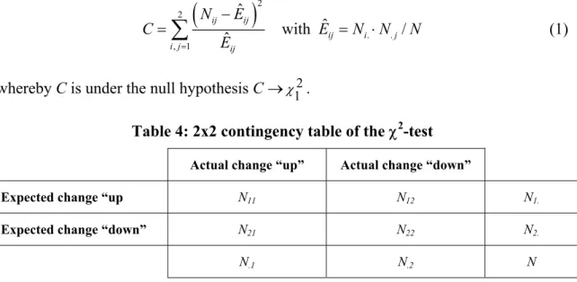
To investigate the usefulness of professional forecasts as direction of change forecasts we carry out a simple χ2-test of independence (see Diebold and Lopez, [1996]). Thereby
the forecasting quality of professional forecasts is compared to a naïve coin flip. The test is based on a 2 x 2 contingency table (see Table 4). The hit rate of the direction-of-change forecasts is given by the quotient (N11 + N22)/N. The actual exchange rate
changes are defined as “up” if ∆St+h ≥ 0 and as “down” if ∆St+h < 0. Accordingly,
expected exchange rate changes are defined as “up” if Et∆St+h ≥ 0 and as “down” if
Et∆St+h < 0. N.1 and N.2 denote the total frequency of “actual change up” and “actual
change down”. Correspondingly, N1. and N2. denote the total frequency of “expected
change up”, respectively, “expected change down”. The null hypothesis of the test is that the entries in the contingency table are completely random, so that the hit rate is close to 50 %. According to Diebold and Lopez, [1996], the corresponding test statistic is given by
(
)
2 2 . . , 1 ˆ ˆ with / ˆ ij ij ij i j i j ij N E C E N N N E = − =∑
= ⋅ (1)whereby C is under the null hypothesis C→ 2 1
χ .
Table 4: 2x2 contingency table of the χ2-test
Actual change “up” Actual change “down”
Expected change “up N11 N12 N1.
Expected change “down” N21 N22 N2.
N.1 N.2 N
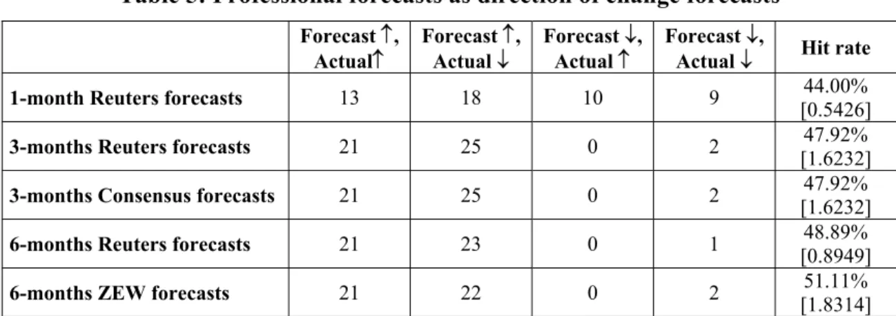
Table 5 presents the results of the χ2-test. It clearly shows that professional forecasts are poor predictors for the future direction of exchange rate changes. Only the six months forecasts of the ZEW show a hit rate slightly above 50%. However, this result is not statistically significant.3 For all other market forecasts the hit rate is well below 50%,
whereby no result is statistically significant.
Table 5: Professional forecasts as direction of change forecasts
Forecast ↑,
Actual↑ Forecast Actual ↓↑, Forecast Actual ↑↓, Forecast Actual ↓↓, Hit rate
1-month Reuters forecasts 13 18 10 9 [0.5426] 44.00%
3-months Reuters forecasts 21 25 0 2 [1.6232] 47.92%
3-months Consensus forecasts 21 25 0 2 [1.6232] 47.92%
6-months Reuters forecasts 21 23 0 1 [0.8949] 48.89%
6-months ZEW forecasts 21 22 0 2 [1.8314] 51.11%
Test-statistics are given in brackets.
Altogether, the empirical results show that the forecasting accuracy of professional exchange rate forecasts is rather low. None of the market forecasts is able to beat a naïve random walk forecast, whereby this result is statistically significant. Furthermore, professional market forecasts even fail to predict the future direction of exchange rate changes.
3 Experimental analysis of human forecasting behavior
Although the negative results for the professional exchange rate forecasts are completely in line with the empirical evidence of macroeconomic exchange rate models (see Meese and Rogoff, [1983a] and Meese and Rogoff, [1983b]), it is hard for economists to accept the unsatisfying outcome. Therefore, we decided to investigate the human forecasting behavior in an experimental environment to extract potentially important characteristics of the human forecasting behavior.
3.1 Experiment design
The experiments were conducted in 2003 at computer terminals at the Department of Economics, University of Wuerzburg and at the Department of Statistics and Operations Research, University of Graz. Overall, three experiments were run with a total of 136 undergraduate students. The subject’s task was comprised of the prediction of a time series, one-period (46 subjects), three-periods (45 subjects) and six-periods ahead (45 subjects). The size of the groups is comparable to the samples of professional forecasters. Subjects were not allowed to participate in more than one experiment. The experimental procedures were identical in all three experiments, solely the forecasting horizon varies across the three experiments. Figure 2 shows a English translation of the computer screen the participants are facing during the experiment. On the screen the subjects are informed about their own past forecasts and the actual time series up to the time of forecasting.
Figure 2: Screenshot of the computer experiment
The time series xt presented to the subjects is a realisation of an autoregressive process
of second order,
0 1 1 2 2
t t t t
x =α α+ x− +α x− +ε ,
with the coefficients α0 = 0.09, α1 = 1.19, α2 = -0.28 and the error term εt being
uniformly distributed in the interval [-5;5]. The coefficients were estimated from the US-$/€ exchange rate time series. All values have two decimal places. The first value of the experimental time series was presented to the subjects before they emitted their initial forecast. No further history of past values was presented. The time series was unlabelled and the subjects were not given any contextual or background information. Overall, the subjects made 41 forecasts. Figure 4 shows the time series xt and the
Figure 3: Experimental time series and forecasts 0 5 10 15 20 25 30 35 40 1 4 7 10 13 16 19 22 25 28 31 34 37 40 43 46 Time series xt
one step ahead forecast 0 5 10 15 20 25 30 35 40 1 4 7 10 13 16 19 22 25 28 31 34 37 40 43 46 Time series xt
three step ahead forecast
0 5 10 15 20 25 30 35 40 1 4 7 10 13 16 19 22 25 28 31 34 37 40 43 46 Time series xt
six step ahead forecast
Note: The judgmental forecasts are shifted back to the time of forecast formation.
In order to provide appropriate incentives, the subjects received payments according to their forecasting accuracy. The payments are based on absolute forecast errors and had the form
∑
t42=2max{
a f− t;0}
, where ft denotes the individual forecast and a is a constant value. The constant a was set to 30 cents in the one-step and six-step task and was set to 40 cents for the three-step ahead forecasts, in order to assure equal payments.4 The average payment across all three experiments was approximately 3 € for an average duration of about 20 minutes.3.2 Accuracy of experimental forecasts
To make the experimental forecasts comparable to the professional forecasts, we aggregated the individual forecasts of the novices in each experiment by calculating their arithmetic mean. The accuracy of the experimentally generated average forecasts is analyzed by the means of the above applied measures. Table 6 presents the results for the forecasting accuracy of judgmental forecasts. Whereas professional forecasters overestimate the time series, the negative values for mean errors indicate that the judgmental forecasts underestimate the time series in all experiments. The mean squared errors in all experiments are lower than the corresponding values of the naïve random walk forecasts. Consequently, the Theil’s inequality coefficient is below the critical value of one for all three forecast horizons. However, the judgmental forecasts are not
4 We knew from the results of pilot studies that the three-step ahead forecasting task was more difficult
than the others. The payment scheme had to be modified in order to equalize the financial rewards for all subjects.
generally superior to naïve random walk forecasts since the mean absolute errors of one- and three-step ahead forecasts are larger than the naïve benchmark. Only for the six-step ahead horizon judgmental forecasts perform better than the random walk by all error measures.
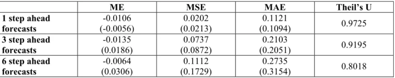
Table 6: Accuracy of experimental forecasts
ME MSE MAE Theil’s U
1 step ahead forecasts (-0.0056) -0.0106 (0.0213) 0.0202 (0.1094) 0.1121 0.9725 3 step ahead forecasts -0.0135 (0.0186) (0.0872) 0.0737 (0.2051) 0.2103 0.9195 6 step ahead forecasts -0.0064 (0.0306) 0.1112 (0.1729) 0.2735 (0.3154) 0.8018 In parenthesis are the measures for naïve random walk forecasts.
To check the results for statistical significance, we also carried out the tests for differences in the forecast errors of judgmental forecasts and naïve random walk forecasts. The results reveal that although the performance seems to be better at first glance it is not statistically significant (see Table 7). Only for the six step ahead forecasts the Morgan-Granger-Newbold test suggest a statistically significant better performance of judgmental forecasts.
Table 7: Tests of differences in experimental forecast errors
Asymptotic test Wilcoxon’s signed rank test Morgan-Granger-Newbold test 1 step ahead forecasts (0.6542) -0.4479 (0.861) -0.175 (0.6949) -0.3950 3 step ahead forecasts (0.5568) -0.5877 -1.341 (0.18) (0.1855) -1.3472 6 step ahead forecasts (0.3177) -0.9993 (0.801) -0.253 (0.0160) -2.5166
P-values are in parenthesis.
A possible explanation for the relatively good performance of judgmental forecasts may be found in the correct anticipation of the future direction of the time series. Table 11 illustrates the quality of experimental forecasts as a direction of change forecasts. However, although the one step and six step ahead forecasts show a hit rate of over 50% the results are statistically insignificant, so that it is fair to conclude that judgmental forecast are not able to predict the future direction of the time series accurately.
Table 8: Experimental forecasts as direction of change forecasts
Forecast ↑,
Actual↑ Forecast Actual ↓↑, Forecast Actual ↑↓, Forecast Actual ↓↓, Hit rate
1 step ahead forecasts 13 18 10 9 [0.563] 56.1% 3 step ahead forecasts 7 11 14 9 [1.953] 39.0% 6 step ahead forecasts 7 10 10 14 51.2% [0.001] Test statistics are given in brackets.
4 The nature of expectations
The results of section 2 and 3 have shown that professional forecasters perform worse than novices in an experimental environment. The forecasting accuracy of professional exchange rate forecasters is significantly worse than naïve random walk forecasts, whereas the novices in our experimental setting perform at least as good as the naïve forecasts. This outcome is quite astonishing as, on the one hand, novices did not possess any contextual information concerning the evolution of the time series and, on the other hand, the forecasting performance of novices is evaluated over all 41 periods, although the subjects did not knew any history of the time series and thus the forecasting task is very difficult in the first periods.
An explanation for this results may be found in the nature of expectations. Possibly, professional forecasters and novices show different characteristics with regard to their expectations that may be responsible for differences in their forecasting performance. With respect to expectations the economic literature highlights the prominence of the concept of rational expectations. According to the rational expectations hypothesis (REH), rational subjects produce unbiased forecasts by using all available information. In the following, we first evaluate the rational expectation hypothesis empirically. Afterwards, we investigate different expectation formation mechanisms which may also help us to identify important differences between professional exchange rate forecasts and judgmental forecasts of novices.
4.1 Rational expectation hypothesis
The rational expectation hypothesis implies that forecast errors of rational subjects (ξt+1)
conditioned on the available information set (Ωt) should be purely random,
(
)
(
2)
1 1 1 , with 1 ~ 0,
t St E St t t
ξ+ = + − + Ω ξ+ σ (2)
where S denotes the nominal spot exchange rate and E is the rational expectations operator. Thus, the unbiasedness hypothesis implies that under REH forecasts errors are expected to be zero, i.e. they fluctuate randomly so that ex post no systematic deviations of the actual spot rate from the expected rate should be observed. The unbiasedness hypothesis can be tested econometrically by regressing the actual change in the spot exchange rate on the expected change according to the professional forecasts. Thus, the null hypothesis of unbiasedness implies that it is possible to decompose st+h-st as
(
)
t h t t t h t t h
s+ − = +s α β E s+ −s +ε + (3) where s is the logarithm of the nominal spot exchange rate, α = 0, β = 1 and εt+h has a
mean of zero and is uncorrelated with EtSt+h-St (see Cavaglia et al., [1994], p. 327).
A second implication of the rational expectation hypothesis is that forecast errors of rational subjects are serially uncorrelated. This condition can directly be tested by estimating
1 1 2 2
t t t n t n t
The hypothesis of serially uncorrelated forecast errors implies that α = β1 =β2=…=
βn=0.
Furthermore, the rational expectation hypothesis implies that rational subjects generate their forecasts by using all available information efficiently. This implication is often called the orthogonality condition. According to the orthogonality hypothesis rational forecasts incorporate all available information, so that their predictive power can not be improved by the inclusion of any variable that is known at the time of expectation formation. Consequently, forecasts errors must be uncorrelated with any variable in the available information set. The orthogonality hypothesis can be tested by regressing the ex post forecast errors against some known information available when market participants form their forecasts,
t h t t h t t h
s+ −E s+ = +α βX +ε+ (5)
where Xt is a set of information known at time t and the orthogonality hypothesis holds
if α = 0 and β = 0. In our regression approach, the information set Xt contains lagged
exchange rates, so that the regression equation is given as
1 2 1 1
t h t t h t t n t n t h
s+ −E s+ = +α βs +β s− + +" β s− − +ε+ . (6)
4.1.1 Rationality of professional exchange rate forecasts
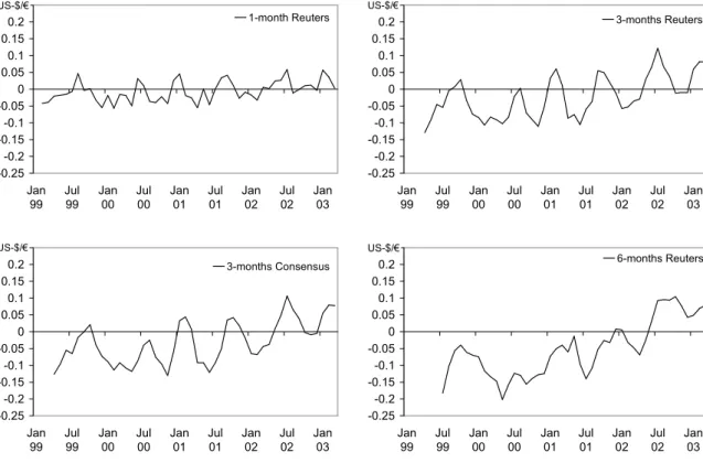
Already a simple graphical analysis illustrates that professional forecasts are difficult to reconcile with rational expectation hypothesis (see Figure 4). Instead of fluctuating randomly, the forecasts exhibit systematic deviations. Until the spring of 2002 almost all forecasts were too optimistic for the Euro; after that date they were too pessimistic.
Figure 4: Expectation errors of survey data
-0.25 -0.2 -0.15 -0.1 -0.05 0 0.05 0.1 0.15 0.2 0.25 Jan
99 Jul99 Jan00 Jul00 Jan01 Jul01 Jan02 Jul02 Jan03 US-$/€ 1-month Reuters -0.25 -0.2 -0.15 -0.1 -0.05 0 0.05 0.1 0.15 0.2 0.25 Jan
99 Jul99 Jan00 Jul00 Jan01 Jul01 Jan02 Jul02 Jan03 US-$/€ 3-months Reuters -0.25 -0.2 -0.15 -0.1 -0.05 0 0.05 0.1 0.15 0.2 0.25 Jan 99 Jul 99 Jan 00 Jul 00 Jan 01 Jul 01 Jan 02 Jul 02 Jan 03 US-$/€ 3-months Consensus -0.25 -0.2 -0.15 -0.1 -0.05 0 0.05 0.1 0.15 0.2 0.25 Jan 99 Jul 99 Jan 00 Jul 00 Jan 01 Jul 01 Jan 02 Jul 02 Jan 03 US-$/€ 6-months Reuters
-0.25 -0.2 -0.15 -0.1 -0.05 0 0.05 0.1 0.15 0.2 0.25 Jan 99 Jul 99 Jan 00 Jul 00 Jan 01 Jul 01 Jan 02 Jul 02 Jan 03 US-$/€ 6-months ZEW
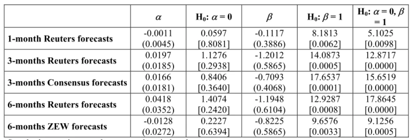
Table 9 shows the results of estimating equation (3) for each market forecast and for each available forecast horizon via ordinary lest squares (OLS). The standard errors for the three and six months market forecasts stem from applying the Newey and West, [1987] estimation procedure that allows for heteroscedasticity in the error terms.5 For an evaluation of the null hypotheses of α = 0 and β = 1, we carry out Wald Tests. Table 9 demonstrates the corresponding F-statistics. However, it must be noted that the results of the Wald Tests should be interpreted with caution as the standard assumptions with respect to the F-test are rather demanding and may not be fulfilled.
Table 9: Test of unbiasedness for the US-$/€ market forecasts
α H0:α = 0 β H0:β = 1 H0:α= = 10, β
1-month Reuters forecasts (0.0045) -0.0011 [0.8081] 0.0597 (0.3886) -0.1117 [0.0062] 8.1813 [0.0098] 5.1025 3-months Reuters forecasts (0.0185) 0.0197 [0.2938] 1.1276 (0.5865) -1.2012 [0.0005] 14.0873 [0.0000] 12.8717 3-months Consensus forecasts (0.0181) 0.0166 [0.3640] 0.8406 (0.4068) -0.7093 [0.0001] 17.6537 [0.0000] 15.6519 6-months Reuters forecasts (0.0352) 0.0418 [0.2420] 1.4074 (0.6104) -1.1948 [0.0008] 12.9287 [0.0000] 17.8645 6-months ZEW forecasts (0.0272) -0.0128 [0.6394] 0.2227 (0.5865) -0.8225 [0.0033] 9.6576 [0.0005] 9.1256
Standard errors in parentheses; p-values in brackets.
For all market forecasts the results indicate that the hypothesis of unbiasedness should be rejected. Figure 5 illustrates that the slope coefficients (β) for all professional market forecasts over all forecasting horizons are negative instead of being approximately one. Consequently, the regression results indicate that although the α coefficients are almost close to zero, the β coefficients clearly depart from one. The Wald-Tests suggest that for all market forecasts the null hypothesis of α = 0 can not be rejected. However, the null hypothesis of β = 1 and the joint hypothesis of α = 0 and β = 1 can not be maintained.
5 Hansen and Hodrick, [1980] demonstrate that, when the forecast horizon is larger than the observational
frequency, the forecast error εt+k will be serially correlated. This can be corrected by using the Newey and
West, [1987] estimation procedure (see Cavaglia et al., [1994], pp. 327). We also run all regressions by explicitly modeling the autocorrelation structure of residuals. Overall, these results coincide with the results obtained by using Newey and West, [1987] estimation procedure. The results are available on request.
Figure 5: Scatter diagrams for the unbiasedness hypothesis of professional exchange rate forecasts
-.03 -.02 -.01 .00 .01 .02 .03 .04 -.08 -.04 .00 .04 .08 e xpec te d on e m ont h chang e
actual one month change one month Reuters forecasts
-.03 -.02 -.01 .00 .01 .02 .03 .04 .05 .06 -.1 .0 .1 .2 ex p e ct ed th re e m o nt h c han ge
actual three month change three month Reuters forecasts
-.02 -.01 .00 .01 .02 .03 .04 .05 .06 .07 -.1 .0 .1 .2 e xpec ted th ree m o n th change
actual three month change three month Consensus forecasts
-.02 .00 .02 .04 .06 .08 .10 -.2 -.1 .0 .1 .2 e xpec ted s ix m ont h c hange
actual six month change six month Reuters forecasts
-.02 -.01 .00 .01 .02 .03 .04 .05 .06 .07 -.2 -.1 .0 .1 .2 e xpec ted s ix m ont h c hange
actual six month change six month ZEW forecasts
The results of testing for serial correlation in professional forecast errors also indicate that the rational expectation hypothesis must be rejected for almost all professional exchange rate forecasts. Table 10 summarizes the results of estimating equation (4) via ordinary least squares (OLS) and the corresponding Wald tests, which check for the hypothesis of α = β1 = β2=…= β4=0. Just for the one month Reuters exchange rate
forecasts the null hypothesis can not be rejected. All other professional exchange rate forecasts show serially correlated forecast errors.
Table 10: Test for serial correlation in professional forecast errors
α β1 β2 β3 β4 βH0: α = 1…β4 = 0 1-month Reuters forecasts (0.0052) -0.0044 (0.1563) 0.3085 (0.1693) 0.0001 (0.1695) -0.0231 (0.1622) -0.1832 [0.2545] 1.3742 3-months Reuters forecasts -0.0045 (0.0068) (0.1493) 1.0722 (0.2111) -0.1756 (0.2147) -0.5726 (0.1530) 0.3755 [0.0000] 20.3089 6-months Reuters forecasts -0.0016 (0.0076) 1.1892 (0.1695) -0.4043 (0.2626) 0.1223 (0.2625) 0.0153 (0.1698) 51.3124 [0.0000] 3-months Consensus forecasts (0.0070) -0.0051 (0.1482) 1.1854 (0.2265) -0.2817 (0.2297) -0.5357 (0.1531) 0.3965 [0.0000] 29.8217 6-months ZEW forecasts (0.0080) -0.0032 (0.1711) 1.1288 (0.2550) -0.3220 (0.2518) -0.0023 (0.1659) 0.0519 [0.0000] 26.7208 Standard errors are in parenthesis; p-values in brackets.
The orthogonality hypothesis is empirically evaluated by the means of estimating equation (6). Table 11 shows the corresponding results which are obtained by using ordinary least squares (OLS). The standard errors for the three and six months market forecasts stem form applying the Newey and West, [1987] estimation procedure that allows for heteroscedasticity in the error terms.6 For an evaluation of the null hypothesis
α = β1 =β2=…= β4=0, we carry out Wald tests. The corresponding F-statistics are also
summarized in Table 11.
The results for the orthogonality hypothesis are somewhat mixed. For the one-month and three-months professional exchange rate forecasts from Reuters the Wald tests indicate that the orthogonality hypothesis can not be rejected. Thus, these forecasts are in line with the orthogonaliy hypothesis. However, for the three-months Consensus forecasts and the six-months Reuters and ZEW forecasts the null hypothesis of orthogonality must be rejected.
Table 11: Orthogonality test for professional exchange rate forecasts
α β1 β2 β3 β4 βH0: α =
1…β4 = 0
1-month Reuters forecasts (0.0061) -0.0088 (0.1720) 0.2150 (0.2640) -0.3342 (0.2699) -0.0098 (0.1712) 0.0528 [0.4275] 1.0042 3-months Reuters forecasts (0.0173) -0.0412 (0.3085) -0.0499 (0.3038) -0.3238 (0.3718) -0.3639 (0.2861) 0.4324 [0.1053] 1.9666 6-months Reuters forecasts (0.0234) -0.0834 (0.4186) -0.3504 (0.4262) 0.0924 (0.3530) -0.0717 (0.3483) -0.2535 [0.0251] 2.9412 3-months Consensus forecasts (0.0180) -0.0476 (0.3182) 0.1734 (0.3019) -0.5075 (0.3923) -0.3130 (0.3149) 0.3866 [0.0733] 2.2048 6-months ZEW forecasts (0.0219) -0.0663 (0.3710) -0.7121 (0.3613) 0.3733 (0.3597) 0.1247 (0.3496) -0.3224 [0.0236] 2.9830
Standard errors in parentheses; p-values in brackets.
Overall, our results are in line with the results reported in other studies. Chinn and Frankel, [2002] analyze 24 survey forecasts of the Currency Forecasters’ Digest. They found that the unbiasedness hypothesis is resoundingly rejected. Harvey, [1999] investigated the unbiasedness hypothesis of survey forecasts for the British Pound, the Deutsche Mark, the Japanese Yen and the Swiss Franc against the US-dollar. His results also indicate a wholesale rejection of the unbiasedness hypothesis. Similar results are also reported by .e.g. Dutt and Ghosh, [1997], Sobiechowski, [1996], Cavaglia et al., [1994], Cavaglia et al., [1993] and Beng and Siong, [1993]. For the orthogonality hypothesis the empirical evidence is rather similar. Cavaglia et al., [1993] choose to include the forward premium into the information set Xt and find that the forward
premium contains additional information for exchange rate forecasts. Beng and Siong, [1993] report that forecasters could have improved their predictions of future exchange rates by better exploiting existing information. Sobiechowski, [1996] rejects the null hypothesis of orthogonality in three out of four forecast horizons. Harvey, [1999] also analyzes the orthogonality hypothesis for various exchange rates and finds a sound rejection of the hypothesis.
4.1.2 Rationality of experimental forecasts
In contrast to the professional exchange rate forecast errors, judgmental forecast errors of novices fluctuate much more randomly and show no systematic biases (see Figure 6). This visual impression is also approved by the scatter diagrams for the unbiasedness hypothesis of experimental forecasts. Unlike the professional forecasts the correlation between the expected change and the actual change appears clearly to be positive.
Figure 6: Expectation errors for experimental forecasts -15 -10 -5 0 5 10 15 1 4 7 10 13 16 19 22 25 28 31 34 37 40 43 46
one step ahead forecast errors
-15 -10 -5 0 5 10 15 1 4 7 10 13 16 19 22 25 28 31 34 37 40 43 46
three step ahead forecast errors
-15 -10 -5 0 5 10 15 1 4 7 10 13 16 19 22 25 28 31 34 37 40 43 46
six step ahead forecast errors
Figure 7: Scatter diagrams for the unbiasedness hypothesis
-.15 -.10 -.05 .00 .05 .10 .15 .20 -.4 -.3 -.2 -.1 .0 .1 .2 .3 .4 ex pec ted o n s tep ahe ad c hange
actual one step ahead change one step ahead forecasts
-.2 -.1 .0 .1 .2 .3 .4 -.8 -.6 -.4 -.2 .0 .2 .4 .6 .8 ex pec ted t h ree s tep ahead ch ange
actual three step ahead change three step ahead forecasts
-.3 -.2 -.1 .0 .1 .2 .3 .4 .5 -0.8 -0.4 0.0 0.4 0.8 1.2 ex p e ct ed si x s tep ahead c hange
actual six step ahead change six step ahead forecasts
In order to analyse statistically whether judgmental forecasts are consistent with the unbiasedness hypothesis, we ran the regression equation (3) for the judgmental forecasts of novices for all three horizons. The estimation results are summarized in Table 8. Again, the standard errors for the three-step and six-step ahead forecasts stem from applying the Newey and West, [1987] estimation procedure (see FN 5). The α coefficients do not differ significantly from zero and the β coefficients do not depart significantly from one. Thus, the results for the Wald-Tests suggest that the joint hypothesis of α = 0 and β = 1 can not be rejected for judgmental forecasts over all considered horizons so that we conclude that the unbiasedness hypothesis can not be rejected by estimating equation (3).
Table 12: Test of unbiasedness for the judgmental forecasts
α H0: α = 0 β H0: β = 1 H0: α = 0, β = 1 1 step ahead forecasts -0.0004 (0.0224) [0.9852] 0.0004 (0.3516) 0.6535 [0.3305] 0.9712 [0.6167] 0.4894 3 step ahead forecasts -0.0209 (0.0622) 0.1131 [0.7384] 0.7464 (0.7516) 0.1139 [0.7376] 0.0745 [0.9282] 6 step ahead forecasts (0.0857) -0.0513 [0.5526] 0.3588 (0.5128) 1.1173 [0.8202] 0.0523 [0.7820] 0.2474 Standard errors in parentheses; p-values in brackets.
However, the test for serial correlation in the judgmental forecast errors indicates that forecast errors are serially correlated for the three-step and six-step ahead forecasts (see Table 13). These results point to first caveats against the rational expectation hypothesis in the context of judgmental forecasts.
Table 13: Test for serial correlation in experimental forecast errors
α β1 β2 β3 β4 βH0: α = 1…β4 = 0 1 step ahead forecasts (0.0239) 0.0073 (0.1762) 0.1944 (0.1764) -0.2843 (0.1776) 0.2204 (0.1790) -0.0769 [0.5712] 0.7804 3 step ahead forecasts 0.0038 (0.0273) (0.1764) 1.1990 (0.2629) -0.8982 (0.2617) 0.3716 (0.1679) -0.0528 [0.0000] 11.4333 6 step ahead forecasts -0.0067 (0.0270) 1.3014 (0.1694) -0.8943 (0.2642) 0.7394 (0.2807) -0.3414 (0.1823) 20.7908 [0.0000] Standard errors in parentheses; p-values in brackets.
Further evidence against the rational expectation hypothesis in the context of judgmental forecasts can be obtained from the verification of the orthogonality hypothesis. The orthogonality hypothesis is empirically evaluated by the means of estimating equation (6) for the judgmental forecasts via OLS. The standard errors for the three-step and six-step ahead forecasts are again adjusted according to the Newey and West, [1987] procedure (see FN 5). The joint hypothesis of α = β1 =β2=…= β4=0
is investigated via Wald tests; the corresponding F-statistics are given in Table 14 as well.
The results reveal that for the six-step ahead forecasts the orthogonality hypothesis must be rejected according to the Wald tests. For the one-step ahead forecasts the null of orthogonality can be maintained. However, the results for the orthogonality hypothesis are quite sensitive to the size of lags included in the regression. For example, including eight lags in the regression leads to resounding rejection of the null of orthogonality.
Table 14: Orthogonality test for the judgmental forecasts
α β1 β2 β3 β4 βH0: α = 1…β4 = 0 1 step ahead forecasts 0.2203 (0.3132) (0.1907) 0.1103 (0.3118) -0.4173 (0.3137) 0.5240 (0.1911) -0.2862 [0.6593] 0.6557 3 step ahead forecasts 0.7189 (0.8195) -0.1135 (0.3440) -0.2480 (0.5063) 0.3497 (0.6009) -0.2178 (0.2693) 1.1252 [0.3664] 6 step ahead forecasts (0.5304) 1.2999 (0.4019) -0.1994 (0.3869) -0.0833 (0.3678) 0.5674 (0.3112) -0.7067 [0.0055] 4.0730 Standard errors in parentheses; p-values in brackets.
Overall, our empirical results for the rational expectation hypothesis in the context of judgmental forecasts are much more mixed compared to the results for the professional exchange rate forecasts. Whereas the first test for unbiased judgmental forecasts indicates that these forecasts are mainly in line with the concept of rational expectations, both other tests show that maintenance of the rational expectations hypothesis for judgmental forecasts is at least doubtful. This is especially true for the three-step and six-step ahead forecasts.
However, our results align with the evidence reported in previous experimental studies. In an experiment of Dwyer et al., [1993] subjects had to report one-step ahead forecasts of a pure random walk. This simple experimental setting allows the straightforward analysis of rational expectations, because rationality is clearly defined: subjects should forecast the previous observation for the next period. The forecasts were found to be unbiased and the subjects made efficient use of the available information, a results that provides support for rational expectations. In an earlier study also concerned with judgmental forecasts of pure random walks, Mason, [1988] concluded similarly. However, the majority of the authors find little support for the rational expectation hypothesis from experimental data. Schmalensee, [1976], Garner, [1982], Brennscheidt, [1993] and Hey, [1994] (to mention a few) had to reject the hypothesis of rational expectations in their forecasting experiments. Especially for describing the individual forecasting behaviour, the rational expectation hypothesis appears to be inappropriately. The consistency with rational expectations seems to depend on the task complexity, which was also considered by Dwyer et al.
Summarising the empirical evidence for the rational expectation hypothesis for professional exchange rate forecasts and judgmental forecasts, we have to state that the rational expectation hypothesis is rejected for both kinds of forecasts. However, the results show interesting differences in the characteristics of professional exchange rate forecasts and experimental forecasts of novices. Whereas the unbiasedness hypothesis has to be clearly rejected for the professional exchange rate forecasts, the judgmental forecasts of novices seem to be unbiased. According to the results of testing for serial correlation in forecast errors and orthogonality, we find no meaningful differences between professional forecasts and forecasts of novices.
4.2 Different expectation formation mechanisms?
The nature of the expectation formation mechanism may be responsible for the accuracy and rationality of forecasts. Thus, differences in the expectation formation mechanism may be an explanation for the differences between professional exchange rate forecasts and judgmental forecasts of novices. Typically, two different expectation formation mechanisms are explored in the literature. The first kind of expectation formation mechanism is called adaptive expectations. According to this expectation formation mechanism expectations are a function of current expectation errors. The second kind of expectation formation is called extrapolative expectations and captures the impact of past realization on the expectation formation.
Both expectation formation mechanism will be tested empirically against the alternative of static expectations. In this context static expectations correspond to the naïve random walk forecast. Since professional exchange rate forecasts perform statistically worse than naïve forecasts we expect that the hypothesis of static expectations must be rejected. For the judgmental forecasts of novices we expect to confirm the hypothesis of static expectations.
4.2.1 Adaptive expectations
The first kind of expectation formation is called adaptive expectations. The adaptive expectations hypothesis - or error-learning model – describes the change of the forecast as an adjustment depending on the error between the actual exchange rate and the last forecast:
(
)
t t h t h t t t h t t
E s+ −E s− = +α β s −E s− +ε (7)
The adaptive expectation hypothesis requires that α = 0 and 0 ≤β≤ 1. The case β = 1 represents the naïve forecast Etst+h= st.
4.2.1.1 Adaptive expectations of professional forecasts
The results of estimating equation (7) using professional exchange rate forecasts are summarized in Table 15. The standard errors for the three-step/months and six-step/months forecasts stem from applying the Newey and West, [1987] estimation procedure. The βcoefficients of all forecasts are significantly smaller than one except for the 1-month Reuters forecasts. The joint hypothesis of α = 0 and β = 1 has to be rejected for all forecasts although the hypothesis α = 0 has to be rejected for all forecasts. Thus the data can be interpreted as being consistent with adaptive
expectations. Overall, this result correspond largely with the existing empirical evidence on adaptive expectations in the context of foreign exchange markets (see Chinn and Frankel, [2002]).
Table 15: Test for adaptive expectations of professional forecasts
α H0: α = 0 β H0: β = 1 H0: α = 0, β = 1 1-month Reuters forecasts (0.0019) 0.0039 (0.0504) 4.0330 (0.0552) 0.9430 [0.3074] 1.0648 [0.0309] 3.746 3-months Reuters forecasts (0.0036) 0.0163 [0.0000] 21.2073 (0.0378) 0.9030 [0.0137] 6.5766 [0.0000} 24.1754 3-months Consensus forecasts (0.0046) 0.0240 [0.0000] 26.4175 (0.0437) 0.8552 [0.0000] 10.9586 [0.0000] 50.2069 6-months Reuters forecasts 0.0278 (0.0045) 37.6726 [0.0000] 0.7859 (0.0405) 27.8692 [0.0000] 37.4407 [0.0000] 6-months ZEW forecasts (0.0027) 0.0250 [0.0000] 85.4088 (0.0293) 0.9230 [0.0124] 6.9034 [0.0000] 61.7108 Standard errors in parentheses; p-values in brackets.
4.2.1.2 Adaptive expectations of judgmental forecasts
The tests for adaptive expectations reveal quite different results that were observed for professionals as it is reported in Table 16. All α coefficients are not significantly different from zero. The β coefficients are significantly smaller than one for the three- and six-step ahead forecasts, but significantly larger for the one-step ahead forecasts. This means that the hypothesis of adaptive expectations has to be rejected for the short term forecasts but can be maintained for the others. These mixed results from the adaptive model do not help to explain the differences in forecasting accuracy.
Table 16: Test for adaptive expectations of judgmental forecasts
α H0: α = 0 β H0: β = 1 H0: α = 0, β = 1
1 step ahead forecasts (0.0089) -0.0089 [0.3269] 0.9865 (0.0638) 1.2298 [0.0009] 12.9806 [0.0029] 6.8295 3 step ahead forecasts (0.0224) -0.0060 [0.7905] 0.0717 (0.0807) 0.8214 [0.0334] 4.8950 [0.0620] 3.0066 6 step ahead forecasts (0.0179) -0.0013 [0.9421] 0.0054 (0.0614) 0.5210 [0.0000] 60.8690 [0.0000] 30.8015
4.2.2 Extrapolative expectations
The second kind of expectation formation is called extrapolative expectations. According to this expectation mechanism, the expectations are affected solely by past realizations:
(
)
t t h t t t h t
E s+ − = +s α β s −s− +ε . (8) Crucial for the interpretation of this expectation mechanism is the sign of the coefficient
β. If β < 0, expectations are stabilizing in the sense that a recent movement in the exchange rate gives rise to the expectation of a reserve change in the future. Is β > 0, expectations are called bandwagon expectations. Here, forecasters expect that current exchange rate movements will recur in the future. For β = 0, forecasters have static
expectations, i.e. they expect that future exchange rate changes are independent from past exchange rate changes. Thus, they believe exchange rates follow a random walk process.
4.2.2.1 Extrapolative expectations of professional exchange rate forecasts
Figure 8 displays the scatter diagrams of the expected h-month exchange rate change versus the previous h-month change. Obviously, past exchange rate changes have a substantial impact on the expected future exchange rate changes. Thereby, the negative slope of the regression line indicates that professional exchange rate forecasters usually expect a reversal of past exchange rate movements in the future. Consequently professional exchange rate expectations can be classified as stabilizing in the above mentioned sense. The visual evidence is also confirmed by empirical analysis. For this purpose we run the regression equation (8) for all available professional exchange rate forecasts, whereby we include previous one month exchange rate changes as well as past exchange rate changes over the applied forecasting horizon. The results are summarized in Table 17.
The results of estimating equation (8) show that professional exchange rate forecasts for the one month Reuters forecasts and the 6 months ZEW forecasts considering the past one month exchange rate changes appear to be static. However, for all other expectations the regression analyzes reveals that the β coefficients are statistically significant negative, so that the hypothesis of static expectations is rejected in favor of stabilizing expectations. Consequently, professional exchange rate forecasters expect on average that the current exchange rate movement will be reversed in the future. These results are in line with the findings of Cavaglia et al., [1993] who report also negative β coefficients for professional exchange rate forecasts.
Table 17: Test for extrapolative expectations of professional forecasts
α β H0: β = 0
1-month Reuters forecasts st −st−1 (0.0020) 0.0041 (0.0678) -0.0477 [0.4848] 0.4958
3
t t
s −s− (0.0035) 0.0183 (0.0512) -0.0889 [0.0892] 3.1086
3-months Reuters forecasts
1 t t s −s− (0.0034) 0.0178 (0.1085) -0.1975 [0.0749] 3.3169 3 t t s −s− (0.0044) 0.0284 (0.0664) -0.1355 [0.0475] 4.1630
3-months Consensus forecasts
1 t t s −s− (0.0042) 0.0277 (0.1241) -0.3217 [0.0128] 6.7256 6 t t s −s− (0.0050) 0.0368 (0.0491) -0.2260 [0.0000] 21.184
6-months Reuters forecasts
1 t t s −s− (0.0059) 0.0376 (0.1524) -0.3842 [0.0152] 6.3532 6 t t s −s− (0.0023) 0.0266 (0.0247) -0.0933 [0.0005] 14.2285
6-months ZEW forecasts
1
t t
s −s− (0.0034) 0.0259 (0.1034) 0.1302 [0.2146] 1.5848
Figure 8: Expected versus previous exchange rate changes -.03 -.02 -.01 .00 .01 .02 .03 .04 -.08 -.04 .00 .04 .08 ex pec te d one m ont h change
previous one month change Reuters forecasts -.10 -.05 .00 .05 .10 .15 -.04 -.02 .00 .02 .04 .06 ex pec ted th ree m o n th change
previous three month change Reuters forecasts -.02 -.01 .00 .01 .02 .03 .04 .05 .06 .07 -.1 .0 .1 .2 ex p e ct ed th re e m o nt h c han ge
previous three month change Consensus forecasts -.02 .00 .02 .04 .06 .08 .10 -.2 -.1 .0 .1 .2 ex pec te d s ix m ont h c h ang e
previous six month exchange rate Reuters forecasts .00 .01 .02 .03 .04 .05 .06 .07 -.2 -.1 .0 .1 .2 e xpec ted s ix m ont h c hange
previous six month change ZEW forecasts
4.2.2.2 Extrapolative expectations of judgmental forecasts
In contrast to the professional forecasts, the results for the judgmental forecasts of novices is not so clear cut. The scatter diagrams of the expected h-step change versus the previous h-step change indicates that for the one step ahead forecasts a positive slope coefficient is found, so that novices form bandwagon expectations over the short forecasting horizon (see Figure 9). However, for the three-step and six-step ahead forecast the slope coefficients are again negative which implies that long-run expectations are expected to be stabilizing.
Figure 9: Expected versus previous change in the experimental time series
-.15 -.10 -.05 .00 .05 .10 .15 .20 -.4 -.3 -.2 -.1 .0 .1 .2 .3 .4 e xpec ted one s tep ahead c hange
previous one step ahead change one step ahead forecasts
-.2 -.1 .0 .1 .2 .3 .4 -.8 -.6 -.4 -.2 .0 .2 .4 .6 .8 three step ahead forecasts
ex pec ted t h ree s tep ah ead change
previous three step ahead change
-.3 -.2 -.1 .0 .1 .2 .3 .4 .5 -0.8 -0.4 0.0 0.4 0.8 1.2 six step ahead forecasts
ex p e ct ed s ix s tep ahead ch a nge
previous six step ahead change
Table 18 shows the results for estimating equation (8) for the judgmental forecasts. Again, we include previous one–step ahead changes as well as past changes over the applied forecasting horizon in the regression analysis. As expected from the visual evidence, the one-step ahead forecasts reveal a tendency for extrapolating past changes in the future. The related β coefficient is found to be statistically significant and the Wald test clearly rejects the null hypothesis of β = 0. For the three step ahead forecasts the empirical tests indicate that these expectations are static. Neither the β coefficients
are statistically significant different from 0 nor the Wald tests suggest that the null hypothesis of β = 0 must be rejected. With regard to the six step ahead forecasts, the results show a tendency that these expectations are stabilizing, although considering past one-step ahead changes indicate static expectations.
Table 18: Test for extrapolative expectations of judgmental forecasts
α β H0: β = 0
1 step ahead forecasts st−st−1 (0.0126) -0.0069 (0.0495) 0.2864 [0.0000] 33.4222
3
t t
s −s− (0.0266) 0.0050 (0.0960) -0.1086 [0.2654] 1.2798
3 step ahead forecasts
1 t t s −s− (0.0275) -0.008 (0.1365) 0.1224 [0.3753] 0.8048 6 t t s −s− (0.0385) 0.0035 (0.1105) -0.3055 [0.0092] 7.6492
6 step ahead forecasts
1
t t
s −s− (0.0452) 0.0099 (0.1911) -0.2231 [0.2502] 1.3638
Newey and West, [1987] adjusted standard errors are in parentheses.
Overall, for the extrapolative expectation mechanism we find interesting differences between professional and judgmental forecasts concerning the impact of past realizations on future expected movements. Whereas professional exchange rate forecasters predominantly expect that current exchange rate movements will be reversed in the future, judgmental forecasts of novices exhibit a structure which is consistent with the phenomena of mean reversion often observed in financial time series (see Cutler et al., [1990]). The results coincide with the results of De Bondt, [1993] who studied probabilistic forecasts of students in several experimental settings. He found evidence that novices expect a continuation of past trends, while experts expect a reversal.
4.3 Discussion of the results
Section 2 and 3 have revealed that the accuracy professional exchange rate forecasts and judgmental forecasts of novices is significantly different from one another. Therefore we decided to analyze the expectations of professional forecasters and novices in more detail to extract important differences in their expectations. Overall, we have found two remarkable differences. First, professional forecasters form predominantly regressive expectations whereas novices show a tendency to extrapolate recent trends in the short-run (one step ahead forecasts) and expect a reversal in the long-short-run (six step ahead forecasts). Second, the tests of unbiasedness show that professional forecasts are over all forecast horizons biased predictors of future exchange rates, whereas judgmental forecasts of novices appear to be unbiased.
These results may serve as advice for an explanation for the inferior forecasting accuracy of market forecasts compared to judgmental forecasts. Professional exchange rate forecasts seem to be biased by fundamental considerations as these forecasts are oriented towards the fundamental equilibrium exchange rate. Figure 10 clearly shows that professional forecasters expected for the whole period that the €/US-$ rate should appreciate towards its fundamental value in the future. Here, the fundamental value is
measured by the purchasing power parity using consumer price indices. The corresponding PPP level is around 1.20 US-$/€ and coincides largely with other estimates for the US-$/€ fundamental equilibrium rate (see Table 19). Overall, the phenomena of an expected convergence towards the fundamental exchange rate is more distinctive the longer the forecast horizon is. However, Figure 10 also reveals that professional forecasters do not expect an immediate adjustment of the actual exchange rate to its fundamental level. Professional forecasters rather assume that current exchange rates only move gradually towards the PPP level. The sluggishness in the expected exchange rate movements, although it seems reasonable at first glance, clearly contradicts the predictions of the efficient market hypothesis. According to the efficient market hypothesis, deviations of the actual exchange rate from its fundamental justified level evoke speculative trading activities of rational market participants that bring the actual exchange rate directly towards its fundamental value (see Friedman, [1953]).
Table 19: Selected estimates for the US-$/€ fundamental equilibrium rate
Reference period Equilibrium exchange rate (US-$/€)
Wren-Lewis and Driver (1998) 2000 1.19 – 1.45
Borowski and Couharde (2000) 1999 (first half) 1.23 – 1.31
Clostermann and Schnatz (2000) Winter 1999/2000 Medium-run: 1.13 Short-run: 1.20
Chinn and Alquist (2001) June 2000 Medium-run: 1.17 – 1.24
Lorenzen and Thygesen (2000) 1999 Long-run: 1.28
Goldman Sachs (2000) May 2000 1.21
Source: Schneider, [2003], European Central Bank, [2002]
Rationales for expecting a sluggish adjustment to the fundamental rate expectations can be found in the reasons for the rejection of the efficient market hypothesis. Contrary to the efficient market hypothesis, foreign exchange markets are dominated by heterogeneous traders which follow – at least partially – irrational trading practices such as technical analysis, bandwagon expectations and herding (see Menkhoff, [1998], Cheung and Chinn, [2001]and Gehrig and Menkhoff, [2004]). These trading practices may be responsible for long-lasting deviations of the actual exchange rate from its fundamental level and may cause that adjustments towards that level occur – if at all – only gradually. Thus, it is quite reasonable for professional forecasters to expect that the adjustment to the fundamental level does not occur in an abrupt manner but sluggishly. A further explanation for sluggish expectations with respect to the adjustment to PPP levels can be found in the representativeness heuristics (see Kahneman et al., [1999]). According to this heuristics, subjects tend to believe that past movements of exchange rates are representative for the data generating process of the exchange rate itself and it is likely that similar movements will recur in the future. Thus, professional forecasters assume that the speed of adjustment towards the fundamental level is limited by the usually observable exchange rate movements.
Figure 10: Professional exchange rate forecasts and fundamental exchange rates 0.8 0.85 0.9 0.95 1 1.05 1.1 1.15 1.2 1.25 1.3 Jan
99 Jul99 Jan00 Jul00 Jan01 Jul01 Jan02 Jul02 Jan03
EUR/USD 1 months Reuters PPP exchange rate 0.8 0.85 0.9 0.95 1 1.05 1.1 1.15 1.2 1.25 1.3 Jan
99 Jul99 Jan00 Jul00 Jan01 Jul01 Jan02 Jul02 Jan03
EUR/USD 3 months Reuters PPP exchange rate 0.8 0.85 0.9 0.95 1 1.05 1.1 1.15 1.2 1.25 1.3 Jan 99 Jul 99 Jan 00 Jul 00 Jan 01 Jul 01 Jan 02 Jul 02 Jan 03 EUR/USD 3 months Consensus PPP exchange rate 0.8 0.85 0.9 0.95 1 1.05 1.1 1.15 1.2 1.25 1.3 Jan 99 Jul 99 Jan 00 Jul 00 Jan 01 Jul 01 Jan 02 Jul 02 Jan 03 EUR/USD 6- months Reuters PPP exchange rate 0.8 0.85 0.9 0.95 1 1.05 1.1 1.15 1.2 1.25 1.3 Jan 99 Jul 99 Jan 00 Jul 00 Jan 01 Jul 01 Jan 02 Jul 02 Jan 03 EUR/USD 6 months ZEW PPP exchange rate
Note: the fundamental exchange rate is calculated according to the purchasing power parity using consumer price indices. As starting point for the calculation of the fundamental exchange rate we use the actual exchange rates at the time of the Louvre Accord in February 1987.
To assess the suggestion of fundamental-biased professional exchange rate forecasts, we compare these forecasts with artificial fundamental-oriented forecasts. We decided to approximate the fundamental value of the €/US-$ exchange rate by the purchasing power parity condition (PPP) as it is an adequate long-run equilibrium exchange rate model (see Sarno and Taylor, [2002]). Furthermore, we incorporate an inertia factor that accounts for the sluggishness of expectations. We assume that the artificial fundamental-oriented forecasts predict an appreciation of the €/US-$ rate if the current rate is below its fundamental value and a depreciation if the current rate is above its fundamental value:
(
)
(
)
if : S 1 if : S 1 t t t h fund t t h t t t h S S E S S S α α + < + = > − (9)where St is the fundamental equilibrium exchange rate measured by the purchasing
power parity and αh denotes an inertia factor. The values for the inertia factor αh vary
with the forecast horizon and are deduced from the mean absolute exchange rate changes over three different forecast horizons; i.e. α1 = 0.02, α3 = 0.05 and α6 = 0.06.
Figure 11 illustrates the professional exchange rate forecasts and the corresponding artificial fundamental-oriented forecasts calculated according to equation (9). Both kinds of forecasts show akin characteristics. This visual impression is also assured by