Master thesis
2015
Does debt make you rich? - An empirical study of the effect
leverage has on stock-returns
Authors: Rickard Kotte Supervisor: Maria Gårdängen Gustav Lind
Abstract
Debt is commonly used by firms as a way of financing. Factors driving stock return have been the subject of numerous studies. Investors are constantly seeking ways to better understand stock return, which is where financial statements may provide them with relevant information. The presented research paper focuses on explaining whether there is a significant relationship between stock return and leverage (as well as its components). Furthermore, the authors investigated whether changes in tax and the tax shield deriving from interest bearing debt can significantly affect the stock return. The panel dataset contains quarterly observations
between 2000-2015 of the non-financial firms listed on Nasdaq OMX Stockholm’s mid-cap list. By studying a different market than the commonly researched U.S. market and
highlighting the interest-bearing portion of the debt carried by firms, the authors shed new light on the topic of leverage. By integrating a number of factors of interest into one study (instead of, as commonly done, studying one factor) the authors provide a different approach to the study of leverage in the context of the Miller and Modigliani’s framework, thus
providing new insights.
The authors have statistically shown that an increase in leverage has a negative impact on the stock return. The findings furthermore showed correlation between the stock return and the debt parameters, as well as the presence of abnormal returns during tax rate decrease.
Keywords: Leverage, stock return, Swedish stock exchange, debt, tax shield, tax rate, Miller & Modigliani, trade-off theory, mid-cap, interest bearing debt
TABLE OF CONTENT
Abstract ... 2
Chapter 1: Introduction ... 5
1.1 Background of the Study ... 5
1.2 Problem Discussion ... 6
1.3 Problem Statement ... 7
1.4 Research Objectives ... 7
1.5 Disposition ... 8
Chapter 2: Literature Review ... 9
2.1 Introduction ... 9
2.2 Capital Structure: Miller & Modigliani Framework ... 9
2.3 Trade-‐off Theory ... 11
2.4 Leverage: Does it affect stock return? ... 12
2.5 Hypotheses ... 14
Chapter 3: Methodology ... 16
3.1 Methodological approach ... 16
3.2 Methodological Theories ... 17
3.2.1 Panel data ... 17
3.2.2 The Hausman Specification Test: Fixed Effects or Random Effects? ... 20
3.2.3 Event Studies and the Market Model ... 20
3.3 Regression models ... 22
3.3.1 Test variables ... 23
3.3.2 Control variables ... 24
3.4 Criticism towards the methods used ... 27
3.4.1 Validity ... 27
3.4.2 Reliability ... 28
3.5 Delimitations ... 29
Chapter 4: Analysis and Discussion ... 30
4.1 Introduction ... 30
4.2 Hypothesis H1A: How does leverage affect stock return? ... 31
4.3 Hypothesis H1B: How does debt affect stock return? ... 33
4.4 Hypothesis H2A: How does the tax shield affect stock return? ... 36
4.5 Hypothesis H2B: How does a decrease in tax rate affect stock return? ... 37
5.1 Summary of the Results ... 39
5.2 Recommendations for Further Research ... 43
Bibliography ... 45
Chapter 1
Introduction
This section provides a brief background on the topic of the research. The authors furthermore discuss the problem, state the purpose of the study and the matters treated. The authors conclude the chapter by presenting the disposition of the study in order to give the reader a synopsis.
1.1 Background of the Study
Over the last century financial markets have grown to become one of the key drivers of the economy in modern society. With its’ roots in the industrial revolution, stock markets enabled companies to early on find financing, and with an increasing number of firms the importance of stock markets grew. Even though there are other ways to raise capital than debt, debt markets are more common tools for financing than equity (Jegadeesh, Henderson, & Weisbach, 2006).
With debt-markets having grown three-fold and stock markets with 35% between 2000 and 2013 (World Gold Council, 2014) (Appendix B), it is evident that corporations are becoming more reliant on the financial markets. During recent decades many markets have experienced an increase in corporate debt levels. During the 2000’s the euro area was experiencing a rapid increase in debt levels up until the financial crisis, after which debt levels were stabilized (European Central Bank, 2014), whilst corporate debt levels in the U.S. have continued growing rapidly (Cox, 2014). One of the explanations to high corporate debt levels may be, as shown by Graham, Lemmon & Schallheim (1998), high corporate tax rates.
With stock markets having become a global phenomenon, investors are exposed to both internal (firm specific) factors as well as external (macroeconomic) factors affecting the return. As information (such as financial statements) is easier to access, the financial markets of today have capacity to react faster than before. With external factors lying outside of a firm’s sphere of control, what firms themselves can do to affect stock return is especially important.
1.2 Problem Discussion
Starting from the late 1950’s, when Merton Miller and Franco Modigliani (1958, 1959) opposed earlier notions by stating that capital structure is irrelevant in perfect market conditions, several studies have been made on the effects of capital structure. Studies that followed added violations (such as tax) to the original framework and examined the role of capital structure in value creation. There are many factors influencing the choice of capital structure. They range from those that are observable to external audience (such as tax exposure), to those that are not (e.g. management style). When firms' have decided to increase the amount of debt in the capital structure, value creation can be reached by interest deductions that counteract tax expenses. (Fama & French, 1998)
Most of the existing empirical studies on the relationship between capital structure, tax effects and stock return, such as Cai & Zhang (2011) and Masulis (1983), have focused on the U.S. market. Besides limited research on non-U.S. markets, most studies are fragmented, only studying the effects of a single variable (e.g. leverage) and/or its components (e.g. debt). Not only are the results obtained in previous research inconclusive, they also contradict each other. Therefore, the need for further investigation is evident. Both from a market perspective (with focus on other markets than the U.S.) and from an integration perspective (joining leverage and tax in one study).
There is one more issue worth discussing; as pointed out by Welch (2011), roughly half of recent studies on leverage define leverage incorrectly. By incorporating non-financial liabilities, non interest-bearing debt is wrongly included in the leverage measurement. This final observation addresses the need to renew and clearly define leverage ratio.
Studying the Swedish stock exchange will add to the scope of academic research on leverage and its effect on stock return. The interest in studying the Swedish market lies in that it is one of the leading financial markets in northern Europe, that at the same time has not been the object of many studies in general, and leverage in particular. By studying the Swedish market and focusing on an interest-bearing leverage measure, the study will therefore provide academic and practical value.
1.3 Problem Statement
This study examines the relationship between firms’ leverage (and its components) and stock return. It furthermore attempts to examine the effects, if any, that change of corporate tax rates may have on stock return. The study analyses the prior literature written on the topic and discusses the resulting empirical findings. The authors conduct a quantitative study on the matter and elaborate on the findings. Finally conclusions and implications are presented. The main question of the research is the following: How do firm leverage and its components affect stock returns?
Due to the legitimate relationship between leverage and taxes in the theoretical framework, the study will moreover examine whether there is an observable relationship between change in statutory corporate tax rate and stock return.
1.4 Research Objectives
The principal objective of the study is to analyze the relationship between firms’ leverage (and its components) and their stock return. It furthermore investigates the relationship between tax rates and stock return.
In order to achieve this, the authors deem it necessary to follow the following steps:
First, critically analyze previous literature and discuss the research approaches, methodologies and the results of the empirical findings of the studies.
Secondly, create a method to test the hypotheses of the study.
Thirdly, analyze and discuss the results obtained from the study conducted.
Ultimately, present conclusions based on the findings in the previous analysis, suggest implications for both theory and practice as well as propose areas for further research.
1.5 Disposition
Chapter one is the introduction to the study. It provides the background of the study, as well as highlights the problems of the research. It finally formulates the objectives of the study and the steps necessary to be taken in order to reach the objectives. Furthermore the introduction provides the discussion of the academic and practical significance of the study.
Chapter two contains the literature review. In the literature review the theories on which the study is based are presented and defined. The authors use the literature review as a base where theories, definitions and main concepts are identified, as well as the previous research made on the topic of the study.Finally, the hypotheses that are tested in the study are formulated. Chapter three contains the methodology that the authors have used in their study as well as discloses the thoughts behind the chosen approach. The chapter provides insights in how the data was gathered and used along with pointing out the delimitations made. It is concluded with a critical discussion towards the methodology chosen for the study.
Chapter four presents the findings of the study along with the analysis and authors’ interpretation. The main objective of this chapter is to provide the results of the hypotheses’ tests and to eventually answer the main problem discussed in the introduction.
Chapter five concludes the study. The authors present a summary of the main findings of the study. The chapter also provides suggestions for practical and academic implications and recommendations.
Chapter 2
Literature R
eview
In the literature review the authors present theories on capital structure and leverage, as well as present previous studies on related topics. In addition, the authors present the theories, models and the vocabulary used in the study. Finally, the hypotheses of the study are presented.
2.1 Introduction
This literature review is dedicated to present the theoretical framework (base) and vocabulary that the authors will use throughout the study. The first part describes the basic theories on capital structure by Miller and Modigliani (M&M from hereafter) and its role in corporations. It continues by providing a presentation of relevant theoretical frameworks built from the original M&M’s theory. The final section presents the reader with previous research made on the topic of this study, i.e. leverage’s effect on stock return, and discusses their results.
2.2 Capital Structure: Miller & Modigliani Framework
The greatest theoretical breakthrough regarding capital structure, which up to this day shapes our view of it, was the framework made by M&M during mid 20th century. They created propositions, the first being the irrelevance proposition (proposition I); in essence, a perfect market where the value of the firm would not be affected by capital structure, but rather by earning power and asset risks (Herczeg, 2014). In order to create this environment, Miller & Modigliani (1958, 1959) made four main assumptions:
• Homogeneous expectations • Homogeneous business risk • Perpetual Cash flows
• Perfect capital market
With homogeneous expectations M&M imply that all market participants share information. All value-relevant information is available to all actors in the market, which is used to
determine the value of a security (Ogden, Frank, & O'Connor, 2002). In the basic framework of Miller & Modigliani (1958), firms are classified into homogenous business risk classes where firms in the same class have the same level of financial risk. The perpetuity of cash flows leads to investors being aware of a firm’s investment program, and once a capital structure is chosen it is fixed. Consequently this means that the operations and strategies are fixed and known by all investors (Ogden, Frank, & O'Connor, 2002). The last assumption is the assumption regarding a perfect capital market. In a perfect capital market the investors are rational and trade without restrictions, all participants borrow and lend on same terms, the capital markets are efficient whilst transaction and bankruptcy costs as well taxes are not present (Ogden, Frank, & O'Connor, 2002).
In reality, however, the assumptions are of course not valid and have therefore been further discussed. The imperfection of taxes and the role that corporate taxes play is addressed by Miller & Modigliani (1963) as well as by Miller (1977). They show that when corporate tax is present the optimal capital structure for a firm maximizing its value is one fully debt financed (100% debt) (Herczeg, 2014).
M&M’s second proposition deals with the Weighted Average Cost of Capital (WACC) and states that as a firm’s debt increases, the return on equity also increases in a linear fashion. The more debt a firm carries, the higher risk premium is demanded from its investors due to an increase in risk (Miller & Modigliani, 1958). In the first scenario, where tax is not present, the leverage ratio does not affect a firm’s WACC. The reason to why the WACC is unaffected is that the firm’s capital structure is irrelevant, as shown in proposition I.
When adding the dimension of corporate tax to the discussion, tax savings from the interest deduction are recognized which in turn reflects in a negative relationship between WACC and portion of debt carried (Miller & Modigliani, 1958).
2.3 Trade-off Theory
The main foundation of the trade-off theory is based on the framework established by Miller & Modigliani (1958), which suggests that one can obtain a higher value of the firm by adding debt to the capital structure. According to their first proposition the market value of the firm is independent from the leverage ratio (Ogden, Frank, & O'Connor, 2002). Despite these conclusions their second proposition states that expected return on firm’s equity will increase due to a higher leverage. An increase in risk is similarly an increasing function of a higher leverage (Ogden, Frank, & O'Connor, 2002).
With these propositions in mind a modification can be made to show how the trade-off theory explains an increase in the value of the firm. The increase in firm value derives from the tax shield obtained by increasing the amount of debt carried. The tax shield can be explained as the annual reduction in taxes due to interest deductibility(Ogden, Frank, & O'Connor, 2002). Thus tax shield originating from interest costs is the difference between the amount of tax paid without debt in the capital structure and the taxes paid with debt present (Wrightsman, 1978).
The following formula is modified from proposition 1:
𝑉! = 𝑉!+𝑃𝑉 𝑡𝑎𝑥 𝑠ℎ𝑖𝑒𝑙𝑑 = 𝑉!+𝜏!𝐷 (1)
Where VL and Vu are the values of the leveraged and unleveraged firm respectively, 𝜏!𝐷 is the corporate tax-rate
multiplied by the firm’s debt. This term is considered to be the firms tax shield.
As seen in equation 1, the value is no longer independent of the choice of capital structure and tax advantages can be obtained by adding debt.
As the financial leverage increases, by adding debt, the value of the firm will increase proportionally due to a larger tax shield. Since the corporate tax rate is independent from the leverage, the tax shield increases at the same rate as the debt does (Wrightsman, 1978).
In this case a firm should aim for an optimal debt level, which would allow them to acquire full tax advantages. The optimum is determined at the point where the marginal tax effect is equal to the marginal cost of leverage (DeAngelo & Masulis, 1980).Ultimately this means that by maximizing firm’s debt, the value of the firm is likewise maximized (Wrightsman, 1978).
A higher leverage (due to more debt in the capital structure) leads to an increase in expected financial distress and bankruptcy costs (Andrade & Kaplan, 1998). Since different firms are experiencing different tax rates and different rates of expected cost of future financial distress/bankruptcy costs, the optimal capital structure may vary across firms. The limited amount of debt a firm can carry in its capital structure is dependent on how much the distress costs will increase from adding debt (Ogden, Frank, & O'Connor, 2002). Kane, Marcus & McDonald (1984) do however find that although important, bankruptcy costs are not the only important variable that determines capital structure.
In conclusion, the advantages from interest deductibility will work as a counterpart to the distress costs, and increase the value of the firm. This will happen when a firm reaches their optimal debt level and the tax shield (𝜏!𝐷) will be larger than the distress costs (Kane,
Marcus, & McDonald, 1984).
2.4 Leverage: Does it affect stock return?
Leverage can be defined as the sensitivity of the equity ownership value, in regards to changes in the firm’s underlying value as argued by Welch (2011). Since the paper presented by Titman & Wessels (1988), proposing six ways of measuring leverage, several new measurements have emerged.
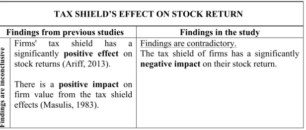
Only few previous studies have specifically tested for the effects that the (change in) tax and tax shield may have on firms’ stock return. However, by testing leverage ratio’s effect on stock return one is indeed incorporating the tax shield (tax shield being a function of debt). Despite the lack of studies made on this particular topic, Graham, Lemmon, & Schallheim (1998) find a positive relationship between corporate tax rate and the amount of debt firms carry.
Earlier studies have shown significant effects on the stock return due to changes in leverage. Studies focusing on the relationship between stock return and leverage do however have different approaches. A common subject is to look at changes in volatility due to a change in the leverage. This is referred to as the leverage effect and is beyond the scope of this study. Cai & Zhang (2011) present a general approach in their study, examining if changes in leverage have any effect on the stock price. The authors use U.S. data and find a negative effect on the stock return stemming from an increase in leverage in the previous quarter. The
effect is more likely to be found in companies that suffer from debt overhang, yet it can also appear in financially healthy firms. Both measurements of leverage used in the study have total liabilities in the numerator, but differ by having total assets and market equity in the denominator respectively. The findings are especially interesting since they oppose the basic theory previously presented.
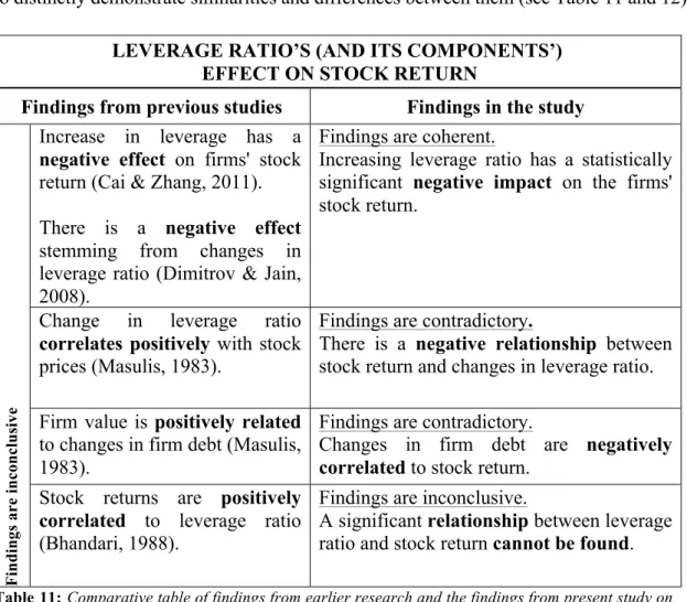
The results presented by Cai & Zhang (2011) are consistent with the study conducted by Dimitrov & Jain (2008). Studying U.S. stocks, Dimitrov & Jain (2008) confirm that a change in leverage will have a negative effect on the value of the firm. Change in leverage can therefore be a useful variable to understand economic performance of firms according to the authors of the article. Although having coherent results, Dimitrov & Jain (2008) measure leverage differently from Cai & Zhang (2011). In their study, Dimitrov & Jain (2008), measure leverage as total debt (long-term debt plus short-term debt) divided by total assets. However, as argued by Welch (2011) this is not an appropriate measurement of leverage since its converse includes non-financial liabilities, which consequently are counted the same as equity. This may or may not affect validity negatively (Welch, 2011).
The results above are however not conclusive and studies such as Masulis (1983) on U.S.
stocks present contradicting results, showing positive correlation between stock return (prices)
and changes in leverage ratio. Masulis (1983) furthermore finds a positive relationship
between firm value and changes in firm debt, and also concludes that there is a positive impact on firm value from the tax effect of debt financing. These findings are coherent with the theoretical framework earlier explained in this chapter.
In comparison to the studies above, leverage can also be seen as a proxy for the risk that generates a risk premium (here tested as a proxy for beta) as in the study conducted on U.S. stocks by Bhandari (1988). Bhandari (1988) argues for beta being a valid variable to measure risk and if not, leverage might be good proxy. The results show that stock returns are positively correlated with leverage ratio but not because it is a proxy for beta. They also show that the premium associated with higher leverage doesn’t seem to be a sort of risk premium. In Bhandari’s (1988) study, leverage is measured by subtracting total equity from total assets (equals total debt) and dividing it with market value of equity. Even though the same leverage measurement is included in Cai & Zhang’s (2011) study, their results contradict each other. Some previous studies have also evaluated at the median leverage ratio for a certain industry. These types of studies examine what will happen if firms deviate from the industry median.
Hull(1999) investigated whether the value of U.S. stocks is influenced during announcements of increased leverage (defined as book value of total debt divided by market value of equity), which moves away form the industry median. The result of this event study, where the event denotes the announcement period before and after the announcement of the new leverage, is that stock returns will be more negatively affected when moving away from industry norm than if firms moved closer to it.
In his study, Ariff (2013) addresses the same topic and uses the same approach as Hull (1999), but studies the phenomenon on the ASX (Australian Securities Exchange). By looking at the industry leverage ratio the study discusses whether the industry median might be a suitable proxy for the optimal capital structure. The findings, as found by Hull(1999), show a positive market reaction to leverage levels closer to industry norm. Moving away from industry median indicates a less positive or negative abnormal return. Similar to this study, Ariff (2013) also investigates the effect from tax shield by using different methods. However, out of the tests conducted a significant result was only found in one, displaying a positive relationship to stock return. Ariff (2013) concludes that the (lack of significant) results may be due to the complex tax situation in Australia and the tax obligations concerning dividends.
2.5 Hypotheses
Following the discussion above, the authors have deducted four hypotheses, which will form the base for this study. Due to the inconclusive and contradicting findings made by previous studies, the authors have decided to use a two-tailed approach.
In order to answer the problems discussed and stated in the introduction, the authors have structured the hypotheses into two main groups; H1X, focusing on capital structure (leverage and its components), and H2X, concentrating on the tax effects (tax shield and tax rate). Each hypothesis examines the relationship between the tested factor(s) and stock return. In order to crosscheck the results, the authors use two or more regressions on each hypothesis.
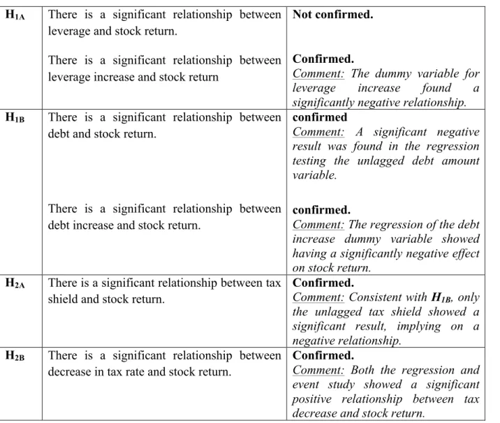
The first hypothesis from the first group, H1A, states that there will be a significant relationship between leverage ratio (increase) and stock return. The variables tested are the leverage ratio and the leverage ratio increase. This hypothesis is deducted from the previous studies showing negative relationships, when theory does suggest the opposite. The fact that there are contradicting studies on this topic is furthermore a big point of interest.
The second hypothesis, H1B, tests, in general terms, the debt’s effect on stock return. According to the hypothesis H1B, stock returns are significantly affected by debt (increase). The variables tested in the hypothesis are the amount of debt carried and the debt increase. The interest in studying the debt is that it is in fact, according to theory, the debt level and not the leverage ratio per-say that drives firm value.
Hypothesis H2A, being the first hypothesis directly examining the effects of taxes, states that the tax-shield has an observable effect on the stock returns. This hypothesis is derived from the M&M’s framework presented previously in this chapter, and unlike most studies takes a direct approach to the tax shield.
The final hypothesis, H2B, elaborates on hypothesis H2A, stating that the change in statutory corporate tax rate itself has a significant effect on the stock returns, i.e. if a decrease in statutory tax rate results in significant changes in stock returns. This hypothesis binds together previous hypotheses and is derived from the study made by Graham, Lemmon & Schallheim (1998), showing differences in capital structure (debt carried) depending on the tax rate.
Chapter 3
Methodology
In this chapter the authors describe how the study has been made. The basic frameworks and theories behind the methodology chosen for the study are presented and described. The data material used in the study is explained and the structuring of it is presented. The chapter is concluded with discussions on the reliability and validity of the study, followed by criticism towards the methods used as well as the delimitations of the study.
3.1 Methodological approach
The choice methodological approach for the study depends on the problem statement and purpose of the study. The authors’ aim is to test current theories rather than to design new ones, which leads to the use of a hypothetical deductive method. The deductive approach is a process-chain of reasoning starting from a theory or hypothesis to the empirical observations made, from which the conclusions finally are drawn (Vanderstoep & Johnston, 2009). In essence, the goal of the empirical findings from a deductive method is to support or oppose existing theories and hypotheses made on the topic (Holme, Solvang, Fløistad, Kjeldstadil, & O'Gorman, 1997).
Given that the phenomenon researched is described numerically and not in a narrative fashion, the authors have chosen to use a quantitative approach. The quantitative study consists of quarterly observations of 66 firms gathered between the years 2000 and 2015. The firms that have not been listed for the entire period are still part of the dataset. By using quarterly instead of yearly data, more variation in the time series can be observed. However since some financial variables (such as ROA) are only available on an annual basis, these variables are considered to be constant throughout all four quarters. With a time series of 60 quarters both periods of deep recession and high economic growth are covered.
Due to the subject of this research, financial firms are not included in the dataset. The key reason for this decision is that a high leverage is interpreted differently for financial firms (normally a higher leverage ratio than non-financial firms) (Fama & French, 1992). The
choice of not including financial firms is a well-used method, by e.g. Cai & Zhang (2011), Barber & Lyon (1997) and Lemmon, Roberts & Zender (2008).
The Swedish stock exchange has not been the object of many previous studies. Since Sweden is an open economy highly dependent on global trade, its stock market is highly interesting. Furthermore the Nasdaq OMX Stockholm attracts a lot of foreign investments. This combined with a high level of transparency, may indicate it to be a highly functioning market. The observable tax rate changes during the 2000’s makes Sweden a both suitable and interesting object for study.
The firms noted on the mid-cap list have in general fewer operations abroad and therefore have less complex capital structures (both in terms of macro-factors such as changing FX-rates, and in terms of identifying desired data from financial statements). Another important aspect behind the choice of mid-cap firms is that generally, by investing in the mid-cap list one is exposed to higher credit risk than that from large-cap. Consequently, a stronger reaction to changing leverage is expected to be observed.
Ultimately, the authors have chosen to use a 95% confidence interval throughout the study. The significance level is therefore equal to 5%, meaning that all the p-values equal to or smaller than 0.05 will be considered statistically significant with 95% accuracy and vice versa (Celsi, Hair, Money, Samouel, & Page, 2011).
3.2
Methodological Theories
3.2.1 Panel data
Financial modeling can sometimes be structured where both the cross-section and time series are included. This is done by structuring the dataset into a panel. Panel data is structured to measure different variables for entities (individuals) over a certain time period. Structuring data in panels allows more complicated datasets to be tested and analyzed (Brooks, 2014). The main advantages of using panel data, according to Baltagi (2005) are:
- Controlling for individual heterogeneity
- More information in the data set, more flexibility, less risk of collinearity between variables - Easier to study “dynamics of adjustment”
Panel data can either be balanced or unbalanced. To distinguish if the data set is balanced or not observations need to be made in both cross sectional and time series. If the numbers of observations in the time series is the same for each cross sectional unit it is considered to be a balanced panel data. If the numbers differ – it is unbalanced. The data can be handled as a pooled regression where all the data, both cross sectional and time series observations, is placed into a single column. Once this is done, it is easier to implement the OLS method to test the data. A pooled regression has its disadvantages when assuming that the average values of all the variables are constant both cross-sectionally and over time (Brooks, 2014).
Our dataset is considered to be unbalanced since returns are missing in the time series. The gaps in the dataset are explained by some firms being only recently listed on the stock exchange.
There are two types of effects models that are used in panel data estimations: fixed effects and random effects models. Depending on the data, different methods are appropriate for use in the panel data regressions.
In the fixed effects a disturbance term (𝑢!") is considered to affect the dependent variable (𝑦!") cross-sectionally in different ways depending on the entities. The disturbance term is defined as:
𝑢!" = 𝜇! +𝑣!" (2)
Where 𝜇! is the individual specific effect and 𝑣!" is the time varying disturbance term.
It is important to remember that 𝜇! remains constant over time. This model (which is called the Least Squares Dummy Variable (LSDV) approach) can be shown as a function of different dummy-variables, which are different depending on the entity.
𝑦!" =𝛽𝑥!"+𝜇!𝐷1+𝜇!𝐷2+𝜇!𝐷3+...+𝜇!𝐷𝑁+𝜐!" (3) For the first entity D1 is 1 and 0 for all other dummies. Using this equation one can test whether pooled regression is suitable for the dataset.
It is also possible to have a fixed effects model in the time series (Brooks, 2014).
The random effects model has different intercepts for different entities, and the intercepts being constant over time. The big difference with the fixed effects is that the intercept for every cross-sectional entity is affected by another intercept (𝛼) that affects every entity. What varies cross-sectionally is a random term (𝜖), which in this case will show the heterogeneity
across the entities. Heterogeneity can be defined as the variation in the cross-sectional element (in the LSDV fixed effects model the dummy variables show the heterogeneity). The following equation explains how the random effects works in Panel data:
𝑦!" =𝛼+𝛽𝑥!"+𝜔!" where 𝜔!" = 𝜖! +𝜈!" (Brooks, 2014) (4) Both mentioned models are ways to address endogeneity problems, which can be described as correlation between the explanatory variable and the error term. Once the regression suffers from endogeneity problems, the estimation of parameters and inference will be biased. There are three causes of endogeneity (Roberts & Whited, 2012):
1) Omitted variables; 2) Simultaneity;
3) Measurement errors (Roberts & Whited, 2012).
Omitted Variables are the variables, which are included in the error term and can explain the dependent variable, yet are left out from the regression equation (Brooks, 2014). Roberts & Whited (2012) points out that omitted variables only become an issue when they are correlated with the explanatory variables. Simultaneity issues arise when the explained and explanatory variables are functions of each other. Ultimately, measurement errors occur when variables are difficult to observe and measure. It is common to use a proxy when measurement error is a problem. (Roberts & Whited, 2012).
This study only uses fixed effects cross-sectional models. What effects models to use is decided by a Hausman test, which will be explained in the next section. The use of fixed effects in leverage studies is recommended by Lemmon, Roberts & Zender (2008), suggesting that better results for regression coefficient estimates are obtained this way.
Prior to running regressions and tests on the panel data, the dataset has been structured in excel. All the regressions and tests have thereafter been conducted using eViews. The panel data has been tested for: stationarity (using unit root test), showing stationary results; and non-linearity (using Ramsey’s RESET method), implying linearity. The results from the unit root test are shown in Appendix E.
3.2.2 The Hausman Specification Test: Fixed Effects or Random Effects?
While using panel data has many advantages, in order to study an empirical phenomenon, one needs to decide if to use a fixed effects model or a random effects model. Whether to use one or the other depends on the correlation between the unit effects and the independent variables (Bole & Rebec, 2013). The standard test to distinguish which model to use is the specification test developed by Hausman (1978).
Hausman’s (1978) specification test essentially suggests to compare 𝛽GLS and 𝛽Within which
are both consistent with the null hypothesis when H0: E(uit | Xit) = 0 is true, but with 𝛽GLS
being inconsistent when H0 is false (Baltagi, 2005).
The absence of correlation between the independent variable(s) and the unit effects means that estimates of β should be similar for both fixed effects and random effects models. Hausman test statistic H (given in the equation below) is therefore a comparison between the two (Clark & Linzer, 2012).
H = (𝛽RE −𝛽FE)’[Var(𝛽FE) – Var(𝛽RE)]-1(𝛽RE − 𝛽FE) (5)
If the two variables are significantly different, H0 is rejected, implying that the fixed effects
model should be used, and vice versa.
The authors will not elaborate further on the technicalities or practicalities of the Hausman test; if the reader has further interest in the model, the authors recommend to read Hausman (1978), Nakamura & Nakamura (1981) and Clark & Linzer (2012).
The Hausman tests in this study, conducted prior to running the regressions, all suggest the use of fixed effects models. The results of the Hausman tests are presented in appendix C.
3.2.3 Event Studies and the Market Model
An event study is, as the name suggests, a study of how a certain identifiable event impacts a financial variable (usually stock return) (Brooks, 2014). There are several empirical models to measure and estimate abnormalities (abnormal return) around (or due to) an event. Amongst those are the constant mean return model, CAPM and the Market Model (MM), the latter will be presented below (for more information on other models the authors recommend MacKinlay (1997)).
The first step when conducting an event study is to define and identify the event itself and the period under which the financial variable will be examined (the event window) (MacKinlay, 1997). If the tax-shield is a de-facto attribute, which the market takes into account while pricing a stock, one may expect an observable change in price (return) when the statutory tax changes. In order to further analyze the role of corporate tax rate in stock returns, the authors have chosen to conduct an (excel based)1event study of the corporate tax decrease in Sweden implemented in January 2013. The event window is defined and consists of quarterly observations during one year (the event year, 2013). The reasoning behind using a one-year event window is that changing tax-rates may lead to structural changes that may take time to implement (such as seen in Graham, Lemmon & Schallheim (1998)).
The next step is to determine the selection of data to use (the selection criteria). The event study conducted uses the same data as in the panel-data regression discussed earlier. Some firms in the event study have been removed due to the authors’ criteria of using full observations in the estimation and event window used.
Abnormal return is calculated by subtracting the expected normal return from the actual return (see equation 6).
𝐴𝑅!" =𝑅!"−𝐸[𝑅!"] (Brooks, 2014) (6) Since variation of the returns across the periods in the event window is likely, using the cumulative average return (CAR) may be used (see equation 7) (Brooks, 2014).
𝐶Â𝑅! 𝑇!,𝑇! = !! Â𝑅!"
!!!! (7)
This means that in order for (cumulated) abnormal return to be calculated, the normal return model needs to be estimated. Therefore the next step is to choose performance model, deciding on and defining the estimation window (the period from which the normal return parameters are estimated) and to calculate the expected normal return for the event window (MacKinlay, 1997). As mentioned previously, there are several models which all measure normal return differently. The study uses the market model. The market model assumes a stable linear relation between the market return and the return of the variable studied (Brooks, 2014).
The market model is therefore defined as the following:
Rit = α + βiRmt + εit (8)
E[εit = 0] var(εit) = 𝜎!!!
Where Rit is security i’s return at period t, Rmt is the market return at period t, εit the zero mean error term and α,
β and 𝜎!!! are the model’s parameters.
The market model’s parameters are estimated by using a regression and the expected return is calculated by inserting the actual market return for period t. The market model does therefore relate the return of any given security to the market return. Once the expected (normal) return is calculated and the (cumulated) abnormal return is obtained, the final step is to test whether or not the abnormal returns are significantly different from zero (MacKinlay, 1997). The test for significance is done by calculating the p-value of the (cumulative) abnormal returns.
3.3 Regression models
In this section the authors present and explain how the study’s regression models are developed. The section contains a discussion starting with the test- and control variables and culminates in how the reduced form regression equation is constructed.
The dependent variable in all of the regressions is stock return. The stock returns have been obtained by first extracting the quarterly stock prices from Datastream. The natural logarithm has thereafter been taken from the prices, after which the return has been calculated by subtracting the previous period’s logarithmic price from current period’s logarithmic price (see equation 9).
𝑅!" =ln (𝑆𝑡𝑜𝑐𝑘!!)− ln (𝑆𝑡𝑜𝑐𝑘!!!!) (9)
Where 𝑅!" is stock return for quarter q and 𝑆𝑡𝑜𝑐𝑘!! is stock price at quarter q.
Information may not be available to the market before the time of the announcement. In order to try to capture the de-facto change caused by the variable (e.g. leverage ratio), in some regressions all variables except the test variable(s) are lagged (i.e. the effect from Q1 announcement may not be observable before Q2). This is simulated by moving the test variable(s) “one step forward” in time (from this point on called lagged regressions).
3.3.1 Test variables
In order to solve the problem discussed in the introduction, the authors have chosen a selection of seven variables to test. In order to test the first hypotheses group, H1X, which
concerns the effect of the capital structure, the variables leverage ratio, leverage increase, debt, debt dummy and debt increase dummy are used. To assess a possible tax effect in H2X, in addition to the event study, regressions are made with the variables tax shield and tax decrease dummy. The data for the (calculations of the) test variables in group H1X has been collected by retrieving quarterly financial reports from the Thomson Reuters EIKON database. The tax rate has been collected from the OECD tax database.
Leverage ratio. Leverage ratio is in this study defined as the book value of interest-bearing debt divided by the book value of equity. The non interest-bearing debt has been manually filtered out and removed by analyzing the quarterly statements of the sample firms. Since it is the book values of debt the authors have access to, the book value of equity is used in order to be consistent. The choice of using only interest-bearing debt has been made on the basis of the theoretical framework earlier presented. Non interest-bearing debt will by definition not provide any tax-shield; hence, the removal of it is deemed necessary.
Leverage increase. The leverage increase variable is a dummy variable used to measure the effect that an increase in leverage ratio has on stock returns. If the leverage ratio has increased over the previous period, the value “1” is assigned, if no change or a decrease is observed it is given the value “0”.
Debt. As mentioned above, the debt used in this study is filtered out from non interest-bearing debt. The two debt-positions considered are long-term (interest-bearing) debt, and current portion of long-term (interest-bearing) debt. The natural logarithm is thereafter taken.
Debt Dummy. The debt dummy simply indicates whether or not a firm at time t carries debt or not. It acts as a test on, whether firms carrying (or starting to carry) debt have significantly different stock returns. If debt is present in the firm’s capital structure the number “1” is assigned, and a “0” if it is not.
Debt Increase Dummy. The debt increase dummy indicates whether or not an increase in debt has taken place between quarter q-1 and q. Value “1” signifies an increase in debt, whilst a “0” indicates an unchanged or decreased amount of debt. This variable examines the effect that an increase in debt may or may not have on stock return.
Tax Shield. The tax shield variable is used to examine the relationship between the tax shield and stock return. This variable is used due to it being the de-facto value driver of firms in the M&M’s framework. The tax shield is calculated by multiplying the, at the period, statutory corporate tax rate with the debt present. The logarithm is thereafter taken from the figures obtained.
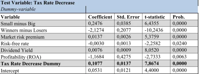
Tax Decrease Dummy. Besides testing the tax effect by an event study, a tax decrease dummy is used in the regression. During the period chosen, two tax changes have taken place (decrease in 2008 and decrease in 2013). The dummy variable is given the value “1” during the year that the decrease happened and a “0” otherwise. A full year is chosen since a tax change is a significant event and activities started as a response may take time to be implemented (e.g. taking in more debt).
3.3.2 Control variables
Structural form
The discussion regarding what drives the stock return is vast and is a research topic in itself. Given that stock return can be affected by several factors, the choice of correct control variables is of uttermost importance. Initially when creating the regression equation, several firm specific factors were chosen to be controlled for; Size, Profitability, Intangible Assets and Dividend Yield. The Fama & French (2012) five European developed market factors were furthermore chosen as factors due to their proven relevance.
Firm size is often mentioned as an important factor to explain stock return. Due to the choice of firms and different asset structures within the sample, firm size is defined as the natural logarithm of firm turnover in Swedish krona, rather than natural logarithm of asset value. The quarterly turnovers are collected from the financial statements gathered from Thomson Reuters EIKON, and the logarithm is thereafter taken.
Profitability and Dividend Yield are two more accepted drivers in explaining stock return. The authors have chosen to define profitability as the firms’ return on assets (ROA). ROA measures the profitability in terms of firms’ assets and is calculated by dividing net income by total assets. The dividend yield used is defined and expressed as a percentage of the stock price per share. The ROA and dividend yields are collected yearly and quarterly from Datastream.
The fourth firm specific control variable chosen is Intangible Assets. This factor was chosen due to many firms acting in industries where intangibles are of great importance (such as pharmaceutical patents etc.). The factor is defined as the natural logarithm of the book value of intangible assets excluding goodwill. The data regarding intangible assets is extracted from quarterly reports from Thomson Reuters EIKON.
In addition to the firm specific variables, the Fama & French (2012) five European developed market factors were used. The factors contain portfolios of firms, which are sorted by:
– Size (defined by the market cap): big (B) and small (S).
– Value (defined by the book-‐to-‐market equity): growth (G), neutral (N) and value (V).
B-firms represent the top 90% of the market cap, whereas S-firms are the bottom 10%. Similarly, G represents the bottom 30%, N – the middle 40% and V – the top 30% (Fama & French, 2012). The factors are collected from the data library of Kenneth R. French (French, 2015).
The factors are:
Market risk premium (Rm-Rf) is the excess return; the difference in return between the market and the risk-free asset.
Small minus Big (SMB) is created by producing six portfolios; three portfolios containing B-firms (BG, BN and BV) and three portfolios containing S-B-firms (SG, SN and SV). The SMB factor is the equally weighted average return of the S portfolios minus the equally weighted average return of the B portfolios.
High minus Low (HML) is in essence the V minus G return. HMLS is calculated by taking SV
– SG whilst HMLB as BV – BG. HML is then defined as the equally weighted average of the
two HMLX returns.
Winners minus Losers (WML). The return of the best performing stocks minus the return for the worst performing stocks. The portfolios are created as with HML, but using the cumulative return instead of B/M to categorize; losers (L) are the bottom 30%, neutral (N) the mid 40% and winners (W) the top 30%. WMLis defined as the equally weighted average of WMLS and WMLB.
Risk-free rate. The final factor is the risk-free rate, defined as the Swedish one-month governmental bond. The one-month bond is used in order to keep consistency with the Fama & French methodology. The risk-free rate is collected from the Swedish central bank’s homepage.
The structural form (full form) regression equation is therefore given by:
𝑅!" =𝛼+𝛽!𝐶𝑉! +𝛽!𝐶𝑉!+⋯+𝛽!𝐶𝑉! +𝛽!𝐶𝑉!+𝛽!𝑇𝑉! (10)
Where 𝑅!" is stock return for firm i at time t, 𝐶𝑉! are the control variables and 𝑇𝑉! are the test variables.
Reduced form
From the structural form the authors have created a reduced form regression equation to shield from possible issues and from using non-relevant factors. By running the regression with the control variables only, several observations were made.
The first observation made is that the firm specific variable controlling for size (ln turnover) is not significant. The reason for this is most likely that the element of size is also controlled for in the SMB factor. Including the firm specific size variable in the regression equation would therefore lead to collinearity issues within the model. The authors have therefore removed the firm specific size factor in the reduced form.
The two variables ‘HML’ and ‘Intangible Assets’ are highly insignificant in the regression, and were shown to barely add any explanatory information (next to zero difference in R2).
Based on these observations, the two variables have also been removed in the reduced form regression equation.
The reduced form regression equation is therefore given by:
𝑅!" =𝛼+𝛽!𝐶𝑉! +𝛽!𝐶𝑉!+⋯+𝛽!𝐶𝑉! +𝛽!𝐶𝑉!+𝛽!𝑇𝑉! (11)
3.4 Criticism towards the methods used
In an empirical quantitative study a bigger sample usually translates to better results. The study is limited to the Nasdaq OMX Stockholm mid-cap list. The exclusion of financial firms has further decreased the sample size to 66 firms. The sample can be considered small and by using for instance all non-financial firms listed on the Swedish stock exchange (not only mid-cap) would increase sample size considerably. A larger sample would likely provide more accurate results, on the expense of data processing needing substantially more time. Furthermore, although a stronger market reaction to leverage and leverage changes may be observable for mid-cap firms, there is a possibility that the higher credit risk yields different results than of those from a study conducted on e.g. the large-cap list.
The data set consists of an unbalanced panel meaning that full observations (i.e. starting q1 2000 and finishing q4 2014) are missing for some firms. This may have an effect leading to different results due to a biased sample.
As shown by Graham, Lemon & Schallheim (1998), firms adapt their capital structure to the tax rate. Given that changes in statutory corporate tax rates are in general announced in forehand, firms may start reacting to it long before the actual implementation of the new tax rate. It should therefore be interesting to define the event as the announcement rather than the implication, and examine changes occurring prior to the actual change.
3.4.1 Validity
Validity describes whether the researcher actually measures the phenomenon, which in the context of the study is relevant (McKinnon, 1988). Validity can therefore be expressed as the absence of systematic measurement errors (Lundahl & Skärvad, 2009). The validity of a study is compromised when the researcher’s conduct and/or design unintentionally studies more or less than the focus of the study (McKinnon, 1988).
In order to limit the noise from other variables, each hypothesis has been broken down into several regressions. By deconstructing the key question and testing the effect of the building blocks (individual variables), the authors try to isolate the relevant elements for the study; hence increasing construct validity.2
To address the problem discussed, the study distinguishes between non interest-bearing debt and interest-bearing debt, and uses only the latter. The two types of debt have been separated manually from the financial statements collected. The financial statements are regarded as reliable, and the validity of the sorted data is therefore considered to be high. However, would accounting principles allow big variation in how to book debt (interest-bearing), errors may occur.
3.4.2 Reliability
Reliability is concerned with whether or not the data that the researcher obtains is reliable (McKinnon, 1988). One may therefore define it the absence of random errors in the study, i.e. the trustworthiness of the study (Lundahl & Skärvad, 2009). High reliability insures a high consistency of a measurement. Three common categories of reliability are:
1) Quixotic reliability, observing to what extent a measurement (measured repeatedly) yields unvarying (inaccurate) results;
2) Diachronic reliability, or the stability over time;
3) Synchronic reliability, similarity of observations within a specified time period (Kirk & Miller, 1986).
The data in the study is obtained from reliable sources and the measurements used are deducted from theoretical and empirical findings. In combination with using data processing methods and software ensuring correct results, the risk of obtaining systematically inaccurate results, as portrayed in quixotic reliability, is considered low.
Due to the nature of the data studied, the diachronic reliability of the results is considered to be low. The factors affecting stock return and the weight that the market participants place on the leverage and/or its components could be somewhat predictable in the short run, but impossible to predict in the long-term.
The study being quantitatively numerical in nature, synchronic reliability of the study is not deemed relevant to further discuss by the authors.
Finally since all the hypotheses are interconnected, if the hypotheses test will show consistency and absence of contradictory results it will serve as further proof of the results reliability.
3.5 Delimitations
Due to reasons previously explained in this chapter (e.g. limited research), the data sample has been limited to firms on the Swedish stock exchange. The extraction of the necessary data from the financial statements demands a thorough analysis of certain posts in the balance sheets. Since firms do not report their debt in an identical manner, manual treatment of the data is a required. Due to the time constraints, the authors have limited the data sample to mid-cap firms.
The study is consistent in using the book values of debt and equity. The choice of using book values has been made to keep the same units (book values) in the numerator and denominator. The market value of debt is very hard to observe, and therefore the assumption is that the market values equal the book values.
What the firms do with the portion of interest-bearing debt carried/taken is hard to determine. However, due to the fact that it is interest-bearing debt, the assumption that the debt is invested in value creating activities is made. Debt may of course be used for a numerous amount of purposes, e.g. cover costs and make dividend pay-outs (controlled for in regression); the actual reasons are not taken into account.
As it was elaborated in the critical discussion, the firms’ activities responding to the change in statutory tax, are assumed to begin when the new tax rate is implemented (e.g. 1st of January). This assumption has been made due to simplification reasons, since the period where firms’ activities start may be hard identify.
Finally, the study only takes traditional tax shield into account, i.e. the tax shield deriving from interest-bearing debt. Firms’ non-debt tax shield (e.g. depreciation)3 is therefore not taken into consideration in the study.
3 For deeper discussions regarding the non-‐debt tax shield, the authors recommend Titman & Wessels (1988) and DeAngelo & Masulis (1980).
Chapter 4
Analysis and Discussion
This chapter presents the hypotheses discussed in chapter 2 and the tests conducted to answer whether they are to be confirmed or rejected. The authors furthermore present and analyze the results of the tests made and discuss the findings. The discussion culminates in a consensus regarding the answer to the main question of the study.
4.1 Introduction
By using the methods identified in chapter 3, in this chapter the authors analyze the dataset and test the previously proposed hypotheses. The results are presented, discussed and analyzed. The regressions presented in this chapter are the reduced-form equations.
The hypotheses have been structured into two main groups. The first group of hypotheses, H1X, concerns the effects that firms’ capital structure has on stock returns. It is tested by examining the calculated leverage ratio, and the dummy variable “leverage increase”. To eliminate the equity part of the leverage ratio, the second half of group H1X isolates and examines the debt’s effect on stock return.
The second group of hypotheses, H2X, adds the dimension of taxes into the discussion. Since theory suggests the value increase being an effect that stems from the tax shield, H2X focuses on the taxes’ effect on stock return. The hypotheses are tested by examining the effects on stock return originating from 1) firms’ tax shields and 2) the change in statutory tax rate. An evaluation of whether firms’ calculated tax shields and tax changes have significant relationships to stock return is made. This is done by conducting a regression analysis and by making an event study.
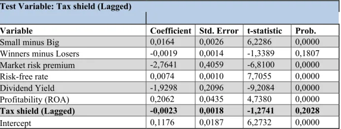
4.2 Hypothesis H
1A: How does leverage affect stock return?
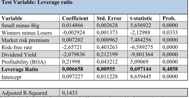
According to the first hypothesis, H1A, the authors test the statement that the leverage ratio has a significant impact on stock return. In this regression for H1A the Hausman test shows that a fixed effects model should be used. For a full view of the Hausman tests made, see Appendix C. The results from the regression are shown in the Table 1 below.
Test Variable: Leverage ratio
Variable Coefficient Std. Error t-statistic Prob. Small minus Big 0,014866 0,002628 5,656922 0,0000 Winners minus Losers -0,002924 0,001373 -2,12988 0,0333 Market risk premium 0,007202 0,000962 7,484256 0,0000 Risk-free rate -2,65721 0,403263 -6,589275 0,0000 Dividend Yield -2,079836 0,212199 -9,801364 0,0000 Profitability (ROA) 0,21998 0,043212 5,09069 0,0000 Leverage Ratio 0,006658 0,00955 0,697144 0,4858 Intercept 0,097227 0,011228 8,659445 0,0000 Adjusted R-Squared 0,1433
Table 1: Results from the first regression for H1A, testing the variable ‘Leverage Ratio’.
The results show a p-value of 0,4858 which implies that leverage has no significant effect on the stock return. Note that the variable “leverage ratio” matches the periods of the stock return (i.e. Q1 leverage ratio at Q1 stock return).
Although the adjusted R2 is rather low, creating a model which has a high explanatory power of stock return, is problematic since there are many factors which may explain stock return. The aim of the study is to measure the impact of certain factors rather than finding a suitable model, therefore the R2 values are not further discussed.
If the market does not have any information regarding the leverage ratio prior to the announcement day, the effects will not be observable before the next period. Table 2 shows the results from the lagged regression, measuring the effect in stock return at time t from the leverage ratio announced at time t-1.
Test Variable: Leverage Ratio (Lagged)
Variable Coefficient Std. Error t-statistic Prob.
Small minus Big 0,0164 0,0026 6,2200 0,0000
Winners minus Losers -0,0017 0,0014 -1,1899 0,2342 Market risk premium 0,0074 0,0010 7,7377 0,0000
Risk-free rate -2,7870 0,4037 -6,9030 0,0000
Dividend Yield -1,9947 0,2100 -9,4976 0,0000
Profitability (ROA) 0,2122 0,0434 4,8929 0,0000
Leverage Ratio (Lagged) 0,0051 0,0094 0,5477 0,5840
Intercept 0,0963 0,0112 8,5704 0,0000
Table 2: Results from the second regression for H1A, testing the lagged variable ‘Leverage Ratio’.
As with the first regression where stock return was not lagged, the lagged regression in the table 2 shows no significant effect in stock return from the leverage ratio. From the results of the two regressions presented above, it can therefore be concluded that there is no observable effect of lagged leverage ratio on stock return. The null-hypotheses of these two regressions are not rejected.
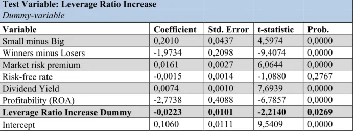
The third regression test for H1A contains the dummy variable “leverage increase”, which tests if an increase in leverage ratio significantly affects the stock returns. By just testing the leverage ratio, no significant results were obtained (see Table 1 and 2). However, with a p-value of 0,0269, the increase in leverage is found to be significant at a 95% confidence interval. This leads to the conclusion that there is an observable relationship between an increase in leverage and stock returns.
Test Variable: Leverage Ratio Increase
Dummy-variable
Variable Coefficient Std. Error t-statistic Prob.
Small minus Big 0,2010 0,0437 4,5974 0,0000
Winners minus Losers -1,9734 0,2098 -9,4074 0,0000
Market risk premium 0,0161 0,0027 6,0644 0,0000
Risk-free rate -0,0015 0,0014 -1,0880 0,2767
Dividend Yield 0,0074 0,0010 7,6939 0,0000
Profitability (ROA) -2,7738 0,4088 -6,7857 0,0000
Leverage Ratio Increase Dummy -0,0223 0,0101 -2,2140 0,0269
Intercept 0,1060 0,0111 9,5409 0,0000
The coefficient of the dummy test variable ‘Leverage Ratio Increase’ is negative, which implies that there is a negative correlation between stock return and increased leverage ratio. When a firm increases its leverage, the one period stock return will decrease. The increase in leverage can either come from changing capital structure by increasing debt or by decreasing equity where the latter falls outside the scope of this study. The relationship observed may be explained by the increased credit risk (decreased distance to default). One could argue that due to the increased credit risk, the market would expect a higher risk-premium and thereby a positive return. The authors will not discuss the aspect of risk-premium further and refers to studies made on that topic for further analysis. What is noticeable in the regression is the low standard error of the test variable, suggesting the coefficient being expected to be precise on average i.e. there is a low degree of uncertainty.
In conclusion, the results from the regression tests of H1A, show that the leverage ratio itself does not have any significant explanatory power in relation to stock return. However, what the regressions do show is that the increase in leverage ratio has a significant impact on the stock returns. This goes in line with Cai & Zhang’s (2011) and Dimitrov & Jain’s (2008) findings, in the sense that increased leverage does have a negative impact on stock return.
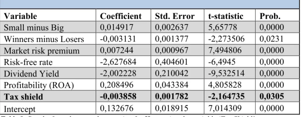
4.3 Hypothesis H
1B: How does debt affect stock return?
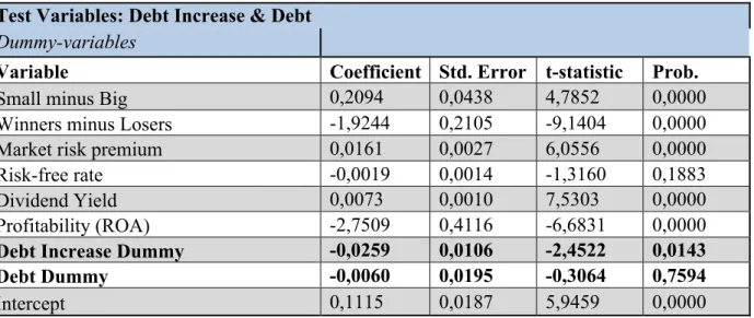
There are two ways of how the leverage ratio can be changed; either by changing firm debt, or by changing book-equity. Because of this, changes in book equity may in the data sample have an unwanted (for this study) effect on leverage ratio. In order to further analyze the debt’s effect on stock return, two dummy variables are introduced in the first regression for H1B: the “debt dummy” and the “debt increase dummy”.
In Table 4, the results of the regression with the two test variables (marked in bold) are presented. The debt dummy explains whether or not a firm at time t carries debt. The p-value for the variable is shown to be not significant. There is therefore no observed link between the stock return and whether the capital structure does or does not include debt.
Test Variables: Debt Increase & Debt Dummy-variables
Variable Coefficient Std. Error t-statistic Prob.
Small minus Big 0,2094 0,0438 4,7852 0,0000
Winners minus Losers -1,9244 0,2105 -9,1404 0,0000
Market risk premium 0,0161 0,0027 6,0556 0,0000
Risk-free rate -0,0019 0,0014 -1,3160 0,1883
Dividend Yield 0,0073 0,0010 7,5303 0,0000
Profitability (ROA) -2,7509 0,4116 -6,6831 0,0000
Debt Increase Dummy -0,0259 0,0106 -2,4522 0,0143
Debt Dummy -0,0060 0,0195 -0,3064 0,7594
Intercept 0,1115 0,0187 5,9459 0,0000
Table 4: Results from the first regression for H1B, testing the dummy variables ‘Debt’ and ‘Debt Increase’.
The results for the ‘Debt Increase Dummy’ variable (see Table 4) show whether or not there is an increase in carried debt from the last observed period. It is therefore tested whether there is an effect from an increase in debt on stock return. The p-value of 0,0143 indicates that there is a significant connection between stock return and debt increase, leading to the rejection of the null-hypothesis. Based on the value of the coefficient, it can be determined that an observed increase in debt results in a negative impact on stock return. Hence, it can be concluded that the two elements have a negative correlation. The low standard error suggests a low degree of uncertainty in the coefficient estimate.
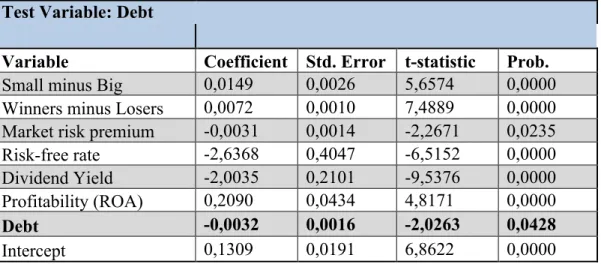
By studying the effect of the natural logarithm of the debt amount carried (note that this is the unlagged regression) on stock return, a significant relationship is observed (see Table 5). An interesting observation is that the coefficient for the test variable ‘Debt’ is negative. This combined with a low standard error, gives the estimate a low degree of uncertainty. Even though the coefficient estimate is still negative, it is noticeably higher than the one obtained for the “debt increase dummy” (see Table 4 and 5). This can be interpreted as the market putting greater emphasis on the increase of debt rather than on the (amount of) debt itself.