SOURCES, CYCLING, AND FATE OF ORGANIC MATTER IN LARGE LAKES: INGISHTS FROM STABLE ISOTOPE AND RADIOCARBON
ANALYSIS IN LAKES MALAWI AND SUPERIOR
A DISSERTATION
SUBMITTED TO THE FACULTY OF THE UNIVERSITY OF MINNESOTA BY
BRITTANY RUTH KRUGER
IN PARTIAL FULLFILLMENT OF THE REQUIREMENTS FOR THE DEGREE OF DOCTOR OF PHILOSPHY
ADVISORS: ELIZABETH C. MINOR AND JOSEF P. WERNE
i
ACKNOWLEDGMENTS
I extend my most sincere gratitude to my co-advisors; without their
encouragement, guidance, and support I am certain this would not have been possible. Liz, thank you for sharing your passion for science with me and encouraging me to be the best scientist possible at all times. Joe, thank you for your constant optimism and
unwavering excitement for science. You are both brilliant scientists and I have been inspired by you both from the very beginning of my higher education. Thank you for affording me the opportunity to learn from you both for so many years. I am forever grateful to each of you for your steadfast support during both scientific and personal trials.
I would also like to acknowledge the support and encouragement from my committee members, Dr. Tom Johnson, Dr. Donn Branstrator, Dr. Jim Cotner, and Dr. Steph Guildford. Each of you are truly excellent scientists and excellent people, and I feel very lucky to have had the support and guidance that I did from each of you, personally and professionally. Further acknowledgment is due to the open and supportive community of scientists at the Large Lakes Observatory. It is a rare
opportunity to have so many excellent scientists in such a collaborative and encouraging environment, and I feel blessed to have completed my education there. Finally, thank you a thousand times over to all the peers I was lucky enough to have along the way for the good times and support, the late nights in the lab and the great memories. To Melissa Berke and Prosper Zigah- ‘thank you’ doesn’t come close to expressing my gratitude for your mentorship and your friendship.
Heartfelt acknowledgment is also due to the world class research institutions of the National Ocean Sciences Accelerator Mass Spectrometry (NOSAMS) facility at Woods Hole Oceanographic Institute (WHOI), and the Japan Agency for Marine-Earth Science and Technology (JAMSTEC). Without the ability to travel to these incredible institutes much of the data in this dissertation would not have been possible. Particular thank you to Dr. Ann McNichol at the NOSAMS facility and to Dr. Naohiko Ohkouchi at JAMSTEC for welcoming me to visit your lab groups and perform sample analyses that
ii
would otherwise not have been possible, and to Dr. Yoshito Chikaraishi for the extensive guidance and teaching.
Finally, thank you to my parents, Rita and Jim Rowland, for their constant support and encouragement throughout my education. Thank you to my sister, Michelle Larson, and all my family, friends, and loved ones who also provided constant love and support. This wouldn’t have been possible without knowing you were standing behind me
throughout.
Major funding for this research came from the Petroleum Research Fund and SeaGrant. Additional funding and research-travel opportunities were provided by the NOSAMS graduate student internship program, the Elsevier/Organic Geochemistry Research Scholarship, the EAOG Travel Scholarship, the Butler and Jessen award, the Kerry Kelts Award, and the WRS Travel Grant.
iii
SOURCES, CYCLING, AND FATE OF ORGANIC MATTER IN LARGE LAKES: INGISHTS FROM STABLE ISOTOPE AND RADIOCARBON ANALYSIS IN
LAKES MALAWI AND SUPERIOR Brittany Ruth Kruger
Abstract
Organic matter (OM) in lake systems is sourced from in situ aquatic primary production (autochthonous), land based plant primary production or detrital material that ultimately originated from photosynthesis (allochthonous), or resuspension of organic rich sedimentary material that was ultimately sourced from a combination of all such sources. Studying the stable and radioisotopic signature of multiple chemical
components of lacustrine OM can help elucidate which of the above is the dominant OM source to the lake, as well as how OM is incorporated into and cycles through lake systems. The high organic content and biodiversity in large lakes of the world make them excellent sites to investigate such questions, and this dissertation focuses on such questions in Lake Malawi (SE Africa), and Lake Superior (North America). In Lake Malawi, the organic carbon (OC) recently deposited (within the last 50 years) is largely dominated by aquatic input, and the influence of terrestrial riverine inputs dissipates as distance from shore and water depth increase. This confirms that parameters typically used to investigate historic lake levels (and thereby to infer past climates) can in fact function as robust indicators of distance from shore, and thereby lake level. This is supported by bulk and compound specific stable carbon isotopic and radiocarbon analysis of multiple sediment fractions. Most fractions exhibited isotopic signatures nearshore that were distinct from more offshore, open-lake locations. In Lake Superior, compound specific nitrogen isotope analysis (CSNIA) of specific amino acids from species
occupying all levels of the food chain showed that Limnocalanus macrurus, a copepod, occupies a trophic level much higher than expected from known feeding habits, which may indicate the consumption of additional or unique food sources. Bulk radiocarbon
iv
analysis of the same suit of species from that lake showed Diporeia, a benthic amphipod, consumes an aged carbon source that does not appear to be significantly incorporated by other (more pelagic) organisms in this study, which rely primarily upon recently
v
Table of Contents
List of Tables……… viii
List of Figures………... ix
Chapter 1: Introduction... 1
1.1Organic Matter in Lake Systems ………... 1
1.2 Radiocarbon- genesis and application as a biochemical tracer………... 3
1.3 Focusing Research on Large Lakes………. 4
1.4 Lake Malawi……… 5
1.4.1 Modern Physical, Chemical, and Hydrologic Characteristics ………. 5
1.4.2 Geologic Setting and Historic Lake Levels……….. 8
1.4.3 Primary Production and Biota……….. 9
1.5 Lake Superior……….. 11
1.5.1 Physical, Chemical, and Hydrologic Characteristics……… 11
1.5.2 Geologic Setting and Historic Lake Levels ………. 13
1.5.3 Primary Production and Biota……….. 13
1.6 Dissertation outline……….. 15
Chapter 2: Characterizing sediment compositional change with water depth and distance from shore in a tropical rift lake……… 17
2.1 Introduction………. 17
2.2 Methods………... 18
2.2.1 Sediment Collection………. 18
2.2.2 Sediment Analyses……… 19
2.3 Results and Discussion……… 21
2.3.1 Si:Ti ………. 21
2.3.2 Elemental and Isotopic Analysis……….. 23
2.3.3 Water Content, Grain Size, and Sedimentation……… 26
2.3.4 Diatom Relative Abundance………. 28
vi
Chapter 3: Sources and cycling of Lake Malawi organic carbon: insights from
multi-fraction stable isotope and radiocarbon analyses of sediments……… 38
3.1 Introduction………. 38
3.2 Methods……… 41
3.2.1 Sediment collection………. 41
3.2.2 Lipid extraction………. 42
3.2.3 Compound isolation and radiocarbon analysis………. 43
3.2.4 Additional Fraction Analyses………. 45
3.2.5 Water column ………. 45
3.3 Results ……… 46
3.3.1 Bulk elemental analysis and biomarker relative abundance……… 46
3.3.2 Multi-fraction stable carbon isotope……… 47
3.3.3 Multi-fraction radiocarbon ……….. 47
3.4 Discussion……… 48
3.4.1 Bulk elemental analysis and biomarker relative abundance………. 48
3.4.2 δ13C of multiple sediment fractions……….. 51
3.4.3 Radiocarbon signatures of multiple sediment fractions……… 54
3.5 Conclusion……….. 62
Chapter 4: Organic Matter Transfer in Lake Superior’s Food Web: Insights from Bulk and Molecular Stable Isotope and Radiocarbon Analyses………. 72
4.1 Introduction……….. 72 4.2 Methods………... 74 4.2.1 Sample Collection……… 74 4.2.2 Sample Processing……… 76 4.2.3 Radiocarbon Analysis………... 77 4.2.4 CSNIA……….. 77
4.2.5 Trophic Level Calculations………... 78
4.3 Results ……… 79
vii
4.3.2 Calculated Trophic Positions……… 81
4.3.3 Radiocarbon Signatures……… 82
4.4 Discussion……… 83
4.4.1 Food Web Structure from Bulk Stable Isotopes……….. 83
4.4.2 Unique Stable Isotopic Signatures of Limnocalanus macrurus………... 85
4.4.3 A Comparison of Trophic Level Calculation Methods and Implications for Food Web Structure………... 89
4.4.4 Carbon Pool Interactions as Indicated by Radiocarbon Signatures………… 92
4.5 Conclusion……….. 96
Chapter 5: System Comparison……… 106
viii
List of Tables
Table 2.1. Core names of short cores collected from Lake Malawi’s northern basin in 2009, and their associated water depth at coring location and distance from the nearest lake shoreline. Page 30.
Table 3.1. Cores collected from the northern basin of Lake Malawi in 2009 for this study, the associated water depth at the coring location (m) for each, and the distance from each coring location to the nearest lake shoreline (km). Page 64.
Table 4.1. Scientific and common name of species studied in Lake Superior, and predominant diet items for each. Page 98.
Table 4.2. Calculated trophic levels for each species at each location, and of each size for those divided into size classes. N/a represents no animals recovered from that sampling location. Page 99.
ix
List of Figures
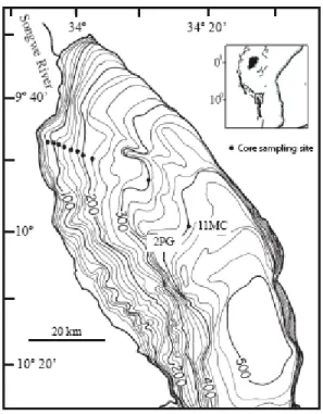
Figure 2.1. Coring locations in Lake Malawi’s northern basin, core 2MC is the most nearshore core in the sampling line (82 m water depth), and core names increase numerically until core 11MC (demarked) at 386 m water depth. Page 31.
Figure 2.2 Bulk surface sediment (0-1 cm) parameters (a) %TOC, (b) %TON, (c) C/N, (d) Si:Ti where the increase in Si:Ti from 5MC to 9MC is described by y = 0.00082x – 0.0947, R2 = 0.96, (e) δ13C in ‰, and (f) δ15N in ‰, for cores 2MC – 11MC. Error
bars (where present) represent average error between duplicate analyses. Page 32.
Figure 2.3. 10 mm averaged Si:Ti values with depth in core for cores 2MC through 9MC as obtained by XRF scanning. Page 33.
Figure 2.4. %TOC (a), %TON (b), C/N (c), Si:Ti (d), δ13C (e), and δ15N (f) with depth in
Pb-210 age-modeled cores. The five parameter values nearest the core top represent average values of analyses 0.5 cm above and below the level of age determination. Page 34.
Figure 2.5. Surface sediment (0-1 cm) percent water content by weight (filled circles) for cores 2MC – 9MC, and mean (filled triangles) and modal grain size (open triangles) for cores 4MC – 10MC, in µm. Page 35.
Figure 2.6. (a) Age vs. Depth of Pb210 dated cores 2MC, 5MC, 8MC, and 9MC (b) Calculated linear sedimentation rate; (c) calculated mass accumulation rate; and (d) calculated total organic carbon mass accumulation rate for age modeled cores 2MC, 5MC, 8MC, and 9MC. Page 36.
Figure 2.7. Diatom relative percent abundance as enumerated from surface sediment (1 cm) smear slides of cores 2MC – 9MC, divided into planktonic, tychoplanktonic, and benthic life strategy groups. Page 37.
x
Figure 3.1. Coring locations in Lake Malawi’s northern basin, core 2MC is the most nearshore core in the sampling line (82 m water depth), and core names increase numerically until core 11MC (demarked) at 386 m water depth. Page 65.
Figure 3.2. Bulk sediment parameters as measured for the 0-4 cm homogenized horizons used for subsequent fraction isolation. δ15N is reported in units of per mil (‰) as
described in the text. Page 66.
Figure 3.3. Percent relative abundance of aquatic (C20, 22, and 24) and terrestrial (C28 and 30) n-alcohols analyzed after polar lipid isolation from TLE (a), and the
concentration of each alcohol normalized to g OC of the analyzed sediment. Page 67.
Figure 3.4. Stable carbon isotopic ratio in units of per mil (‰) for bulk sediment (0-4 cm) and fractions isolated from that sediment including protokerogen, total lipid extract (TLE), and aquatic n-alcohols (C20, 22, and 24). The approximate boundary of
permanent anoxia and the potential extent of the chemocline zone are noted, although these boundaries are highly mobile and affected by numerous parameters (see text). Page 68.
Figure 3.5. Radiocarbon signatures presented as Δ14C (units of per mil, ‰) for bulk
sediment (0-4 cm) and fractions isolated from that sediment including protokerogen, total lipid extract (TLE), aquatic n-alcohols (C20, 22, and 24), and terrestrial n-alcohols (C28 and 30). The approximate boundary of permanent anoxia and the potential extent of the chemocline zone are noted, although these boundaries are highly mobile and affected by numerous parameters (see text). Page 69.
Figure 3.6. Stable carbon isotopic ratio in units of per mil (‰) of water column organic carbon fractions DIC and POC from 30 and 350 m water depth where successful. The approximate boundary of permanent anoxia and the potential extent of the chemocline zone are noted, although these boundaries are highly mobile and affected by numerous parameters (see text). Page 70.
xi
Figure 3.7. Radiocarbon signatures presented as Δ14C (units of per mil, ‰) of water
column organic carbon fractions DIC, DOC and POC from 30 and 350 m water depth where successful. The approximate boundary of permanent anoxia and the potential extent of the chemocline zone are noted, although these boundaries are highly mobile and affected by numerous parameters (see text). Page 71.
Figure 4.1. Sampling map reflecting the three sampling locations in the western arm of Lake Superior. Page 100.
Figure 4.2. Stable isotope signatures (all in units of per mil (‰)) of all organisms at all sites a) as measured without sample pre-treatment, and b) with post-analysis lipid correction applied to zooplankton species using δ13C
ex = δ13Cbulk + 6.3((C:Nbulk –
4.2)/C:Nbulk) as refined by Smyntek et al. (2007) and described in text. Horizontal error
bars represent average error in δ13C between bulk analyses with no pre-treatment and
analyses with acid pre-treatment to remove inorganics as a preparative step for radiocarbon analysis and may also represent error associated with separate instrumentation. Page 101.
Figure 4.3. δ13C versus Δ14C of surface and deep water column DOC, POC, and DIC at
all sampling locations, both in units of per mil (‰). Page 103.
Figure 4.4. Organism trophic levels from all sampling locations (a) and of multiple size classes for Mysis and Diporeia (b) as calculated by: TL(Glu/Phe) = (δ15NGlu - δ15NPhe -
3.4)/7.6 + 1 from Chikaraishi et al. 2009. Page 104.
Figure 4.5. Radiocarbon signature of organisms sampled at all locations including only large size classes of Mysis and Diporeia, in units of per mil (‰). Page 105.
1
Chapter 1: Introduction
1.1 Organic Matter in Lake Systems
Biogeochemical cycling of earth’s most biologically important elements (carbon nitrogen, oxygen, sulfur, and trace metals) is linked by the presence, transport, and transformations of organic matter. Organic matter (OM) is the material produced by living organisms and composed largely of organic compounds rich in carbon, but can also include considerable amounts of the elements listed above. Studying the chemical
composition of organic matter can provide insight to the origin of the material, the age of the material, and how that material is transported and assimilated in different
environments. In doing so, light is also shed on the functioning of major biogeochemical processes on that affect all life on earth, such as the carbon and nitrogen cycles. Almost all OM on earth originates through biologically mediated autotrophic synthesis of organic compounds from abiotic chemical sources. In lakes, organic matter produced in situ by aquatic organisms is referred to as ‘autochthonous’. This OM is synthesized from dissolved CO2 photosynthetically or chemosythetically by algae and other microbial
species. Organic matter produced by organisms outside the lake, such as
photosynthesized by land plants, is referred to as ‘allochthonous’. Organic matter can partition into different phases, including dissolved organic matter (DOM) or particulate organic matter (POM), depending on its chemical structure and the conditions of the system. DOM is operationally defined as the material passing through a 0.1 – 1.0 µm filter, while POC refers to the material retained the filter. This research utilized 0.7 µm filters for separation of water column OM fractions.
Once OM is fixed by primary producers in any system, it is either incorporated into the food chain through heterotrophic consumption or becomes part of the standing organic pool of detrital biomass of the system, where further microbial consumption often occurs. In lakes, the POM not immediately incorporated into the food web sinks out of the water column and accumulates as sediment on the lake floor. Any material not further consumed by microbial reworking after sedimentation is buried and preserved
2
long term. In this way, OM sources to lake systems can include the autochthonous material synthesized in situ, allochthonous material composed of recently fixed plant material, allochthonous material composed of aged plant and/or animal detrital material, or re-suspension of organic rich sediments which may have ultimately originated from a combination of all the above sources.
Using organic matter as a tool for learning about lake systems is typically accomplished through study of its various chemical components. Since most organic matter is composed predominately of carbon, the amount of OC is often measured to indicate the amount of organic material in a system. In lakes, the amount of OC in water column or sediment fractions is dependent on the productivity of the system and on the amount of loading from allochthonous sources. Beyond quantification of OM, natural abundance isotopic analysis of different organic matter components (such as C, N, O, S, and others) has become a powerful tool to study its origin, transport, and transformation. The C and N isotopic signatures of various OM components were used heavily in this research to learn about such processes in large lake systems.
While 12C is the vastly predominant carbon isotope in the environment (98.9%), the
stable isotope 13C constitutes roughly 1.1% of naturally occurring carbon. Stable carbon
isotope 13C can be oxidized into 13CO
2 and incorporated into organic matter through
photo or chemosynthesis. Biogenic substances typically contain greater amounts of lighter 12Cthan the substrate it was sequestered from, due to kinetic isotopic fractionation
of the isotopes; assimilation of the heavier 13C is slower and therefore selected against
(Killops and Killops, 2005; Mackenzie and Lerman, 2006). This fractionation can occur with each biological transfer of carbon, giving organic matter with distinct assimilation pathways an identifiable stable carbon signature (13C relative to 12C content, Mackenzie
and Lerman, 2006). Similar kinetic fractionations occur with respect to biochemical processes involving nitrogen. The naturally occurring nitrogen isotope 15N, which
accounts for roughly 0.4% of nitrogen atoms, is heavier than the most abundant isotope
14N (99.6%), and its slower reaction can result in products depleted in 15N. The stable
3
(δ) notation as per mil (‰) deviations from a standard according to the following equation:
δx (‰) = ((Rsample – Rstandard)/Rstandard) *1000
where R is the ratio of the heavier to lighter isotope in question and x is the element whose isotopic ratio is being measured (e.g., C or N in this research).
1.2 Radiocarbon- genesis and application as a biochemical tracer
Radiocarbon (14C) forms naturally in the upper stratosphere and lower troposphere by
neutron bombardment of 14N, which prompts the addition of a neutron and the formation
of the 14C isotope (Libby, 1946; Libby et al., 1949). This unstable isotope constitutes just
<0.0001% of all carbon atoms. Advances in analytical technology, such as the ability to isolate and analyze very small samples (Pearson et al., 1998) as well as individual
chemical compounds (Eglinton et al, 1996) for radiocarbon content are opening doors to understanding the carbon cycle in ways that were previously impossible. The ability to obtain a radiocarbon age for a substance is based on abundance of the two less common naturally occurring carbon isotopes; stable isotope 13C, and radioactive 14C relative to 12C
(Libby, 1946; Libby et al., 1949; Killops and Killops, 2005). Once formed, 14C is rapidly
oxidized to 14CO
2, allowing for incorporation into organic matter through photosynthesis
by autotrophic organisms. Upon organism death 14CO
2 accumulation ceases, at which
point the amount of 14C in an organism begins to decline, as the unstable nature of the 14C
isotope prompts its decay back into 14N (Ingalls and Pearson, 2005; Killops and Killops,
2005). Since the half life of 14C is known (5730 yr), the content of 14C in organic matter
can be compared the corresponding carbon stable isotope content to determine an ‘age’ of the material relative to modern (Killops and Killops, 2005). To isolate the age component in this measurement, the ratio of 14C relative to 12C is corrected for biogeochemical
fractionation by measuring the 13C to 12C ratio in the same sample and assuming that 14C
fractionation is twice that of 13C. This is most typically accomplished through
accelerator mass spectrometry analysis (McNichol and Aluwihare, 2007). An additional, but often useful, complication to radiocarbon measurements is the fact that above-ground
4
nuclear testing added considerable anthropogenic 14C to the global atmosphere. Therefore
‘modern’ in radiocarbon terms corresponds to the 1950s, just prior to the spike in radiocarbon from nuclear weapons testing, and it is possible for a substance to have a radiocarbon age ‘younger than modern’, expressed as ‘Fraction Modern’ values greater than 1, given the equation:
Fraction Modern (Fm) = (sample – blank)/(modern reference – blank) (McNichol and Aluwihare, 2007). Thus, organic matter with different cycling characteristics or differently aged source material can have a radiocarbon signature distinct from other material. The Fm value described above can then be used to calculate Δ14C, defined as:
Δ14C = (Fm * eλ * (1950 – yc) – 1) *1000
where Fm = the fraction modern value, λ = 1/8267, and yc = year collected, following the convention of Stuiver and Polach (1977). This transformation into Δ14C values serves
to normalize radiocarbon measurements to δ13C = -25‰ (to account for kinetic
fractionation from biological transfers), and also to correct the value to account for decay time between year of collection and year of analysis (necessary because of the declining atmospheric radiocarbon level post-1950s weapons testing).
1.3 Focusing Research on Large Lakes
Large lakes around the world are particularly useful systems from which to gain vital understanding of carbon cycling processes; however, many characteristics of the carbon cycle within these systems remain unresolved. Globally, the area covered by large lakes (those with areas greater than 500 km2) is just 0.4% of that occupied by
marine waters, however these lakes accumulate ~1/10th the amount of organic carbon
sequestered in oceanic sediments (Alin and Johnson, 2007). Despite this, the nature of carbon that accumulates in lake sediments is often unclear; for example, in Lake Malawi, one of the great African rift lakes, there are conflicting results regarding the proportion of aquatic versus terrestrial organic carbon contained in surface sediments (Filippi and Talbot, 2005; Castaneda et al., 2007). In another system, that of Lake Superior in the
5
USA (the world’s largest lake by surface area (Herndendorf, 1990)), the degree to which allochthonous carbon inputs support the aquatic food web is unclear. In this system, annual carbon balance estimates indicate that carbon export from the lake is far greater than carbon input (Cotner et al., 2004; Urban et al. 2005). Since Lake Superior has been found to be net heterotrophic in nature (Urban et al., 2005), this carbon budget imbalance suggests carbon in the lake is supplemented by an uncharacterized source, which may be allochthonous in nature, but could also be derived from old autochthonous (aquatically produced) material. These two lake systems are the focus of my research.
1.4 Lake Malawi
1.4.1 Modern Physical, Chemical, and Hydrologic Characteristics
For all their similarities, the large lakes of the world are remarkably distinct from one another in a myriad of ways, including their hydrologic regime and physical and chemical limnology. Lake Malawi, the southernmost of the Great African Rift Lakes, is no exception, exhibiting characteristics that are unique even to its northern African rift lake neighbors.
Lake Malawi is the fourth largest lake in the world by volume (7,775 km3), the
eighth largest by surface area (29,600 km2), and the third deepest non sub-glacial lake
(706 m max depth). Although it exists in an area of tropical climate, it is far enough south of the equator to experience seasonal cycling of wind, temperature, and
precipitation. A rainy season occurs from November through March, at which time the Intertropical Convergence Zone (ITCZ) lies just south of the lake. Winds during this time are predominately northerly. Around April/May the region enters a dry season when the ITCZ shifts northward, which induces a concurrent shift in wind direction to
predominately southerly (Eccles, 1974). Although the average monthly rainfall levels for Lake Malawi are actually comparable to those of the North American Great Lake
Ontario, evaporation levels on the African continent are much higher, given the more continuous warm air temperatures (Spiegel and Coulter, 1996), meaning the water budget of the lake relies heavily on evaporation to balance inputs (Eccles, 1974; Spigel and
6
Coulter, 1996). Adding to this dependence on evaporation is the nearly-closed basin morphometry; the Shire River is the lone output for Lake Malawi and is typically only a few meters in depth (Eccles, 1974). When this river was 3.5 m deep in 1974, it was estimated to account for only 20% of the water loss from Lake Malawi, with evaporation accounting for the other 80% (Eccles, 1974). A more detailed water budget calculated from compiled data by Spigel and Coulter (1996) had similar results, estimating 50 of the 52.7 km3 water/yr lost from the lake to result from evaporation (95%), with river drainage
making up the 5% difference. Lake inputs were found to be dominated by precipitation (67%), while 33% was due to river inflow and storm runoff (Spigel and Coulter, 1996). Clearly, there is a delicate hydrologic balance in Lake Malawi, in which the relative amounts of precipitation and evaporation are critically important to the character of the system.
Along with warm air temperatures, the orientation of the lake basin helps produce the extremely high evaporation rates (more than double those of Lake Ontario; Spigel and Coulter 1996) estimated in the Lake Malawi water budget. As is common in rift-formed lakes, Lake Malawi has a long, narrow shape. Although it is roughly 560km long at its longest point, it has a maximum width of merely 75km (Eccles, 1974). The north-south orientation of the lake allows the prevailing winds of the region to blow along the long axis of the lake most of the year. Relatively strong wind events with multiple day durations also occur, further facilitating high evaporation (Eccles, 1974).
These continuous and occasionally intense wind events are, however, insufficient to induce complete vertical mixing of the lake’s water column. The lake’s great depth (~700 m) and lack of significant temperature induced density fluctuations (as found in temperate great lakes; Bootsma and Hecky, 2003) prevent such mixing. The water below about 250 m therefore remains anoxic and unmixed with the oxygenated water above (Eccles, 1974; Bootsma and Hecky, 2003). This results in a meromictic mixing regime, in which the bottom ~450m of water remains isothermal (slightly less than 23°C) for the entire year and circulates internally, while the upper 250m undergoes a seasonal
7
water stratification is most pronounced during the wet season, and weakens during the dry season due to evaporative cooling and mixing induced by the dry southerly winds (Spigel and Coulter, 1996). However, the range of water temperatures between the surface and bottom waters is minimal despite the stable density gradient; water is roughly 22.5°C in the hypolimnion while a maximum temperature of roughly 29°C is reached in the epilimnion during the peak of austral summer stratification (Wuest et al., 1996). During austral winter when the surface water stratification decomposes, surface water temperatures can be as low as 23°C: a mere 0.5°C (or less) warmer than the permanently anoxic water below (Wuest et al., 1996). Complete water column mixing is prevented during these times by additional density stability formed due to chemical gradients of dissolved solids and non-ionic compounds (Wuest et al., 1996).
Although wind driven mixing is incomplete in Lake Malawi, the long lake fetch and consistent wind events allow for various water transport mechanisms to establish. Surface seiches with an amplitude of 12 cm have been observed, lasting anywhere from 6 to 24 hours (Eccles, 1974), and internal seiches are likely (Eccles 1974; Johnson, 1996). Winds traveling parallel to the long fetch of Lake Malawi can also generate longshore currents, allowing for lateral transport of sediment and nutrients along the shoreline (Johnson, 1996). Such alongshore winds can also facilitate the offshore movement of water through Eckman transport, thereby allowing for upwelling of the deeper waters (Bakun, 1990). An additional and critical water circulation process driven in part by wind is the formation of profile driven density currents. The southern basin of the lake is relatively shallow and undergoes complete mixing (Spigel and Coulter, 1996), allowing for high rates of evaporative cooling. This cooled water is more dense and subsequently sinks, where it travels along the lake’s floor following the downward sloping basin profile until it reaches the deep basin north of Nkhata Bay (Eccles, 1974). It is
hypothesized that this influx of cooled water to the anoxic bottom waters is essential in maintaining the permanent thermocline at 250m; the bottom waters must be mixing internally since they remain isothermal, therefore without an influx of cooled water sources one would expect the 250m thermocline to gradually migrate deeper as the result
8
of oscillation driven mixing with the slightly warmer water at the temperature boundary (Eccles, 1974; Johnson 1996). Wind, therefore not only affects surface water movement, but contributes to the cooling necessary to replenish the isothermal anoxic hypolimnion.
Chemically, the surface waters of Lake Malawi are relatively low in salinity and dissolved ion content (Hecky and Bootsma, 2003); while the anoxic bottom waters contain more concentrated nutrient pools. An analysis of estimated annual nitrogen, phosphorus and silicon inputs to the surface mixed layer of the lake indicate that
approximately 89% of phosphorus and 88% of silicon delivered to the mixed waters are sourced from the anoxic waters below, with atmospheric deposition and river inflow accounting for the remaining inputs (Hecky et al., 1996). Conversely, vertical transport, river influx, and atmospheric deposition combined accounted for only about 21% of nitrogen inputs to the surface waters. This deficit is balanced by very high rates of biological nitrogen fixation, particularly by cyanobacteria species (Hecky et al, 1996 and sources therein). Additionally, free hydrogen sulfide is contained in the deep anoxic bottom waters (Eccles, 1974).
1.4.2 Geologic Setting and Historic Lake Levels
Lake Malawi, along with great lakes such as Tanganyika (Africa) and Baikal (Russia), is one of only a few deep and very old lakes still in existence. Formed by an active continental rift system, it has existed for millions of years, although exact age estimates differ. It is generally believed that the Malawi Rift Basin began formation in the late Miocene, roughly ~8.6 million years ago (although earlier rifting events are also believed to have occurred), and deep water lake conditions may have existed for the past ~4.5 million years (Cohen et al., 1993; Ebinger et al., 1993; Delvaux 1995; Contreras et al., 2000). The subsequent period of nearly continuous sedimentation has resulted in over 4km of organic rich sediment accumulation in some parts of the African rift lakes (Cohen et al., 1993; Rosendahl, 1987).
This vast sediment record has been used extensively by paleoclimatologists in an effort to understand how climates, both locally and globally, have changed through time.
9
Both the world climate and Lake Malawi water levels have fluctuated historically (Johnson, 1996; Beadle, 1981). Work by Castaneda et al. (2007) (using carbon isotopes measured from plant leaf waxes within Lake Malawi sediment cores) showed that
whether or not previous wet and arid phases of southeast Africa corresponded to those of the world’s tropical regions may relate directly to the position of the ITCZ as it shifted due to glacial influence. That Lake Malawi has shown low water levels during both wet and arid phases of the continent, and that its fluctuations are typically out of phase with the Great African Lakes to the north, is likely a signal of its dependence on the position of the ITCZ (Johnson, 1996; Finney et al., 1996). By examining calcite, 14C, and diatom
records from additional sediment cores recovered from Lake Malawi, it seems the most recent major lake lowstand occurred between 6,000-10,000 years ago, when the lake was approximately 100-150m below its current level (Johnson, 1996; Ricketts and Johnson, 1996; Finney et al., 1996). Another more drastic lowstand occurred from approximately 28,000-40,000 years ago, when water levels were thought to be 200-300m below present levels (Finney et al., 1996; Johnson, 1996).
1.4.3 Primary Production and Biota
Lake Malawi is characterized by its oligotrophic nature. In a comparative study, both surface water total phosphorus (0.1 – 0.5 µmol/L) and total nitrogen (4.7 – 14.8 µmol/L) in the lake were the lowest of all measured systems, which included Lake Superior, large and small Canadian lakes, Lake Victoria, and a number of marine locations (Guildford and Hecky, 2000). These low values were attributed to a
combination of Lake Malawi’s very long mean annual flushing time of 700 years (Spigel and Coulter, 1996) and its unique deep water chemistry. Specifically, for nitrogen, a relatively high rate of denitrification occurs at the oxic/anoxic boundary of the
permanently anoxic bottom water, such that vertical diffusion of N to the surface mixed layer accounts for little to no contribution to the overall available mixed layer N (Hecky et al., 1996). Enhanced regeneration of phosphorus from metal oxides also occurs in the deep water and creates a low N:P ratio in those bottom waters. Mixing of those deep
10
waters with the water above can create limitation, which is likely balanced by N-fixation (Hecky 2000). Phytoplankton responsible for primary productivity consume nutrients in a fairly fixed proportion, and their growth is often constrained by the unique nutrient limitations of the system in question (Hecky and Kilham, 1988). Of the major required nutrients for algal growth, namely C, N, and P, both C and N are readily available from atmospheric sources and subsequent diffusion or fixation, while P does not exist in a gaseous form (Hecky and Kilham, 1988; Hecky et al., 1996). A positive correlation is often found between algal biomass, as indicated by chlorophyll a (chl a) concentration, and total P concentration in freshwater systems. This relationship is also observed in Lake Malawi and could indicate a degree of P limitation, although some correlation also exists between chl a and total N (Guildford and Hecky, 2000). As a result of nutrient dependence, primary production in Lake Malawi also seems to be highly dependent on hydrologic conditions which affect the amount of mixing that occurs between the more nutrient rich bottom waters and the surface water (Patterson et al, 2000). Some of the earliest studies of primary production rates in Lake Malawi observed that maximum production and plankton biomass occurred during the surface water mixing period of May to September (Degnbol and Mapila, 1982). This trend was generally supported by a two year investigation of light attenuation and production in Lake Malawi’s central basin, which found average annual primary production to be 329.4 g C m-2y-1 for 1992, and 518.3 g C m-2yr-1 for 1993, and concluded that the greater
production in 1993 was a result of increased seiche activity in that year and increased mixing (Patterson et al., 2000). Other estimates of primary production in Lake Malawi are nearer to 240 g C m-2 yr-1 (Guildford and Hecky, 2000).
Phytoplankton of Lake Malawi are dominated by Cyanophyta (cyanobacteria), Chlorophyta (green algae), and Bacillariophtya (diatom) species (Lehman, 1996). The open-water zooplankton community is relatively species poor, and is dominated by just four crustacean species; a calanoid copepod (Tropodiaptomus cunningtoni), two
cyclopoid copepods (Mesocyclops aequatorialisaequatorialis and Thermocyclops neglecus), and a cladoceran (Diaphanasoma excisum) (Lehman, 1996; Irvine and Waya,
11
1999). Most pelagic zooplankton are preyed upon by the lakefly Chaoborus edulis and larvae of the cyprinid fish Engaulicypris sardella, though numerous other pelagic fish species exist that also feed to a lesser extent on the open water zooplankton population (Lehman, 1996; Irvine and Waya, 1999). In general, the fish community of the lake is dominated by the remarkably diverse community of cichlid species. This group of fishes is thought to have existed in Lake Malawi for roughly 700,000 years, and over 400 species of cichlids are endemic to Lake Malawi alone (Moran et al., 1994). This
remarkable speciation has been a point of extensive study for evolutionary and molecular biologists, and it is believed that species radiation occurred quite rapidly in the lake via three bursts of cladogenesis, and may actually be monophyletic in origin (Moran et al., 1994; Albertson et al., 1999; Danley and Kocher, 2001). This rapid species radiation has resulted in extremely specified feeding strategies that include piscivores, planktivores, lepidophages (scale eaters), fin biters, ectoparasite cleaners, molluscivores, crevice feeders, periphyton feeders, aufwuchs feeders (algae growing on surfaces other than plants), and paedophages (those that steal eggs or larvae from mouth-brooding cichlid species) (Albertson et al., 2003).
1.5 Lake Superior
1.5.1 Physical, Chemical, and Hydrologic Characteristics
Lake Superior differs substantially from Lake Malawi in a number of ways, but not in its large size. Lake Superior is the largest lake in the world by surface area (82,100 km2) and the third largest by water volume (12,200 km3), though, with a maximum depth
of ~400m, it is much shallower than Lake Malawi. It is located in an area of temperate climate in North America, and experiences four distinct seasons that each differ in temperature and precipitation patterns. The combination of this climatic seasonality and the relatively shallow depth of Lake Superior creates a dimictic mixing cycle within the lake, whereby the entire water column mixes completely twice a year, in spring and fall, and reaches stratification in both summer and winter between mixings (Bennet, 1978). The lake experiences at least partial ice cover each winter, and the freezing or near 0°C
12
surface water allows for the formation of a relatively weak inverse winter stratification, since the temperature of maximum water density is 4°. The relatively brief period of warming combined with the lakes large volume results in the coldest average surface water temperatures of all the Laurentian Great Lakes, with average summer and winter temperatures only 12 - 16°C and 0 - 2°C, respectively (Bennet, 1978). Recent evidence from Austin and Colman (2007) indicates that the surface water of Lake Superior is warming more rapidly than the associated increase in atmospheric temperature, and average summer surface water seems to have warmed by ~2.5°C over the traditional averages in the last three decades. This exaggerated warming was attributed to an approximately 11% reduction in winter ice over the last century, and has likely
influenced the mixing dynamics of the lake, apparently extending the average length of the summer stratification by ~25 days (Austin and Colman, 2008). Additionally, the strength and persistence of wind events over the lake may be increasing as a result of the reduced water-air temperature gradients (Desai et al., 2009). This has implications for change to major circulation and vertical mixing events, as most are predominantly wind driven (Desai et al., 2009 and sources therein).
Lake Superior’s water budget is much more hydrologically balanced than that of Lake Malawi. River output counts for 59.7% of major water losses and evaporation makes up the remaining loss (40.3%), while river input (with runoff included) and precipitation account for 43.5% and 56.5% of water contribution, respectively (Spigel and Coulter, 1996; Bootsma and Hecky, 2003). This illustrates a system much less reliant on evaporative loss and more equally influenced by major water inputs and outputs.
In Bootsma and Hecky’s comparative study of African and North American great lakes (2003), Lake Superior had the lowest conductivity and dissolved ion concentration of the eight lakes in question. Though Lake Superior’s flushing time of roughly 170 yrs is much longer than other Laurentian great lakes, it is much shorter than that of Lake Malawi (~700 yrs). The extremely low ion concentrations and conductivity despite its relatively long flushing time illustrates the unreactive nature of the granitic bedrock in
13
which the lake sits, which contributes little in the way of dissolved nutrients to the lake (Bootsma and Hecky, 2003). The dissolved silica content within Lake Superior is 38 times greater than that of Lake Ontario, and 4 times greater than that of Lake Michigan, though less than 0.001% of oceanic concentrations (Schelske, 1985). Concentrations of major metal ions are generally considered uniform across most of the lake, with slightly more variation seen in the far western arm adjacent to the city of Duluth, MN, though seasonality of nitrates and silica are observed in the surface layer as a result of annual production cycles (Weiler, 1978).
1.5.2 Geologic Setting and Historic Lake Levels
The Lake Superior basin exists almost entirely in the Canadian Shield, a large area of exposed Precambrian metamorphic and igneous rock which is highly resistant to weathering (Matheson and Munawar, 1978). Basin shaping was the result of multiple glacial erosion events, and lake formation began ~11,000 years ago as a result of both isostatic rebounding and ice shelf retreat, reaching deep water levels around 10,000 years ago. The major Sault Ste. Marie outlet formed roughly 2000 years ago, establishing the lake in its present form. Sediment underlying Lake Superior is 20-40m deep, and consists of a 10-30 m base of glacial till overlain by roughly 10 m or less of recently deposited material. Linear sedimentation within the lake is low, 0.1 – 2.0 mm/yr, and consists of relatively low organic content material rich in iron oxides (Matheson and Munawar, 1978). Since the initial fluctuations caused by isostatic rebound and melting ice shelves as the lake formed, lake levels have remained relatively constant since the occurrence of deep-water conditions.
1.5.3 Primary Production and Biota
Lake Superior is also classified as an oligotrophic lake. Nutrient structure of lake water is unique due to its relatively high surface water total nitrogen (20.4 – 31.9 µmol/L) and low total phosphorus (0.1 – 0.3 µmol/L) (Guildford and Hecky, 2000). This extreme stoichiometric imbalance has been a focus area of study, and it seems the discrepancy is
14
becoming further exacerbated as nitrate (NO3-, which accounts for ~80% of total water
N) seems to have been increasing in concentration since the 1980’s (Sterner et al., 2007). Early explanations for this NO3- buildup included the conclusion that much of the NO3
-was sourced from atmospheric deposition to the lake (Ostrom et al., 1998). In contrast, by examining whole lake NO3-and total N budgets in conjunction with stable oxygen
isotope analysis of NO3- and potential nitrate sources, Sterner et al. (2007) concluded that
substantial amounts of the NO3- within the lake must originate from in-lake oxidation of
reduced N forms. They suggested a number of mechanisms in support of their conclusion: a greater contribution from ammonia oxidizing microbes than previously recognized, recognizing that the biotic consumption of NO3- is generally constrained by
the lack of phosphate availability, and inferring that denitrification may be limited since organic C within Lake Superior is not sufficient to induce the anoxic conditions (which can result from oxygen consumption during organic carbon decay) appropriate for high levels of denitrification (Sterner et al., 2007). Primary production in this unique nutrient system is extremely low in comparison to other great lakes of the world, just 65 g C m-2
yr-1, compared to 100 – 170 g C m-2 yr-1 in other Laurentian Great Lakes and 240, 290,
and 1500 g C m-2 yr-1 in African lakes Malawi, Tanganyika, and Victoria (Hecky, 2000).
In an extensive study of primary production in Lake Superior, lowest rates typically occurred at open lake sites, while the highest rates were measured at select nearshore locations (Munawar et al. 2009).
Unsurprisingly, the increase in water temperature of this temperate lake
associated with the warming season between May and September also corresponds to an increase in phytoplankton biomass from about 70 to 150 mg/m3 for that same time period
(Munawar and Munawar, 1978). More recent research has reported much higher phytoplankton biomass, though a smaller relative increase from 948 to 1069 mg/m3
between spring and late summer seasons (Munawar et al., 2009). Generally,
phytoplankton in Lake Superior are dominated by phytoflagellates (53%) and diatoms (38%), with cyanobacteria and green algae making up the difference (Munawar and Munawar, 1978). Munawar et al. (2009) observed that diatom biomass increased by
15
~70% in the lake between spring and summer, while biomass of Cyanophyta decreased by 60%. This also resulted in an increase in average plankton cell size between the seasons, though spatial variability was high (Munawar et al., 2009). Lake Superior also supports a large and diverse community of picoplankton, organisms <0.3 µm, which are responsible for up to 50% of total primary production (Fahnenstiel et al., 1986). This group consists of eukaryotic flagellates, non-motile eukaryotic cells, and chroococcoid cyanobacteria including new species of Synechococcus spp. not described elsewhere (Fahnenstiel et al., 1986; Ivanikova et al., 2007). The zooplankton community is dominated by crustacean species, and biomass is often predominantly composed of copepods such as Limnocalanus macrurus, Diaptomus sicilis, and Diacyclops thompsoni,
the three of which have been shown to make up 99% of the crustacean zooplankton biomass in May (Brown and Branstrator, 2004). Other important zooplankton species include cladocerans such as Daphnia mendote, Bosmina longirostrus, and Holopedium gibberum, as well as the predators Mysis relicta and invasive Bythotrephes longimanus,
and the benthic amphipods Diporeia spp. Fish species in the lake’s offshore zone are characterized by deepwater scuplin (Myoxocephalus thompsonii), siscowet lake trout (Salvelinus namaycush siscowet), and the Coregonids kiyi (Coregonus Kiyi) and lake herring (Coregonus artedi). Nearshore fish communities are similar though include many more species in lower abundance, most notably rainbow smelt, wild lake trout, lake whitefish, longnose suckers, and sticklebacks (Gamble et al., 2011b). Despite the greater species diversity nearshore than offshore, both communities were found to have similar food web structures that are primarily supported by Mysis and Diporeia (Gamble et al. 2011b).
1.6 Objectives of this dissertation
The goal of this research was to carry out a comprehensive and systematic study of how organic matter cycles between, and within, different parts of large lake systems, and the results of that work are described in this dissertation. Research was approached in two parts; first, by focusing on organic matter that is deposited as lake sediments in
16
Lake Malawi, Africa. First, parameters traditionally used to characterize sediment organic matter and mineral composition were examined across a nearshore to offshore transect, to determine if proximity to shore was reflected by these values. Characteristics of sediment such as %TOC, %TON, δ13C, δ15N, Si:Ti, and diatom microfossil
abundances were examined, and this work is described in chapter 2. Then, focus was placed on the organic carbon component of the same sediment transect in Lake Malawi, by using compound class specific radiocarbon dating in combination with stable isotope signatures to tease apart the sources and ages of this sediment-sequestered carbon. That work is presented in chapter 3. Research focus then shifted to the food web of Lake Superior, USA, to investigate how organic matter is transferred between trophic levels and major organisms. Compound specific stable nitrogen isotope (CSNIA) of amino acids was applied to characterize trophic position of major food web organisms, and radiocarbon signature of major zooplankton and fish species was applied to shed light on the age of carbon sources to the food chain. This work constitutes chapter 4 of this dissertation. Together, these studies provided a thorough and novel understanding of how carbon inputs are utilized, cycled, and preserved within large lakes.
17
Chapter 2: Characterizing sediment compositional change with water depth and distance from shore in a tropical rift lake
This chapter examines traditionally applied methods of paleolimnology to determine if sedimentary parameter response can in fact indicate proximity to lakeshore in a modern great lake system. Almost all parameters were found to reflect changing distance from shore and water depth in a manner consistent with their traditional
interpretations in sediment records, which are often used to infer previous lake level and regional climate conditions. With increasing water depth and distance from shore, generally, grain size decreased while sediment water content increased, %TOC increased, and both δ13C and C/N decreased, although each record records subtleties reflecting
terrestrial input nearshore and changing water chemistry as distance from shore increased. Si:Ti also increased concurrently, and chemocline position was clearly reflected in the sedimentary record. Diatom microfossil abundance showed a shift from tychoplankton domination nearshore to planktonic species domination offshore, while benthic species contribution remained consistently low throughout.
2.1 Introduction
Discerning the history of hydroclimate in a lake catchment is a major goal of paleolimnology, and one way this is accomplished is by estimating historic changes in lake level. Environmental changes that influence local hydrology and lake level also induce considerable change in sediment composition, due to the heavy influence hydrologic balance has on lake water chemistry, ecosystem composition, and sedimentation processes (Scholz, 2002). This may lead to changes in sediment
composition with water depth and distance from shore, for example in grain size, fossil assemblages, abundance and composition of organic and inorganic constituents (Gasse and Street, 1978; Hofmann, 1998; Winder and Schindler, 2004). These and other parameters preserved in the sediment record, such as C/N ratios in bulk organic matter, may therefore indicate historic proximity to lakeshore and influence from terrestrial
18
sediment sources, and subsequently past lake level and hydroclimate (Fritz, 1996; Alin and Cohen, 2003; Scholz et al, 2007).
In Lake Malawi, the southernmost of the East African great lakes, sandy
horizons in some deep-water sediment cores have been interpreted as nearshore deposits, indicating past times of lower lake level (Finney and Johnson, 1991). Relative
abundances of planktonic versus benthic diatom species in fossil assemblages have been used to infer lake level changes in Lake Malawi and other great lakes, and are a viable proxy due to the sensitivity diatom species exhibit to their aquatic environment (Owen and Crossley, 1992; Wolin et al., 2001; Gasse et al. 2002). The C/N ratio, in concert with carbon and nitrogen stable isotope composition of bulk organic matter in Lake Malawi sediment cores, has been interpreted to reflect aquatic versus terrestrial dominance of organic matter, and as an indication of proximity to shore and terrestrial inputs (Fillipi and Talbot, 2005).
While these indicators are widely applied, little examination of these parameters has occurred in the modern sediment of tropical rift lake basins to assess their actual sensitivity to water depth or proximity to lakeshore. The goal of this study was to determine which of these, and other, commonly applied sediment proxies may in fact vary systematically with distance from shore. We analyzed ten short cores from the northern basin of Lake Malawi, recovered along a depth transect from a major river mouth and extending into the lake’s deep offshore basin. Developing a relationship between modern water depth (and therefore distance from shore) and sediment chemical signature serves as a test of past interpretations of historic lake levels from long sediment cores that were based on some of the parameters described above.
2.2 Methods
2.2.1 Sediment Collection
Ten short cores (M09-2MC to M09-11MC) were recovered with an Ocean Instruments Multi-Corer from the northern basin of Lake Malawi in 2009 aboard the Malawi Fisheries vessel F/V Ndunduma. The core sites were located on the prodelta
19
slope of the Songwe River, beginning approximately 7.8 km from the river mouth in 81.7 m depth and extending down into the lake’s deep offshore basin to a depth of 386 m (Fig. 2.2.1). The core transect line was surveyed with a swept frequency pulse (CHIRP)
seismic reflection profiling system (Fig. 2.2), and care was taken to avoid coring in slumped or disturbed areas. Upon recovery of the multi-corer, the top 3 cm of one of the four cores with a well-preserved sediment-water interface was extruded in 1cm intervals. Extruded horizons were placed in glass jars with Teflon-lined lids, and immediately frozen. The remainder of this core and a second whole core were capped and stored in a refrigerator at ~4º C prior to shipment back to the U.S. Cores and frozen samples were air-freighted back to the Large Lakes Observatory (LLO), for subsequent stratigraphic and sedimentological analyses.
2.2.2 Sediment Analyses
The completely intact core from each site was scanned for magnetic susceptibility and bulk density with a Geotek standard multi-sensor core logger at the LacCore facility at the University of Minnesota Twin Cities Campus. Each core was then split lengthwise into working and archive halves. The archive half was first digitally imaged with a DMT CoreScan Digital line scan camera and subsequently transported to LLO and scanned at 1 mm resolutionfor elemental analysis on an ITRAX X-ray Fluorescence Core Scanner (Cox Analytical Systems,60 sec scan times using a Mo x-ray source set to 30 kVand 15
mA). The working core-half was sampled at LRC every 10 cm in core 2MC and every 5 cm in cores 3MC through 9MC for inorganic and organic elemental and isotopic
analyses. Approximately 3-4 ml of wet sediment were extracted with a modified syringe and transferred to pre-weighed 5 ml vials for elemental and isotopic analysis.
Additionally, smear slides were prepared at 3cm intervals from cores 2MC-9MC for microscopic analyses and 20-30 mg of surface sediment was collected for grain size analysis. Cores 2MC, 5MC, 8MC, and 9MC were subsampled for 210Pb dating analysis.
Core subsamples were weighed pre- and post-freeze drying to determine water content. Total carbon and inorganic carbon were determined using a UIC Carbon
20
Coulometer calibrated to pure calcium carbonate. Duplicates were run every sixth sample and standards every ten samples. Total carbon measurements were obtained by six minutes of combustion at 950˚C, inorganic carbon content was determined by exposing a second aliquot of the same sample to 2N HCl for six minutes. A Costech Elemental Analyzer coupled to a Finnigan Delta Plus XP Mass Spectrometer was used to determine total organic carbon, total organic nitrogen, 13C (+/- 0.42‰, accurate within
0.97%), and δ15N (+/- 0.15‰, accurate within 5.6%) of bulk sediment after acid
fumigation to remove carbonates. Briefly, after sediment was weighed into tin capsules, 10 uL of milli-Q water was added to each, and the samples were left in an enclosed dessication chamber with an open beaker of 12N HCl for 8 hours. Samples were then left on a 40°C hot plate covered lightly in foil for 8 hours to allow acid fumes to dissipate, then dried in a 60°C oven.
Relative abundances of diatom genera were determined by petrographic microscope examination of smear slides at a magnification of 200X. Quantification focused on common genera including Stephanodiscus, Aulacoseira, Surirella, Navicula
and Fragilaria as well as diatom fragments. A minimum of 300 individuals or fragments were enumerated per slide for relative percent abundance calculation.
Grain size analysis of bulk surface sediments was conducted on a Beckman Coulter LS 13 320 Laser Diffraction Particle Size Analyzer after removal of carbonates,
organic carbon, and biogenic silica. Inorganic carbon was removed by treating the sample with 6M HCl for 2 hours in a 70˚C water bath. Samples were subsequently rinsed in deionized water and centrifuged at 2800 RPM three times for HCl removal. Organic matter was removed by addition of 10% H2O2 and immersion in a 70˚C water bath for
two days, followed by three rinses as described above. Biogenic silica was removed by subjecting the sample to 0.5M NaOH for 45 min at 85˚C. These samples were rinsed 4x in de-ionized water (as above) to ensure no residual NaOH remained to interact with inorganic sediment components. The prepared samples were then introduced to the grain size analyzer.
21 2.3 Results and Discussion
2.3.1 Si:Ti
The ratio of Si to Ti (each determined by XRF scanning) in 0-1 cm surface sediment is relatively stable at 0.05-0.06 in the first three near-shore cores (2MC-4MC), followed by a sharp drop to 0.02 in core 5MC and a steady linear increase (R2 = 0.96) to
0.09 in core 9MC (Fig. 2.2d). The normalization of sedimentary silica content to that of titanium helps remove dilution effects, since titanium exists mainly within detrital mineral matrices and is therefore little affected by digenesis (Brown et al., 2000). Furthermore, the XRF measured Si:Ti ratio in Lake Malawi has been shown to correlate linearly to the biogenic silica (BSi) content of sediment as: %BSi = 142.86(Si:Ti) – 7.14 (Johnson et al., 2011). Therefore, the observed trend in surface sediment Si:Ti with water depth in Lake Malawi is a reflection of BSi content and preservation in the system.
The discrepancy in Si:Ti values between the first three cores and the following occurs at a depth where influence from the chemocline likely occurs. While the
chemocline is typically believed to exist between ~170-200 m, chemocline boundaries are not static and the zone of altered water chemistry (including fluctuations between oxic and anoxic states) could reach 141 m where core 5MC was collected (Halfman, 1993; Vollmer et al., 2002). Water column profiling done in January of 2010 by Woltering et al. (in prep) showed the suboxic zone to extend to roughly 140 m water depth. However, the observed shift in Si:Ti is more likely a result of shifting Si source than an altered chemical condition of the water column. Although other researchers have proposed an increase in BSi preservation in anoxic bottom water due to a saturation of soluble reactive Si which discourages BSi dissolution (Bootsma et al., 2003), the inverse relationship between Si:Ti and sediment grain size across the sampling line (Fig. 2.2d) suggests the relative contribution of inorganic Si is shifting as distance from shore increases. Grain size has been found to correlate positively with quartz content in large lakes (Thomas, 1969), a mineral composed of SiO2. Therefore, the sharp drop in Si:Ti
ratio at the 145m water depth is likely a reflection of decreasing quartz (and therefore silica) content of the sediments as distance from shore increases and larger grains settle
22
out of solution. The subsequently increasing Si:Ti ratio as water depth increases likely reflects the greater relative influence of BSi production on sediment silica content at more open lake sites.
Some downcore vertical structure is apparent for Si:Ti, namely in cores 4MC and 6-8MC, which show generally increasing Si:Ti with core depth. Considering downcore Si:Ti values between coring sites, there is a general trend of lower values found in the most nearshore cores, increasing with water depth and distance from shore (Fig. 2.3). Core 5MC is an obvious outlier to this trend, with the depressed values seen in this core’s surface sediment propagated downcore. There is no evidence to suggest this core is disturbed or is influenced by turbidites, as indicated by 210Pb data (discussed below).
Over much longer geologic timescales than is represented by these cores, periods of increased Si:Ti in Lake Malawi’s northern basin sedimentary record are interpreted either as periods of increased riverine transport of dissolved silica to the lake, low lake level (if fossilized periphytic diatom abundance is also high, indicating a shift in habitable benthic surface area), or a period of predominant or strong northerly winds in the region
promoting upwelling, production, and subsequent diatom burial in the north basin (Johnson et al, 2011, Brown et al, 2007, Johnson et al., 2002). Given the results presented here from a nearshore to offshore examination of surface sediment Si:Ti, it becomes apparent that consideration for the relative contribution of mineral silica sources versus biogenic sources must be included in paleoclimate interpretation of Si:Ti records. Though, again, a large shift in Si:Ti sedimentary record may be attributed to shifting chemocline position affecting the silica dissolution rate. A shifting chemocline would also affect sedimentary preservation of metal species, as a changing redox state affects dissolution and precipitation of numerous metal species. Brown et al. (2000) used downcore concentrations of multiple metal species to infer past lake conditions and resulting chemocline shifts in a core from Lake Malawi’s central basin. Of the cores in this study that exhibit downcore trends in Si:Ti, there were no apparent concurrent downcore trends in Fe, Mn, or Al concentration (as analyzed by XRF, data not shown here), indicating that there was no significant shift in chemocline across the timeframe
23
represented by these cores. This also supports the previous conclusion that the large variation in Si:Ti seen in nearshore to offshore surface sediment is reflective of shifting contribution from different silica source pools.
2.3.2 Elemental and Isotopic Analysis
Elemental composition and isotopic signatures of sediment in this study are consistent with other reported values for the northern basin of Lake Malawi (Filipi and Talbot, 2005; etc etc). Surface sediment (0-1 cm) percent total organic carbon (TOC) increased from ~2% in nearshore cores to values of 3-4% in the most off-shore cores, while total organic nitrogen (TON) content also increased steadily from ~0.2% in nearshore cores to ~0.4% in the most offshore cores (Fig. 2.2a,b). The decrease in %TOC in the most nearshore cores likely reflects dilution by clastic material from river inflow. TOC content often increases as grain size decreases in aquatic systems as a result of differing sediment density, porosity, and adsorption ability between grain sizes
(Thompson and Eglinton, 1978; Burdige, 2007), a trend that is confirmed here with comparison to the surface sediment grain size record of these cores (Fig. 2.5).
Resulting surface sediment C/N ratios (by weight) decreased from roughly 10 in nearshore cores to 8.3 in the deepest offshore core (Fig. 2.2c). C/N ratio is a common parameter used in the interpretation of both modern and paleo sedimentary organic matter source, with fresh phytoplanktonic OM having C/N values of 4-10, while that of vascular plants is often over 20 (Meyers and Teranes, 2002). It has been shown, however, that primary producers in highly N-limited systems can produce OM with significantly higher C/N (Healy and Hendzel, 1980). This is noteworthy, as Lake Malawi has been shown to experience both N and P limitation (Guildford et al., 2003). Subsequently, Hecky (1993) has proposed that in Lake Victoria phytoplankton produce OM with C/N <8.3 without N limitation, 8.3-14.6 under moderate N limitation, and can achieve values >14.6 under severe physiological N-limitation. However, C/N values of sedimentary OM resulting from each N-limitation situation are likely slightly higher, as sedimentation and diagenesis tend to selectively consume N within the first few centimeters of sediment,
24
beyond which C/N values stabilize. Talbot and Laerdal (2000) suggest that sedimentary C/N increases by roughly 5 units within the first three centimeters of Lake Victoria surface sediment. To account for the likelihood that OM was produced under N-limiting conditions in that lake, they added 5 to the ranges proposed by Hecky (1993) to allow for interpretation of OM source using downcore C/N values that had been altered by
diagenesis. The 0-1 cm surface sediment C/N values reported in this study (Fig. 2.2c) are well within the range of predominant photosynthetic production, and in comparison to the limitation scenarios proposed for Lake Victoria, fall within the range of no
N-limitation assuming some effects of diagenesis, or moderate N-N-limitation assuming little effects of diagenesis. Recently obtained biomarker abundance values from sinking particulates collected from sediment traps in Lake Malawi show that biomarkers of N-fixing cyanobacteria (heterocystous glycolipids) vary seasonally in abundance. This indicates seasonal variation in nitrogen limitation, as cyanobacteria are most abundant when there is some degree of N-limitation (Werne, J., University of Pittsburgh, personal communication).
Surface sediment δ13C decreased from about -22‰ nearshore to -24.9‰ offshore
(Fig. 2.2e), while δ15N is enriched in nearshore cores, around 2.7‰, decreasing rapidly at
4MC, and continuing to decline to about 0.5‰ in the most offshore cores (Fig. 2.2f). While these δ13C values overlap with the range typically associated with C3 land plants
(C3 plants: δ13C -25 to -35, C4 plants: δ13C -10 to -16), the very low corresponding C/N
values indicate a prominent lacustrine algae source at all sampling locations (Meyers, 1997). The slightly heavier δ13C values nearshore may reflect limited influence of
carbon sourced from maize, a C4 agricultural crop that has increased in cultivation within the Lake Malawi watershed in recent decades (Orr, 2000; Heck et al. 2003). While C/N values in this range could also reflect contribution from soil or sediment microbial sources (Peterson and Fry 1987; Fry 1991), the increasing BSi through this transect (as described above) supports the interpretation of diatom predominance, particularly as water depth increases. Therefore, the depletion of δ13C and decreasing C/N in