Storage characterization through gravity-meter experiments and stream flow analysis: Consequences for dry weather flow prediction

(1)

Storage characterization through gravity-meter

experiments and stream flow analysis:

Consequences for dry weather flow prediction

Chillara ReddyVaraprasad

A Thesis Submitted to

Indian Institute of Technology Hyderabad In Partial Fulfillment of the Requirements for

(2)

Department of Civil Engineering

(3)

Declaration

I declare that this written submission represents my ideas in my own words, and where ideas or words of others have been included, I have adequately cited and referenced the original sources. I also declare that I have adhered to all principles of academic honesty and integrity and have not misrepresented or fabricated or falsified any idea/data/fact/source in my submission. I understand that any violation of the above will be a cause for disciplinary action by the Institute and can also evoke penal action from the sources that have thus not been properly cited, or from whom proper permission has not been taken when needed.

————————– (Signature) ————————— ( Chillara ReddyVaraprasad ) —————————– (Roll No.)

(4)

Approval Sheet

This Thesis entitled Storage characterization through gravity-meter experiments and stream flow analysis: Consequences for dry weather flow prediction by Chillara ReddyVaraprasad is approved for the degree of Master of Technology from IIT Hyderabad

————————– (Dr. Chinthapenta R Viswanath) Examiner Dept. of Mech and Aero Eng IITH

————————– (Dr.Basudev Biswal) Adviser Dept. of Civil Eng IITH

————————– (Dr. KBVN Phanindra) Co-Adviser Dept. of Civil Eng IITH

(5)

Acknowledgements

This dissertation would not have been possible without the guidance and help of several individuals who in one way or another have contributed and extended their valuable assistance in the preparation and completion of this study. First and foremost, I would like to convey my sincerest gratitude to Dr. Basudev Biswal for his guidance and supervision throughout the tenure of this project. It was his encouragement, co-operation and support that led to the successful completion of this dissertation.

I am sincerely indebted to research scholar Swagat Patnaik for providing discharge data set , helping me in learning Q-GIS and also for helping me in carrying the experiments.

I extend my gratitude to all my friends especially Anitha Nag, Durga Sharma, Ankith Deshmukh, Shashi Ranjan and Lokesh Kumar for their kind and timely co-operation in all aspects for the completion of this dissertation. Last but not the least, I would like to owe my deepest gratitude to my parents and family members whose love and blessings have been a constant source of motivation and strength.

(6)

Dedication

(7)

Abstract

Dry weather flow prediction is important as streamflow during dry or rain-less periods, i.e. water available for various usages, is generally very low. Generally hydrological models are employed to predict dry weather flow. However, they keep several parameters whose values need to be determined through calibration, which is a cumbersome process. Furthermore, models usually under perform during low flow periods. The main aim of this study is to predict low flow by utilizing as much less information as possible. We achieve this by exploiting the recent finding that dry weather

flow characteristics are influenced by past discharge. In particular, the recession coefficient k (in

−dQ/dt =kQα_{) displays a power law relationship with past average discharge:} _k _∝_Q−λ

N , where

QN is the average discharge during pastN to 2 days before the recession event. The strength of the

relationship can be measured in terms of coefficient of determination (R2

N), and a higherR2N implies

that we can have prediction ofkfromQN. GenerallyR2N decreases withN, although for some basins

the opposite can happen, which indicating that there exists an optimal way of obtainingkfrom past

discharge. In this study, we propose a novel algorithm that gives better performance of kin most

of the cases. The consequence is that low flow discharge observed during dry weather periods can be predicted by integrating the power law equation for discharge, which can be achieved in several ways, each of them making a distinct approximation that requires different input information. Each

of the method is evaluated by considering multiple indicators such as R2 _{and NSE and PBIAS}

(percent bias). The performances are generally falling within acceptable ranges mentioned in the hydrologic literature. We also found that performances of the models can be explained by catchment characteristics. In summary, our study opens a new avenue of predicting low flow discharge by just considering past discharge.

In this study we also employed an experimental setup for observing the gravity variation at microscale for the purpose of detecting the effect of storage fluctuations on variability of gravity. For this we observed the gravity values at 12 stations in a roughly straight path at IIT Hyderabad in ODF campus. We noted down the weekly gravity values for a period of three months (August 2015 to December 2015). After applying the suitable corrections for various factors like latitude, elevation it was observed that the storage fluctuations has considerable effect on the variability of gravity values at micro scale. Our study proves that gravity variability at micro scale can be employed for hydrological modelling.

(8)

Introduction

During the dry weather period, very little water will be available for various purposes like domestic water supply (see figure 1.1), hydro electric power generation, minimum flow to treat the discharged pollutants [1, 2, 3]. Unfortunately less number of successful attempts were made in the study of low prediction models compared to the flood forecasting models. So there is a huge need to focus on low flow forecasting, as a consequence predicted low flows will be very useful for effective water quality and quantity management. A number of rainfall runoff models like HBV, IHACRES are frequently used to predict daily stream flow with a considerable accuracy. These models are complex and are data demanding [4], so streamflow prediction with limited data is always a basic challenging task in the field of hydrology. Razavi et al. [4] gave an exhaustive review on the existing low flow prediction models and also about their necessary input data, validity and limitations.

(15)

Figure 1.1: The picture depicts the water crisis in India especially during summer. The Latur water train with 50 wagons (Each wagon with one lakh liters) brings water from Sangli which is

342 km away from Latur. (for full details see http: //indianexpress.com/article/india/

(16)

The gradual diminution of discharge due to the evapotranspiration, interception (Which accounts 95% of precipitation in arid regions), during the low precipitation or no precipitation periods is termed as the recession flow. Analysis of recession flow provides significant information of storage characteristics of basin as it is mainly constitutes the subsurface flow and this can be done by ascertaining the patterns in the recession events and by connecting with the physical properties of the basin with the help of analytical models [5, 6, 7, 8, 9].

1.1 Objectives of the Thesis

The main objective of the research is to propose a novel algorithm for the better prediction ofkthat

can be further used for the prediction of dry weather flow. The sub-objectives includes

1. Investigating the variability of recession constants (α,k) across each recession event

2. Identifying the dominant factors for the prediction of recession coefficientk from the literature

3. Studying the anomaly of relationship of recession coefficientk with past discharge for the

Cali-fornia basins and investigating the reasons causing the anomaly

4. Proposing a novel algorithm for the improved prediction of recession coefficientk

5. Predicting the dry weather flow with the help of improved recession coefficientk

6. Evaluating the model performance for various prediction methods

7. Observing the spatial and temporal variation of relative gravity and investigating whether the micro study of gravity variation can be used for hydrologic study or not.

1.2 Organization of Thesis

This Thesis is organized as six chapters. The brief description of each chapter is given below. Chapter 1 deals with the motivation of research with brief description of study area along with the main and sub-objectives of research were discussed at the end.

Chapter 2 deals with comprehensive literature on some of the existing works in the field of hy-drology with emphasis on behavior of recession parameters and their prediction. Various model evaluation parameters that has undertaken in this study along with their reportable values were

(17)

also included in this chapter. Various factors affecting the relative gravity and their corrections was discussed at the end.

Study area and data used in this study was discussed in 3.

Chapter 4 deals with the novel approach for the better prediction of kcompared to the existing

literature and consequently dry weather flow by taking one basin as an example. It also includes the procedure involved in observing the relative gravity at the end.

Simulation results, the efficiency of model along with detailed figures and Corrected values of relative gravity and the factors causing variability were discussed in chapter 5.

Summary , limitations of work and the future scope of work was presented in chapter 6. Code and the supplementary material was provided in chapter 7

(18)

Chapter 2

Literature review

2.1 Storage-Discharge relationship

Generally recession flow can be expressed as a function of time variable tas Q=Q(t), whereQis

the rate of flow at the outlet of the basin at timet. Most of the recession studies suffers from the fact

that, there is no theory that gives the exact starting of recession flow. However it was eliminated by

Brutsaert (1977), who expressed discharge rate (dQ_dt) as a function of discharge (Q) as given below .

−dQ

dt =kQ

α _(2.1)

where α and k are the constants which depends on the recession characteristics. dQ_dt and Q are

computed as −dQ_dt = (Qt+∆t−Qt)

2 and Q=

(Qt+Qt+∆t)

2 [5]. The above mentioned equation can be

derived from Boussinesq’s work who proposed a nonlinear differential equation governing unsteady flow from an unconfined aquifer to a stream channel which is valid under ideal conditions of no inflow and outflow like leakage, recharge, evapotranspiration. Hence the adaptation of the above expression may not yield good results if the basin has human abstractions like storage structures, dominant evapotranspiration losses, and involvement of overland flow, diversion head works [11, 6, 12, 13, 14].

(19)

2.2 Variability of recession constants (

k

and

α

)

Due to the high variation in the sub sequent segments of recession curve, αandk are expected to

vary in the individual recession events. But Biswal and Kumar (2014) revealed that αis almost

invariant across each recession event whereas kis highly variant and this emphasizes the dynamic

behavior of storage-discharge relationship (−dQ_dt =kQα_).

Biswal and Kumar (2014) calculated αof each recession event and median of distribution

(cor-responding to all the recession events) was considered as representative of the whole basin. In our

analysis the same kind of approach was replicated in fixing α of the basin and individual k

val-ues for each recession event were calculated to account the dynamic behavior of storage-discharge relationship.

Several models have been proposed to predictk for e.g. Biswal and Kumar (2014) found thatk

of recession curve is having a power law relation with the past characteristic discharge QN where

QN is the average discharge ofN days before the recession peak.

Power law relationship of kand past dischargeQN

k=k_N0 QN−λN (2.2)

The variation ofkfrom event to event is mainly because of fact that past storage of basin differs

from event to event [10, 15]

2.3 Recession flow definition

Recession flow at any timet can be found out, if we can predict thekof recession event accurately.

The following equations (mentioned in boxes) for the prediction of dry weather flow were proposed by [16]

From the recession governing equation

−dQ

dt =kQ

(20)

Separating the variables

−dQ

Qα =kdt (2.4)

Integrating on both sides and applying the limits

− Z Qt Q0 dQ Qα =k Z t 0 dt (2.5) −hQ−α+1i Qt Q0 =k(1−α)hti t 0 (2.6)

on applying the limits

Q_t−α+1−Q₀−α+1=kt(α−1) (2.7)

Dry weather flow at ant timet (Qt) can be predicted by the following equation

Qt= (kt(α−1) +Q−0α+1)

1

−α+1 _(2.8)

Wherekcan be predicted by the power law relation 2.2. on further simplification

Qt=Q0(1 +kt(α−1)Qα0−1)

1

−α+1 (2.9)

According to Biswal and Kumar [2014] for large time span (t) (ktQ1₀−α)>>1

so after substituting the expression forkand applying the above assumption, equation 2.9 becomes

Qt= (k 0 Q−λN N t(α−1)) 1 −α+1 _(2.10)

equations 2.9, 2.10 were derived from the study of [16] and can be used for the prediction of dry weather flows depending on the availability of beginning discharge of the recession event.

2.4 Anomaly of recession coefficient

k

and past discharge

Bart and Hope (2014) in their Inter seasonal variability in base flow recession rates: the role of

(21)

ofkwith cumulative antecedent streamflow from the beginning of the water year (first October) to recession peak. They analyzed the recession events that occurred between first October to end of February (water season) in every year of available period to neglect ET losses.

In our study by investigating the above behavior a generalized algorithm is proposed for better

prediction ofkand consequently dry weather flow too (by using equations 2.9, 2.10). Our approach

needs only past discharge and can be satisfactorily applicable to any basin that is free from human interventions.

2.5 Model Evaluation Statistics

In hydrological modelling, comparison of predicted and observed values is the most commonly used practice for evaluating the efficiency of the model. In hydrologic literature various model

evalua-tion statistics (dimensionless) like Pearson coefficient (r), Coefficient of determinaevalua-tion (R2_{), Index}

of agreement (d), Prediction efficiency (Pe), Performance virtue statistic (P Vk), Logarithmic

trans-formation variable (e) and also model evaluation statistics (error index type) like Nash sutcliffe efficiency (NSE), MAE (mean absolute error), MSE (mean square error), RMSE (root mean square error), Percentage bias (PBIAS), RMSE-observations standard deviation ratio (RSR), Daily root

mean square (DRMS) are available. Out of the above mentioned statistics NSE,R2_{, Index of}

agree-ment are mostly used for evaluating the efficiency of model. Better prediction of modelled values in terms of one model evaluation parameter may be showing poor prediction in terms of another model evaluation parameter. So even for an experienced scientists also it will be a difficult task to judge the superiority of statistics amongst each other. This is mainly because each model evaluation statistic may give different emphasis on different types of measured and modelled values[17].

1. Pearson coefficient (r):

It represents the collinearity of modelled and predicted values. If Qm

represents the predicted values and Qo represents the observed value then Pearson coefficient is

calculated by the following formula

r= P₍_Q m−Q¯m)(Qo−Q¯o) q P (Qm−Q¯m) 2_P (Qo−Q¯o)2 (2.11)

(22)

WhereQ¯m, ¯Qo are mean of modelled and observed values respectively. It ranges from -1 to 1

re-spectively. r=0 represents no relationship, and -1, 1 for positive and negative relationship between observed and simulated values.

2. Coefficient of determination (R2):

It represents the goodness of fit between predicted and observed values. It represents the proportion of variance of dependent variable (observed values)which can be predictable from dependent vari-ables (predicted values). Its values varies from -1 to 1 with 0 indicates no correlation at all. -1 and +1 indicates that positive and negative relationship exist between observed and predicted values.

2.5.1 Model Evaluation Statistics (Dimensionless)

Strength of determinationR2

Its a standardized measure of error of prediction and varies from 0 to 1 with 0 being no relationship and 1 being a perfect relationship between the modelled and observed values. The strength of determination values are calculated by using the following formula

CorrelationCoef f icient= (n P_Q oQm−PQoPQm) ( q P_Q o2−(PQo)2 q P_Q m2−(PQm)2) (2.12)

Nash Sutcliffie Efficiency (NSE)

It determines the relative magnitude of residue of variance of measured and predicted values and variance of information (deviation of observed from their mean values)

Nash Sutcliffie Efficiency is defined as

N SE= 1− P₍_Q o−Qm)2) P₍_Q o−Q¯o)2) (2.13)

NSE values varies from−∞to 1 with both the values as inclusive. NSE value of 1 indicates predicted

and observed values are absolutely equal and 0 indicates that model is as accurate as the mean of the observed values. Negative NSE values indicates that mean of the observed values is better predictor

(23)

than model predicted values.

2.5.2 Model Evaluation Statistics (Error Index)

Several model evaluation statistics of error indices like MAE (Mean Absolute Error), MSE (Mean Square Error), RMSE (Root Mean Square Error) are used for the model evaluation. An MAE,

MSE, RMSE value of 0 indicates best fit. These model evaluation statistics can vary from 0 to∞.

Apart from the above statistics there are other evaluation statistics such as Percent Bias (PBIAS), RMSE-Observation Standard Deviation Ratio (RSR), Daily Root Mean Square Error (DRMSE) and the same are discussed below.

Percent Bias (PBIAS)

It represents the extent to which the predicted data to be larger or smaller than observed values. PBIAS is calculated as P BIAS= P (Qo−Qm)∗100 P₍_Q o) (2.14)

It can vary from -∞to +∞with 0 being an optimal value. Positive values of PBIAS indicates under

performance of the model and negative value indicating the over performance of the model.

RMSE-Observation Standard Deviation Ratio(RSR)

RSR is calculated as the ratio of RMSE and standard deviation of observed data and is given by

RSR= q Pi=n−1 i=1 (Qo−Qm)2 q Pi=n−1 i=1 (Qo−Q¯o)2 (2.15)

It varies from 0 to∞ with 0 indicating no residual error (perfect fit). Higher RSR value indicates

(24)

Table 2.1: General recommended performance ratings for streamflow prediction corresponding to

monthly time step (adapted from [18])

Performance rating RSR NSE PBIAS (%)

Very good 0.00≤RSR≤0.50 0.75< N SE ≤1 P BIAS <±10

Good 0.50< RSR≤0.60 0.65< N SE≤0.75 ±10≤P BIAS <±15

Satisfactory 0.60< RSR≤0.70 0.5< N SE ≤0.65 ±15≤P BIAS <±25

Unsatisfactory RSR >0.70 N SE≤0.50 P BIAS≥ ±25

2.6 Gravity corrections

The factors that affects the values of gravity at micro scale and the respective corrections are explicitly discussed below.

2.6.1 Latitude correction

This accounts for earth’s elliptical shape and rotation. This differs from the normal gravity which is gravity of earth if earth were a perfect, rotating ellipsoid. As the gravity value decreases from equator to pole, so correction for gravity increases if the latitude decreases (towards the equator). normal variation of gravity with latitude is given by

gn= 978031.85 [1.0 + 0.005278895sin2(φ) + 0.000023462sin4(φ)] (mGal) (2.16)

whereφis latitude of the gravity observing place. Variation of gravity with latitude is given by

∆gφ= 0.000812∗sin(2φ)mGal/m(N−S) (2.17)

Differentiating the above equation w.r.t. latitude

∆gφ =

dg

(25)

The above equation 2.17 is valid for small scale survey in N-S plane.

2.6.2 Free air correction (Free-air gravity anomaly)

This is the gravity affected by the difference in the elevations between the observing station, base station and not due to the mass between the observing station and base station.

∆gh= 0.3086h(mGal) (2.19)

where h is elevation in meters. Correction is added if the station lies below the reference and

subtracted if it lies above the reference station.

2.6.3 Bouguer slab correction

It accounts the effect of mass between the observing station and reference station. If the observing station lies above the reference, due to the presence of surplus mass the observed gravity will be more than observed gravity, so the correction will be negative and if the station lies below the reference point correction will be positive due to the deficiency of mass.

Magnitude of the correction is given by

∆gb =−0.04193ρh(mGal) (2.20)

whereρis the average density of material overlying or underlying the survey area in gm_cc. Same kind

of signs will be followed as free air correction.

2.6.4 Corrected Bouger gravity for terrain

(∆

g

tb

)

This correction is to account the variations in of terrain near the observing station. This correction is positive nevertheless of the presence of valley or mountain near the observing station due to the assumptions made in the Bouguer slab correction. It is computed by tables, templates or by the computers.

(26)

ground water level and for pressure variation. These should be accounted if their variation is large (especially for large scale studies).

2.6.5 Correction due to pressure

Change of atmospheric pressure will affect on micro gravimeter even in the order ofmGal.

∆gp = +3.6(P1−P0) (mGals). (2.21)

WhereP1= pressure at field station andP0= pressure at base station.

So as per above formula if the pressure difference increases correction also increase.

2.6.6 Correction for ground water level change

These are seasonal variation i.e. given same for either dry or wet season. These can be considered by knowing the porosity of the soil and level of ground water at any one site. Magnitude of correction is given by

∆gGW =−0.04192 ∆GW b(mGals). (2.22)

Where ∆GW = variation in ground level water andb= porosity of the soil.

So corrected gravity is given by

gt=go ± ∆gφ ±∆gh ± ∆gh ±∆gb ±∆gp ± ∆gGW + ∆gtb (2.23)

(27)

Chapter 3

Study area, data and preliminary

processing

Daily average streamflow values (cusecs) were collected for 358 basins listed in USGS database

(http://usgswaterwatch.gov.in/, 1st column in supplementary material provides the basin ids).

But finally 324 basins were finalized for analysis based on the number of recession events occurred

(Baisn was selected if it has recession events ≥10 during the calibration period). Satellite images

(Courtesy: Google Earth) were used to select the basins that were less or not influenced by human abstractions. Any streamflow series in which streamflow is observed to be decreased continuously for a period of more than 6 days was considered as a recession event [8, 10].

(28)

N

Basins used in analysis cb_2014_us_nation_20m

N

750 0 750 1500 2250 3000 km

Basins used in analysis cb_2014_us_nation_20m

Figure 3.1: Spatial distribution of 324 USGS basins used in the study

(29)

In this study a novel approach for the prediction of recession parameter was introduced and the same was implemented for the prediction of recession flows of 324 USGS listed basins (see figure

3.1). Half of the available data was used for calibration of recession parameters (k_N0 , λN) and the

remaining data was used for validation. The predicted streamflows were in better agreement with the observed streamflows. To check the robustness of the model, the algorithm was tested for all basins individually with first half, second half of the data.

3

1 180 2 155 62 4 16 5 45 6 12 7 37 8 21 9 73 10 156 11 103 12

* _{Not to scale}

All measurements are in meters

Figure 3.3: Spacing between the gravity observing stations

The study area for observing the relative gravity (Gravity residual compared to the base station) was selected nearer to IIT Hyderabad (ODF campus). The study area consists of a straight path of 880 m length with 12 gravity observing stations (see figure 3.2) with a small stream at the center of study area. The spacing between the stations varies inversely with their relative distance from the cross section of the intercepting stream. So the spacing between the stations (see figure 3.3) nearer to the stream was around 5 m in order to detect the effect of storage fluctuations in terms of gravity. The study area was chosen by considering the view of low traffic otherwise the gravity values will be affected due to the sensitivity of the instrument.

(30)

Chapter 4

Approach

Optimization of prediction ofkand consequently dry weather flow prediction involves the following

steps

1.Selection of basin and calculatingα,kof individual recession events during calibration period by

non linear regression analysis of dQ_dt andQ

2. Fixing of αof basin as the median of the distribution of αvalues of individual recession events

and back calculation ofk

3. Collecting the past discharge of each recession event of N days during the calibration period

(values ofN used are 6,20,45,80,120 days) andkof individual recession events

4. Calculating theQavg by observing the trend ofQN

5. Performing the linear regression analysis between kand QN andQavg for calculating the

coeffi-cients of regression

6.Selecting the coefficients of regression corresponding to high coefficient of determination (R2) for

the prediction of dry weather flow

7. Calculation of (Qavg) for all the recession events during the validation period

8.Choosing the formula for the prediction dry weather period depending upon the consideration or

not consideration of initial discharge

9.Calculation of dry weather flow and investigating the model performance through the model

(31)

4.1 Optimizing the method of prediction of recession

param-eter

k

and the prediction of dry weather flow

4.1.1 Calculation of recession constants

α

and k

Recession parametersα,kwere computed by the non-linear regression analysis between dQ_dt andQ.

The correspondinglnconverted linear regression equations were given below.

n−1 X i=1 ln−(dQ dt)i−nln(k)−α n−1 X i=1 (ln(Q)i) = 0 (4.1) n−1 X i=1 ln−(dQ dt)iln(Q)i−α n−1 X i=1 ln(Q)2_i −ln(k) n−1 X i=1 ln(Q) = 0 (4.2)

the time step (dt) taken was in sec i.e. 24×60×60. i, n indicates drop in the discharge and

the length of the recession event. Calculation ofαandkfor first observed recession event of basin

(32)

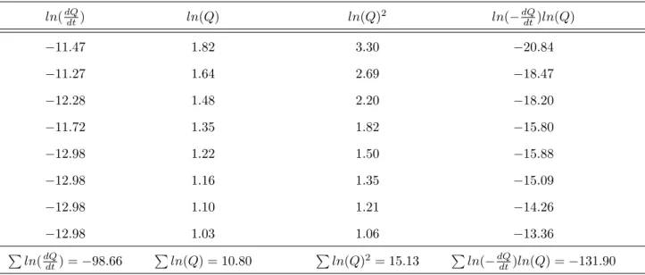
Table 4.1: Daily streamflows of first recession event of basin 03368000 t(Days) Q(t) (f t3_/sec₎ ₋dQ dt (f t 3_/sec2₎ _Q₍_{f t}3_/sec₎ _ln₍dQ dt) ln(Q) 1 6.6 1.04×10−5 _6.15 ₋₁₁_.₄₇ ₁_.₈₂ 2 5.7 1.27×10−5 _5.15 ₋₁₁_.₂₇ ₁_.₆₄ 3 4.6 4.63×10−6 4.40 −12.28 1.48 4 4.2 8.10×10−6 3.85 −11.72 1.35 5 3.5 2.31×10−6 _3.40 ₋₁₂_.₉₈ ₁_.₂₂ 6 3.3 2.31×10−6 _3.20 ₋₁₂_.₉₈ ₁_.₁₆ 7 3.1 2.31×10−6 _3.00 ₋₁₂_.₉₈ ₁_.₁₀ 8 2.9 2.31×10−6 2.80 −12.98 1.03 9 2.7

Table 4.2: Calculation ofαand k

ln(dQ_dt) ln(Q) ln(Q)2 _ln₍₋dQ dt)ln(Q) −11.47 1.82 3.30 −20.84 −11.27 1.64 2.69 −18.47 −12.28 1.48 2.20 −18.20 −11.72 1.35 1.82 −15.80 −12.98 1.22 1.50 −15.88 −12.98 1.16 1.35 −15.09 −12.98 1.10 1.21 −14.26 −12.98 1.03 1.06 −13.36 P_ln₍dQ dt) =−98.66 P_ln₍_Q_{) = 10}_.₈₀ P_ln₍_Q₎2_{= 15}_.₁₃ P_ln₍₋dQ dt)ln(Q) =−131.90

(33)

After substituting all the known values the equations 4.1, 4.2 becomes

−98.66−10.80α−8ln(k) = 0 (4.3)

−131.90−15.13α−10.80ln(k) = 0 (4.4)

Equations 4.3, 4.4 are solved for obtainingα, kof that recession event.

4.1.2 Calculation of k after fixing

α

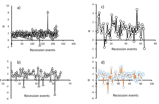
-2 0 2 4 6 8 10 0 50 100 150 200 250 300 α Recession events a) -6 -4 -2 0 2 4 6 -10 10 30 50 70 α Recession events b) -2 -1 0 1 2 3 4 0 20 40 60 80 α Recession events c) -6 -4 -2 0 2 4 6 0 20 40 60 80 100 α Recession events d)

Figure 4.1: αdistribution of the recession events during the first half of the avalaible data for the

basins (a) 03368000 (b) 08227500 (c) 011063680 (d) 014034470

Since theαvalues of the individual recession events are exhibiting static behavior (for e.g. see the

figure 4.1), to compare the variability of k across each recession eventsαof basin was fixed and k

for each recession event was calculated from the following equation 4.5.

n−1 X i=1 ln−(dQ dt)i−nln(k)−α n−1 X i=1 (ln(Q)i) = 0 (4.5)

(34)

For the same basin 03368000 and for the first recession period (αof the basin is fixed as the median

ofαdistribution of all the individual recession events and is observed as 1.83). So after fixing theα

equation 4.5 becomes

−98.66−8ln(k)−19.76 = 0 (4.6)

Thus fixing ofαenables to comparekof individual recession events.

4.1.3 Selecting of past discharge

Q

N

and k of each recession event

For each recession event for the prediction of k which is having power law relationship with past storage, past discharge of each recession event corresponding to 6,20,45,80,120 days by excluding

two days from the peak were selected. For the same basin 03368000 the past dischargeQN and k

were shown in figure 4.2.

4.1.4 Calculating the

Q

avg

by observing the trend of

Q

N

After selecting the values ofQN, in order to account the past storage which is contributing to the

recession event average ofQN upto whichQN has shown increasing trend was calculated and

repre-sented asQavg. k is function of past storage which is not a physical quantity, hence past discharge

of basin was considered as a proxy for the past storage. The above condition helps in isolating the past discharge which is equivalent to the past storage that is contributing to the recession discharge.

In other words if we blindly consider the past 120 days average discharge for the prediction ofk, it

may not contain all the past discharge that is contributing to the past storage (it may contains the surface flow).

(35)

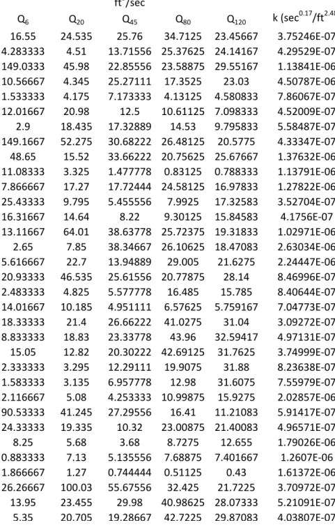
Q

₆

Q

₂₀

Q

₄₅

Q

₈₀

Q

₁₂₀

k (sec

0.17

/ft

2.48

)

16.55

24.535

25.76 34.7125

23.45667

3.75246E-07

4.283333

4.51 13.71556 25.37625 24.14167

4.29529E-07

149.0333

45.98 22.85556 23.58875 29.55167

1.13841E-06

10.56667

4.345 25.27111

17.3525

23.03 4.50787E-06

1.533333

4.175 7.173333

4.13125

4.580833

7.86067E-07

12.01667

20.98

12.5 10.61125 7.098333

4.52009E-07

2.9

18.435 17.32889

14.53 9.795833

5.58487E-07

149.1667

52.275 30.68222 26.48125

20.5775

4.33347E-07

48.65

15.52 33.66222 20.75625 25.67667

1.37632E-06

11.08333

3.325 1.477778

0.83125

0.788333

1.13791E-06

7.866667

17.27 17.72444 24.58125 16.97833

1.27822E-06

25.43333

9.795 5.455556

7.9925

17.32583

3.52704E-07

16.31667

14.64

8.22 9.30125

15.84583

4.1756E-07

13.11667

64.01 38.63778 25.72375 19.31833

1.02971E-06

2.65

7.85 38.34667 26.10625 18.47083

2.63034E-06

5.616667

22.7 13.94889

29.005 21.6275

2.24447E-06

20.93333

46.535 25.61556 20.77875

28.14 8.46996E-07

2.483333

4.825 5.577778

16.485

15.785 8.40644E-07

14.01667

10.185 4.951111

6.57625

5.759167

7.04773E-07

18.33333

21.4 26.66222

41.0275

31.04 3.09272E-07

8.833333

18.83 23.33778

43.96 32.59417

4.97131E-07

15.05

12.82 20.30222 42.69125

31.7625

3.74999E-07

2.333333

3.295 12.29111

19.9075

31.88 8.23638E-07

1.583333

3.135 6.957778

12.98 31.6075

7.55979E-07

2.116667

5.08 4.253333 10.99875

15.9275

2.02857E-06

90.53333

41.245 27.29556

16.41 11.21083

5.91417E-07

24.33333

19.335

10.32 23.00875 21.40083

4.96571E-07

8.25

5.68

3.68 8.7275

12.655 1.79026E-06

0.883333

7.13 5.135556

7.68875

7.401667

1.2607E-06

1.866667

1.27 0.744444

0.51125

0.43 1.61372E-06

26.26667

100.03 55.67556

32.425 21.7225

3.70972E-07

13.95

23.455

29.98 40.98625 28.07333

5.21091E-07

5.35

20.705 19.28667

42.7225

29.87083

4.03807E-07

8.566667

91.39 54.72667 61.52375 44.10833

7.12935E-07

2.35

1.29 0.642222

0.70375

1.1 1.8237E-06

76.11667

39.445 22.65111 13.92375

9.555 3.8772E-07

8.333333

22.76 35.39778

31.9825

23.715 4.20402E-07

7.333333

25.55 39.72889

33.9775

25.7375

3.11022E-07

3.783333

4.81 6.415556

25.14 24.81917

1.88927E-06

0.616667

2.435 3.693333 10.97375

19.345 1.48576E-06

1.516667

1.01 0.755556

0.6775

0.705833

1.08876E-06

ft

3

/sec

Figure 4.2: Average past dischargeQN and finalkfor first 33 recession events for the basin 03368000.

(36)

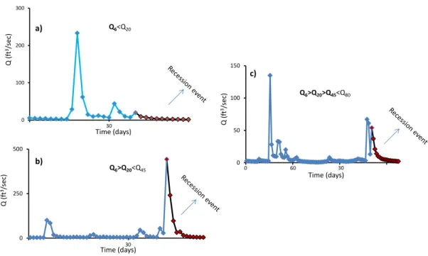
For separating the recession event and it’s storage, the possible favorable conditions are as follows 1.Q6> Q20> Q45> Q80> Q120 2.Q6> Q20> Q45> Q80 3.Q6> Q20> Q45 4.Q6> Q20 5.Q6< Q20

If it fails in the beginning (i.e.Q6< Q20)Q6 was considered asQavg.

For the basin 03368000, randomly selected values of past discharge satisfying above the conditions is shown in the table 4.3.

(37)

Table 4.3: For the basin 03368000 various possible conditions of past discharges that arises in contributing the past storage to the recession flow.

f t3

sec

Recession event Q6 Q20 Q45 Q80 Q120 Remarks

8 149.17 52.28 30.68 26.48 20.58 Q6> Q20> Q45> Q80> Q120 35 2.35 1.29 0.64 0.63 1.1 Q6> Q20> Q45> Q80 13 16.32 14.64 8.22 9.30 15.85 Q6> Q20> Q45 9 48.65 15.52 33.66 20.76 25.68 Q6> Q20 1 16.55 24.54 25.76 34.71 23.46 Q6< Q20 0 100 200 300 Q6<Q20 0 50 100 150 Q6>Q20>Q45<Q80 a) c) 0 60 30 0 250 500 Q6>Q20<Q45 b) 30 30 Time (days) Time (days) Time (days) Q ( ft 3/sec) Q ( ft 3/sec) Q ( ft 3/sec)

Figure 4.3: Involvement of surface flow after 6th_{, 20}th_{, 45}th _{day of recession events 1, 9, 13 for the}

(38)

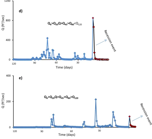
0 400 800 1200 Q6>Q20Q>Q45>Q80<Q120

d)

0 200 400

e)

Q6>Q20Q>Q45>Q80>Q120 120 90 60 30 120 90 60 30 Time (days) Time (days) Q (f t 3/sec) Q (f t 3/sec)

Figure 4.4: Involvement of surface flow after 80th, 120th day of recession events 35, 8 for the basin

03368000

Q6> Q20> Q45> Q80> Q120

It essentially indicates that there was no storm event or leakage from the surrounding aquifer that has a major contribution to the recession flow. It can be best visualized by the figure 4.4.(e). During the past discharge time series there was a sudden rise in the past flow at day 30 and 80 but their error causing probability is less due to their less lasting period. In such a case the past stream

(39)

N = 6,20,45,80,120) was considered as Qavg.

Q6> Q20> Q45> Q80

It essentially indicates that there was no storm event or leakage from the surrounding aquifer that has a major contributes to the recession flow. It can be best visualized by the figure 4.4.(d). During the past discharge time series there was a sudden rise (upto 400 cusecs) in the past flow after day 80. so if their contribution after day 80 is considered, error causing probability will be more due to their high frequency nature. In such a case the past stream flow from day 2 to 80 contributes to the

recession flow. So due to this average ofQN (whereN= 6,20,45,80) was considered asQavg.

Q6> Q20> Q45

It essentially indicates that there was no storm event or leakage from the surrounding aquifer that has a major contributes to the recession flow. It can be best visualized by the figure 4.3.(c). During the past discharge time series there was a sudden rise (upto 140 cusecs) in the past flow after day 45. so if their contribution after day 45 is considered, error causing probability will be more due to the involvement of surface flow. In such a case the past stream flow from day 2 to 45 only contributes

to the recession flow. So due to this average ofQN (whereN= 6,20,45) was considered asQavg.

Q6> Q20

It essentially indicates that there was no storm event or leakage from the surrounding aquifer that has a major contributes to the recession flow. It can be best visualized by the figure 4.3.(b). During the past discharge time series there was a sudden rise (upto 100 cusecs for two consecutive days) in the past flow after day 20. so if their contribution after day 20 is considered, error causing probability will be more due to the involvement of surface flow. In such a case the past stream flow from day

2 to 20 only contributes to the recession flow. So due to this average ofQN (whereN = 6,20) was

considered asQavg.

Q6< Q20

It essentially indicates that there was no storm event or leakage from the surrounding aquifer that has a major contributes to the recession flow. It can be best visualized by the figure 4.3.(a). During

(40)

the past discharge time series there was a sudden rise (upto 220 and 80 cusecs for two consecutive days) in the past flow after day 6. so if their contribution after day 6 is considered, error causing probability will be more due to the involvement of surface flow. In such a case the past stream flow

from day 2 to 6 only contributes to the recession flow. So due to this average ofQN (whereN = 6)

was considered asQavg.

4.1.5 Performing the linear regression analysis (

ln

converted linear

re-gression analysis) between

k

and past discharge

The constants between power law relation ofk and past discharge, (k_N0 ,λN) depends onN values

for a given basin.

n X i=1 ln(k)i−nln(k 0 N) +λN n X i=1 ln(QN) = 0 (4.7) n X i=1 ln(k)iln(QN)i−nln(k 0 N) n X i=1 ln(QN) +λN n X i=1 ln(QN)2= 0 (4.8)

Table 4.4: For the same basin the prediction ofk using the power law relation betweenkand past

dischargeQN is illustrated with the help of table given below.

Qavg k(sec

0.17

f t2.48 ) ln(Qavg) ln(k) ln(k)log(Qavg) ln(Qavg)2

16.55 3.75×10−07 ₂_.₈₁ ₋₁₄_.₈₀ ₋₄₁_.₅₉ ₇_.₉₀ 4.283 4.29×10−07 ₁_.₄₅ ₋₁₄_.₆₆ ₋₂₁_.₂₆ ₂_.₁₀ 72.62 1.14×10−06 4.29 −13.68 −58.69 18.40 7.46 4.51×10−06 2.00 −12.31 −24.62 4.00 1.53 7.86×10−07 0.43 −14.06 −6.05 0.18 12.02 4.52×10−07 ₂_.₄₉ ₋₁₄_.₆₁ ₋₃₆_.₃₈ ₆_.₂₀ 2.90 5.58×10−07 ₁_.₀₆ ₋₁₄_.₄₀ ₋₁₅_.₂₆ ₁_.₁₂ 55.84 4.33×10−07 ₄_.₀₂ ₋₁₄_.₆₅ ₋₅₈_.₈₉ ₁₆_.₁₆ 32.09 1.38×10−06 ₃_.₄₇ ₋₁₃_.₄₉ ₋₄₆_.₈₁ ₁₂_.₀₄ 3.50 1.14×10−06 ₁_.₂₅ ₋₁₃_.₆₈ ₋₁₇_.₁₀ ₁_.₅₆

(41)

k values (after fixing the value ofα) and past discharge for first 10 recession events were shown

in the above table 4.4. Here onlyQavgwas considered instead ofQN. From the table 4.4

P ln(Qavg) = 23.27 P_ln₍_k_{) =}₋₁₄₀_.₃₄ P ln(Qavg)ln(k) =−326.65 P_ln₍_Q avg)2= 69.66 After replacing (k0_N, λN) by (k 0

avg, λavg), equations 4.7, 4.8 becomes

n X i=1 ln(k)i−n ln(k 0 avg) +λavg n X i=1 ln(Qavg) = 0 (4.9) n X i=1 ln(k)iln(Qavg)i−n ln(k 0 avg) n X i=1 ln(Qavg)i+λavg n X i=1 ln(Qavg)2= 0 (4.10)

Substituting the above values in equations 4.9, 4.10

−140.34−10ln(k0_avg) + 23.27λavg= 0 (4.11)

−326.65−232.7ln(k_avg0 ) + 69.66λavg= 0 (4.12)

By solving the above equations the values ofk0_avg, λavg are computed. So by using the power law

relation betweenkandQavgthekvalue of any advance recession event can be found out.

4.1.6 Selection of regression coefficients corresponding to high strength

of determination values

Generally due to the consideration of separated past discharge for each recession event, the strength

of relationship betweenk and past discharge is larger whenQavg is considered. This behavior was

proved in 74% of the basins (see the R2 _{values of} _{kV sQ}

N and kV sQavg shown in columns 2−7

of the SM −1 provided at the end). Also in almost all of the remaining cases there exists only

(42)

to strength of relationship ofkandQavg. So for predicting thekof advancing recession eventQavg

was considered for correlating with k for all the basins. For all the basins (λavg, k

0

avg) during the

calibration period were shown in 9−10 columns of theSM−1 provided at the end.

4.1.7 Calculating the

Q

avg

for predicting the recession flow during the

validation period

In the same way as the calibration period in order to calculate the recession flow,Qavgwas calculated

by observing the trend of QN i.e. average of past average discharges upto which it has shown

increasing trend was considered.

4.1.8 Choosing the formula for predicting the dry weather flow (recession

flow)

Prediction of dry weather flow can be done by using as well as not using the initial discharge by using the following equations

Prediction of dry weather flow using the initial discharge

Qt=Q0(1 +k

0

NQN−λNt(α−1)Qα0−1)

1

1−α _(4.13)

whereQtis dry weather flow at time t

Q0is initial discharge at the beginning of the recession event

(λN, k

0

N) are power law coefficient and constant between the power law relationship betweenkand

QN.

αis the fixed value ofαdistribution of individual recession events of basin.

Due to high strength of determination betweenk andQavg (λN, k

0

N) were replaced by (λavg, k

0

avg).

The Qavg used in the above equation is belongs to validation period and should not be confused

(43)

Prediction of dry weather flow without using the initial discharge

Suppose if the recession event or dry weather period lasts for larger time period, dry weather flow can be predicted even without using the initial discharge by the following formula. In our case due to the availability of initial discharge during the validation period (second half of the data) recession flows were predicted by using both the equations 5.2, 5.3. For each prediction case the model performance was checked individually.

Qt= (k

0

NQN−λNt(α−1))

1

1−α (4.14)

4.1.9 Evaluating the model performance after calculating the dry weather

flow

(Q4)o= 0.825(Q4)m R² = -0.02 0 10 20 30 0 10 20 30 (Q4)m (cusecs) (Q 4 )o (cu se cs) a) b) (Q0)o= 1.9373(Q0)m R² = 0.65 0 100 200 0 30 60 (Q0)m (cusecs) (Q0 )o (c u secs )

Figure 4.5: Linear regression passing through origin of both the cases of predicted and observed recession flows during second half of data

(44)

(Q

4

)

o

(Q

4

)

m

(Q

4

)

m

*0.825

(Q

0

)

o

(Q

0

)

m

(Q

0

)

m

*1.9373

4.2 8.884728

3.465

45 17.36897 33.64890843

3.5 6.780311

2.8875

11 10.26025 19.87717478

3.3 5.436649

2.7225

6.7 7.117409 13.78855678

3.1 4.510592

2.5575

4.7 5.376322 10.41554814

2.9 3.836926

2.3925

4.2 4.281798 8.295127878

2.7 3.326737

2.2275

3.4 3.535395 6.849120458

2 4.116452

1.65

2.5 2.996577 5.805267959

1.8 3.141438

1.485

7.1 4.931014 9.552853655

1.7 2.518896

1.4025

4.2 3.727358 7.221011071

1.6 2.089837

1.32

3.3 2.96989

5.753568701

4.6 20.61666

3.795

3 2.452972

4.75214177

3.7 15.73344

3.0525

2.7 2.079623 4.028853035

2.7 12.61553

2.2275

2.4 1.798409 3.484057713

2.2 10.46665

1.815

2.2 1.579631

3.06021995

1.8 8.903436

1.485

66 23.69518 45.90466469

1.4 7.719562

1.155

20 13.71235 26.56493944

1.3 6.794588

1.0725

13 9.420039 18.24944184

1.1 6.053701

0.9075

9.1 7.075457 13.70728262

0.9 5.448097

0.7425

7.1 5.614144 10.87628093

0.7 5.643313

0.5775

6.8 4.623361 8.956837782

0.6 4.306651

0.495

6.5 3.911107 7.576988059

0.5 3.453197

0.4125

6.3 3.376521 6.541333955

0.3 2.864993

0.2475

13 10.43514 20.21599424

1.1 2.293948

0.9075

11 8.664404 16.78555015

1 1.750609

0.825

8.2 7.374667 14.28694334

0.8 1.403689

0.66

6.7 6.39698

12.39286909

0.6 1.16459

0.495

5.8 5.63253

10.9118998

0.4 0.990656

0.33

5.4 5.01985

9.72495492

4.2 7.404903

3.465

5 4.518792

8.75425597

Figure 4.6: Observed and predicted recession flows for the basin 03368000 for both the cases of prediction with and without considering the bias error.

(45)

In the figure 4.5, (Q4)o=observed stream flows of each recession event from day 4 without considering

the initial discharge; (Q4)m=predicted stream flows of each recession event from day 4 without

considering the initial discharge; (Q0)o=observed stream flows of each recession event from day 2

with considering the initial discharge; (Q0)m=predicted stream flows of each recession event from

day 2 with considering the initial discharge.

In this study dry weather flows were predicted by using the above formulae and the model performance was checked with the help of various model evaluation statistics like coefficient of

determination (R2_{), NSE, PBIAS (percent bias), RSR (RMSE - standardization ratio).} _Model

evaluation parameters were also calculated from predicted and observed dry weather flows after removing the bias error. In other words if we fit the linear regression passing through the origin of predicted and observed values we can see whether the model under estimates or over estimates the observed values by a certain fixed value. In such case we can remove that bias error by multiplying the predicted values with the constant of proportionality between predicted and observed values. It can be better understand by the following example. For the 03368000 predicted stream flows both by using initial discharge and not by using the initial discharge along with the first 29 observed

stream flows during the validation period (second half of the data) was shown figure 4.6. For

that basin after fitting the observed and predicted for both the cases of prediction the regression

constants passing through origin are given as 0.825 (for the prediction case without considering

initial discharge), 1.9373 (for the prediction case with considering initial discharge respectively). In

the first case of prediction the predicted recession flows indicates the over estimation of the model

by a factor 0.825, so all the predicted flows were multiplied by the same factor in order to remove

the bias error. For the later case the model under estimates the observed flows by a factor 1.9373

so all the predicted stream flows were multiplied by 1.9373 to remove the bias error. So in such way

the performance of the model was evaluated by various model evaluation statistic parameters like

coefficient of determination (R2), NSE, PBIAS (percent bias), RSR (RMSE - standardization ratio)

with the inclusive of bias error and after the elimination of bias error. For the above basin recession flows of around 2648 days were observed to be present during the validation period. The above

mentioned constants 0.825, 1.9373 were obtained by the linear regression passing through origin of

(46)

For reference purpose first 29 days observed and predicted stream flows only presented in the figure 4.6.

4.2 Relative gravity observing procedure

The following screens were edited prior to the gravity observation

In Survey screen, we have to specify the surveyor’s identifier, station designation system, station grid reference parameter etc.. In autograv screen we can enable or disable the corrections due to various factors like tide, continuous tilt, terrain. Besides this it also contain option for saving or rejecting the raw data. In Options screen, we can specify the no.of cycles, starting delay (to attain stability before measurement), measurement type (numeric or alpha characteristic). Dump screen can be used for the transferring the data in text of alpha numeric format. Using Clock and Options screen, we can set the time and date of measurement, and for customer support and calibration issues options screen can be useful.

The following steps briefly explains the observations of gravity by Scientrix-CG5 gravimeter. 1. First level the instrument at the selected station with leveling screws provided at the bottom of tripod.

2. Choose the grid reference parameters like projection datum, enable/disable the corrections and other options like number of cycles and period of each cycle for observing the gravity.

3. Finally observe the gravity at that station and repeat the same procedure at remaining stations. 4. Finally dump the data with the USB.

(47)

4.3 Station topography details and magnitudes of corrections

for elevation and latitude

Table 4.5: The following details of the stations were used in employing the major corrections. Due to lack of data, only two major corrections were employed.

Station No. Latitude N (◦) Longitude E (◦) Elevation (m) ∆gh(mGal) ∆gφ(mGal)

1 17.492911 78.135361 599.2368 184.9244765 2865.145355 2 17.492677 78.136990 608.0760 187.6522536 2865.111296 3 17.492448 78.138389 600.4560 185.3007216 2865.077964 4 17.492369 78.138949 598.6272 184.7363539 2865.066466 5 17.492354 78.139124 598.6272 184.7363539 2865.064282 6 17.492275 78.139547 598.6272 184.7363539 2865.052784 7 17.492288 78.139628 598.6272 184.7363539 2865.054676 8 17.492208 78.139998 598.6272 184.7363539 2865.043031 9 17.492208 78.140195 611.7336 188.780989 2865.043031 10 17.492113 78.140944 599.8464 185.112599 2865.029204 11 17.491893 78.142418 599.2368 184.9244765 2864.997182 12 17.491769 78.143356 597.408 184.3601088 2864.979133

(48)

Chapter 5

Results and Discussions

5.1 Results for the calibration period

This study, emphasises the recession flows which are affected by subsurface properties only, by eliminating the peaks of all the recession events which are most likely due to the surface flow. From here on wards, recession event means, its exclusive of two days inclusive of the recession peak. The analysis was also performed by excluding the last element of recession curve to exclude the influence of next storm but the difference was found to be minimal. For each study basin all the recession

events were selected and recession constantsαandkwere computed by non-linear regression analysis.

αof the basin was taken as the median of αdistribution of all the recession events. Due to its high

variability in the individual segments of the recession,kwas calculated individually for each recession

event.

Prediction of the streamflow aftertth_{day of the peak of the recession curve is mainly influenced}

bykas variation ofαof a basin is limited. According to Biswal and Kumar (2014) recession flow at

any time can be obtained by integrating the recession equation and applying the limits and resulting equation is given below.

Qt=Q0(1 +kt(α−1)Qα0−1)

1

(49)

substituting the expression ofk, the above equation becomes Qt=Q0(1 +k 0 NQN−λNt(α−1)Qα0−1) 1 1−α _(5.2)

whereQ0 is the initial discharge i.e. discharge att= 0. But for large value of time (a minimum of

4 days in a general case), recession flow is independent of initial discharge [8] and the equation 5.2 becomes Qt= (k 0 NQN−λNt(α−1)) 1 1−α (5.3)

with better estimatedkvalue for a recession event, equation 5.2 can be used for streamflow prediction

provided the initial discharge of recession event is known. Even without knowing the initial discharge, advance forecasting of dry weather flow from fourth day of the recession event can be done by using

equation 5.3. So to check the robustness of the model, streamflows were predicted from 4th_{day, 2}nd

day of each recession event during the validation period.

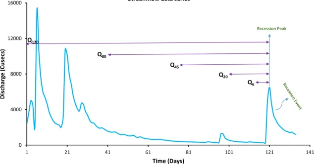
0 4000 8000 12000 16000 1 21 41 61 81 101 121 141 Di sc ha rg e (Cus ecs ) Time (Days) Streamflow data series

Recession Peak Q₆ Q45 Q20 Q₈₀ Q120

Figure 5.1: Illustrates the basic concept of the streamflow time series data in this study. The

recession parameterkwas examined with past streamflow (QN) by considering fiveN values (N=

(50)

5.2 Anomaly of recession coefficient

k

with cumulative past

discharge from a fixed reference

In Bart and Hope (2014), baseflow recession characteristics during water season for four basins

(USGS ids :11143300,1115200,11148900,11149900) of MCR (Mediterranean Climate Regions) were

analyzed. The recession ratekis inversely proportional to antecedent storage which indicates that as

the time span increases, the antecedent storage contribution towards the recession decreases [16, 8]. The difference between Biswal, Bart approach was in Biswal’s approach the average past streamflows

of 8,28,118 days were considered for each recession event whereas Bart and Hope (2014) investigated

kof each recession event with antecedent cumulative streamflow from peak of each recession event to

the beginning of corresponding water year. Similarly in our study antecedent discharge prior to the

recession event was divided into five regions, with each region commencing fromN0[2,10,30,60,100]

days toN”_[10_,₃₀_,₆₀_,₁₀₀_,_{140] days respectively (for selecting the past streamflow for each recession}

event). In Bart and Hope (2014) antecedent cumulative discharge was considered for each recession event. However, rainfall is expected to be sparsely distributed in all the 324 basins and also as the basins were not confined to any particular topography so for accounting this average discharge from

N0 days before the peak of the recession event to (N

0

+N”₎

2 days i.e past discharge corresponding to

6,20,45,80,120 days were considered for each recession event. Interestingly in Bart and Hope (2014)

analysis, the strength of the relationship ofkandQP W Y (cumulative streamflow from peak to the

beginning of the corresponding water year) was much improved compared to traditional investigation

ofkwith past streamflowQN (N = 8, 28, 118 days were adapted in Bart and Hope (2014) study).

In our analysis also the similar kind of approach was undertaken. The main difference between their analysis and our analysis was, in Bart and Hope (2014) approach irrespective of position of recession event the section for selecting the past streamflow was fixed as the beginning of the water

water whereas our study introduces a term Qavg which was taken as the average of all the past

average streamflows ofQN upto which they showed an increasing pattern i.e. if Q6≥QN (where

N = 20,45,80,120, again average of the discharges till the above sequence followed was considered

asQavg). If the sequence fails at the initial stage, 6 days average discharge before the recession was

(51)

5.3 Calibration of

k

from the proposed novel approach

For calibrating the recession parameters individual recession events from half of the available data

were selected. αand k parameters for each recession curve were computed by using nonlinear

re-gression analysis. It was observed that for all the basins α of each recession event doesn’t vary

much, whereas kwas shown an erratic behavior, which indicates that any change that takes place

in the storage characteristics that will directly reflects in k. For example, Big Sur basin (USGS

id: 11143000), has α distribution with a median value of 2.42 (with a standard error of ±0.14).

Similarly for the basins with USGS ids: 01488500,11482500,14185000,14187000 αvalues were

re-ported as 2.69, 2.25, 2.42, 2.19 respectively. Sok values were calculated for all the recession events

using non linear regression analysis after fixing α of the basin as the median of αdistribution of

individual recession events. Represented αvalues of all the basins were provided in 8th column of

the supplementary material provided.

k= 3E-08Q6-0.94 R² = 0.85 1001 ₁₀03 ₁₀05 10-08 10-10 10-12 Q6(ft3/sec) k (sec 0.4 2/ft 4.26 ) 1001 ₁₀03 ₁₀05 10-08 10-10 10-12 Q20(ft3/sec) k (sec 0.4 2/ft 4.26 ) k = 5E-08Q20-0.98 R² = 0.89 1001 ₁₀03 ₁₀05 10-08 10-10 10-12 k (sec 0.4 2/ft 4.26 ) y = 5E-08x-0.977 R² = 0.8942 k = 6E-08Qavg-1.03 R² = 0.91 1001 ₁₀03 ₁₀05 10-08 10-10 10-12 k (s ec 0.4 2/ft 4.26 ) y = 5E-08x-0.977 R² = 0.8942 y = 6E-08x-1.027 R² = 0.9054 k = 7E-08Q45-1.02 R² = 0.89 1001 ₁₀03 10-08 10-10 10-12 y = 5E-08x-0.977 R² = 0.8942 y = 6E-08x-1.027 R² = 0.9054 y = 7E-08x-1.017 R² = 0.8858 1005 k = 8E-08Q80-1.01 R² = 0.73 100 ₁₀02 ₁₀04 10-08 10-10 10-12 y = 4E-08x-0.914 R² = 0.4625 y = 4E-08x-0.914 R² = 0.4625 k = 4E-08Q120-0.91 R² = 0.46 k (sec 0.4 2/ft 4.26 ) k (sec 0.4 2/ft 4.26 ) Q45(ft3/sec) Q80(ft3/sec) Q120(ft3/sec) Qavg(ft3/sec) a b c d e f

Figure 5.2: a to e illustrates the scatter plot of QN Vs kforN = 6,20,45,80,120 days for Siuslaw

river near Mapleton (USGS id :14307620). f represents the scatter plot ofQavg Vsk. Even though

R2avg ≈R220, a substantial improvement (higherR2avg) overR2N (WhereN = 6,20,45,80,120 days

(52)

1E-08 0.0000001 0.000001 1 10 100 1000 10000 10-06 10-07 10-08 100 ₁₀01 ₁₀02 ₁₀03 1004 k = 2E-06Q6-0.42 R² = 0.51 Q6(ft3/sec) k (s ec 0.23 /f t 2.3 1) a) 1E-08 0.0000001 0.000001 1 10 100 1000 100 ₁₀01 ₁₀02 1003 10-06 10-07 10-08 Q20(ft3/sec) k (s ec 0.23 /f t 2.3 1) k = 3E-07Q20-0.45 R² = 0.47 b) 1E-08 0.0000001 0.000001 1 10 100 1000 100 ₁₀01 ₁₀02 1003 10-06 10-07 10-08 k (s ec 0.23 /f t 2.3 1) Q45(ft3/sec) k = 3E-07Q45-0.45 R² = 0.38 c) 1E-08 0.0000001 0.000001 1 10 100 1000 100 ₁₀01 ₁₀02 ₁₀03 10-06 10-07 10-08 k (s ec 0.23 /f t 2.3 1) Q80(ft3/sec) k = 2E-07Q80-0.35 R² = 0.19 d) 1E-08 0.0000001 0.000001 1 10 100 1000 100 ₁₀01 ₁₀02 ₁₀03 k = 1E-07Q120-0.20 R² = 0.06 Q120(ft3/sec) k (s ec 0.23 /f t 2.3 1) 10-06 10-07 10-08 1E-08 0.0000001 0.000001 1 10 100 1000 100 ₁₀01 ₁₀02 ₁₀03 10-06 10-07 10-08 k (s ec 0.23 /f t 2.3 1) Qavg(ft3/sec) k = 3E-07Qavg-0.48 R² = 0.53 f) e)

(53)

1E-08 0.0000001 0.000001 1 10 100 1000 10-06 10-07 10-08 10-01 ₁₀01 ₁₀02 ₁₀03 k = 7E-07Q6-0.58 R2_{= 0.70} Q6(ft3/sec) k (s ec 0.28 /f t 2.1 6) 1E-08 0.0000001 0.000001 1 10 100 1000 a) 10-06 10-07 10-08 10-01 ₁₀01 ₁₀02 ₁₀03 k = 6E-07Q20-0.55 R2_{= 0.63} Q20(ft3/sec) k (s ec 0.28 /f t 2.1 6) b) k = 2E-07Q120-0.23 R2_{= 0.75} 1E-08 0.0000001 0.000001 1 10 100 1000 10-06 10-07 10-08 10-01 ₁₀01 ₁₀02 ₁₀03 k = 5E-07Q45-0.45 R2_{= 0.42} Q45(ft3/sec) k (s ec 0.28 /f t 2.1 6) _c) 1E-08 0.0000001 0.000001 1 10 100 1000 10-06 10-07 10-08 10-01 ₁₀01 ₁₀02 ₁₀03 k = 3E-07Q80-0.32 R2_{= 0.17} Q80(ft3/sec) k (s ec 0.28 /f t 2.1 6) d) 1E-08 0.0000001 0.000001 1 10 100 10-06 10-07 10-08 100 ₁₀01 ₁₀02 Q120(ft3/sec) k (s ec 0.28 /f t 2.1 6) e) 1E-08 0.0000001 0.000001 1 10 100 1000 k = 6E-07Qavg-0.60. R2_{= 0.65} 10-06 10-07 10-08 100 ₁₀01 ₁₀02 Qavg(ft3/sec) k (s ec 0.28 /f t 2.1 6) f) 1002

river near Mapleton (USGS id :08227500). f represents the scatter plot ofQavgVs k.

For each basin, recession rate k was investigated with past streamflow (k = k0QN−λ). The

constants k0 , λwere find out by non linear regression analysis of k and QN. The scatter plot of

k and QN for the basins with USGS id 14307620, 03028000, 08227500 were shown in the figure

5.2, 5.3, 5.4. For the basin 14307620, from the coefficient of determination values R2

6 = 0.85, R2

20 = 0.89, R245 = 0.89, R280 = 0.73, R2120 = 0.46 , it was clear that the influence of antecedent

streamflow over the recession with the time decreases i.e. asN increases R2_N decreases. R2_N where

(N = 6,20,45,80,120) for all the basins were provided in columns 2−6 of supplementary material

provided.

Interestingly the strength of relationship (R2

Storage characterization through gravity-meter experiments and stream flow analysis: Consequences for dry weather flow prediction