No. 2003–62
CO-MOVEMENT, CAPITAL AND CONTRACTS:
‘NORMAL’ CYCLES THROUGH CREATIVE
DESTRUCTION
By P. Francois and H. Lloyd-Ellis
July 2003
Co—Movement, Capital and Contracts:
‘Normal’ Cycles Through Creative Destruction
Patrick Francois
CentER, Tilburg University
and
Department of Economics
University of British Columbia
[email protected]
Huw Lloyd—Ellis
Department of Economics
Queen’s University
and
CIRPÉE
[email protected]
June, 2003
AbstractWe develop a unified theory of endogenous business cycles in which expansions are neoclassical growth periods driven by productivity improvements and capital accumulation, while down-turns are the result of Keynesian contractions in aggregate demand below potential output. Recessions allow skilled labor to be reallocated to growth—promoting activities which fuel sub-sequent expansions. However, rigidities in production and contractual limitations, inherent to the process of creative destruction, leave capital severely underutilized. A key feature of our equilibrium is the endogenous emergence of long—term supply contracts between capitalist owners and producers.
Key Words: Long—term contracting, investment irreversibility, putty—clay technology, asset— specificity, Endogenous cycles and growth
JEL: E0, E3, O3, O4
Funding from Social Sciences and Humanities Research Council of Canada and the Netherlands Royal Academy of Sciences is gratefully acknowledged. This paper has benefitted from the comments of Paul Beaudry and David R. F. Love and seminar participants at UBC, UWO, the 2003 Midwest Macroeconomics Conference and the 2003 meetings of the Canadian Economics Association meetings. The usual disclaimer applies.
“The recurring periods of prosperity of the cyclical movement are the form progress takes in capitalistic society.” (Joseph Schumpeter, 1927)
1
Introduction
A defining feature of thenormal business cycle is the observed co—movement across diverse sectors of the economy amongst both outputs and inputs to production.1 Indeed, sectoral co—movement in output was one of the key characteristics discussed in the work of Burns and Mitchell (1946), and forms the basis for the NBER’s business cycle dating methodology.2 Recently, Christiano and Fitzgerald (1998) have documented the striking degree of co—movement in labor hours across highly disaggregated sectors of the US economy. This sectoral co—movement has long been recog-nized, at least informally, by macroeconomists. For example, Schumpeter (1927) argued that the key to understanding business cycles was to understand why entrepreneurial activity would be clustered over time. Similarly, Keynes (1936) emphasized the role of co—movement in investment behavior – encapsulated in his notion of “animal spirits” – as a key causal factor in the business cycle.
Despite these observations, mainstream macroeconomic analysis has, in recent decades, tended to put aside questions regarding thecauses of co—movement and, instead, has largely focussed on the propagation mechanisms implied by various aggregate shocks. In particular, the real business cycle literature emphasizes the response of the economy to aggregate technology shocks in driving short—run fluctuations. However, while technology shocks may be important at the firm level, it is not obvious why they would be important for economy—wide aggregate output fluctuations. As Lucas (1981) reasons, positive technology shocks for some firms would surely be offset by negative shocks for others. Even if one were to accept the existence of aggregate technology shocks as a driving force in the co—movement of outputs across sectors, standard RBC models still have trouble explaining the observed co—movement ininputs across sectors. In particular, as has been pointed out recently (Christiano and Fitzgerald, 1998, Siu, 1999), standard RBC models imply that hours worked in the consumption goods sector are inherentlycounter—cyclical.3
1In using the expression “normal business cycle” we are borrowing from Schumpeter (1927, p. 288), who distinguishes such cycles from seasonalfluctuations, “long waves” and secular trends.
2“... a recession is a period of decline in total output, income, employment, and trade, usually lasting from six months to a year, and marked by widespread contractions in many sectors of the economy.” (see http://www.NBER.org/cycles.html).
There are, however, good reasons why economic activity might be correlated across different industries, even in the absence of aggregate shocks. In the presence of imperfect competition, for example, the implementation of a productivity improvement by one firm may increase the demand for anothers’ products by raising aggregate demand. In a dynamic general equilibrium setting, Shleifer (1986) shows that this may induce innovators, who anticipate short-lived profits, to implement simultaneously, thereby generating self—enforcing booms in activity. Unfortunately, as a vehicle for understanding actual business cycles, Shleifer’s model suffers from a number of serious limitations. Firstly, the multiplicity of equilibria that arise yield rather imprecise predictions for the cyclical process. Secondly, the temporary nature of profits relies on the ad hoc assumption of drastic, but costless imitation. Thirdly, his cycle features only booms and slowdowns, but no downturns. Finally, Shleifer’s theory depends critically on the impossibility of any type of storage (including physical capital).4
In Francois and Lloyd-Ellis (2003), we demonstrate how a similar endogenous cyclical process can arise through a process of “creative destruction” familiar from Schumpeterian growth models. Like imitation, potential obsolescence limits the longevity of profits and provides incentives to cluster implementation. We show that when productive resources are needed to generate new innovations, allowing for the possibility of storage does not rule out cycles, and in fact yields a
unique cyclical equilibrium.5 Moreover, because this costly innovation tends to be clustered just before a boom, it causes a downturn in aggregate output (even if the measure of GDP includes this investment). Although promising, our earlier model allowed investment only in intangible
assets (i.e. “ideas”). This limits its applicability becausefluctuations intangiblecapital formation (and its utilization) are, obviously, a key characteristic of the business cycle.6
The omission of physical capital from our earlier paper was not innocuous. If consumption— smoothing households have access to fully reversible and continuously variable physical capital, they would “eat” it in anticipation of a boom, thereby undermining the existence of cycles where delay plays an important role. As Matsuyama (1999) notes, this is true more generally of work develop extended RBC frameworks in which hours worked in the consumption sector need not be counter-cyclical. As will be seen this problem need not arise in our framework either. We discuss this issue in Section 7.
4If they could, innovators would choose to produce when costs are low (i.e. before the boom), store the output and then sell it when demand is high (i.e. in the boom). Such a pattern of production would undermine the existence of cycles.
5Shleifer (1986) assumes that innovations arise exogenously. When innovation is endogenous, growth is inti-mately related to the business cycle.
6A related limitation of that model is that for realistic long—run growth rates, the existence of the cyclical equilibrium requires unrealistically high values of the elasticity of intertemporal substitution of 3 or above.
featuring agglomeration with implementation delay (Shleifer 1986, Deneckere and Judd 1992, and Gale 1996). The results of such models are not robust to allowing the accumulation of (fully reversible) physical capital. Matsuyama’s (1999, 2001) resolution of this impasse is to develop a model of endogenous cycles with physical capital, but without implementation delays. His model features increasing returns in production (as in Romer, 1990), exogenous imitation (as in Shleifer, 1986), and afixed entry cost for newfirms. This results in a growth process in which the economy fluctuates between periods of high capital accumulation coupled with low total factor productivity (TFP) growth, and periods of high TFP growth but little accumulation of capital. While this model is useful as a tool for understanding longer term phenomena (e.g. East Asian post war growth and the US productivity slowdown), it has a number of shortcomings when applied to business cycle frequency fluctuations. In particular, sectoral contractions in output – a key aggregate feature of normal business cycles – are absent from this process. Similarly, consumption never actually falls in absolute terms and factors of production are always fully utilized.7
Here we consider an alternative approach that allows for physical capital, but preserves the implementation delays emphasized by previous authors. Specifically, we develop a model of innovation—driven endogenous growth in which capital is irreversible, putty-clay and lumpy. Our emphasis on the rigidities of installed capital is consistent with our focus on normal business cycles rather than secular trends and, as we will demonstrate, generates dynamics that are quali-tatively consistent with key features of the data at this frequency. Moreover, there is considerable direct evidence that many types of physical investment are not reversible and feature putty-clay characteristics (see Ramey and Shapiro, 2001, Kasahara, 2002). Doms and Dunne (1993) have also documented the considerable “lumpiness” of plant level investments, while Cabellero and Engel (1998) have demonstrated the high skewness and kurtosis observed in aggregate invest-ment data.8 Moreover, the variation in “shiftwork” over the business cycle (see Bresnahan and Ramey 1994, Hamermesh 1989 and Mayshar and Solon, 1993) is consistent with the putty—clay assumption, since it implies that capital is being used less intensively during recessions than is 7There is a large literature on endogenous cycles and growth. However, most previous work has been restricted to single sector settings, which also seems more consistent with the analysis of general purpose technologies and longer term, secular trends. See Aghion and Howitt (1998, ch. 8) and Lloyd-Ellis and Francois (2003) for more extensive discussions of this literature.
8
A related literature emphasizes the role of plant level investment irreversibilities. However, recent work (see Veracierto, 2002 and Thomas 2002,) in the RBC tradition has found that the effects of such irreversibilities at the aggregate level are virtually non—existent.
optimal ex ante.
We characterize an endogenous stationary cyclical equilibrium that features dramatic shifts in economy—wide investment behavior through the cycle. Expansions are “neoclassical”, supply— side phenomena which directly raise bothpotential output, through the delayed implementation of productivity improvements, and actual output through increased labor effort and subsequent capital accumulation. Recessions are “Keynesian” demand—side contractions during which ac-tual output falls below its potential and some capital resources are left under—utilized. These reductions in aggregate demand are not autonomous, however. Rather they are an equilibrium response to the anticipated future expansion, as effort shifts into long—run growth promoting activities, and out of current production.9
In addition to an endogenous treatment of growth, our model endogenously generates the following qualitative behavior of key aggregates and prices over the business cycle:
• Implementation of innovations is strongly pro—cyclical, so that total factor productivity rises during booms, but remains constant during downturns.
• Labour productivity is strongly pro—cyclical.
• Wages rise during booms and expansions, but do not fall during contractions.
•Investment and consumption are strongly pro—cyclical, but investment is more volatile. Invest-ment is strongly correlated with output and sales growth.
• Labor and capital inputs into consumption and investment sectors are both pro—cyclical. • Capacity utilization is strongly pro—cyclical.
• Profits are strongly pro—cyclical.
• Term spread isflat during expansions and steep midway through contractions.
• Marginal Q is strongly pro—cyclical, but because the stock market anticipates the boom, the cyclicality of Tobin’s average Qtends to be more complex.
A crucial feature of the equilibrium growth path that we study is the endogenous emergence of optimal long term supply contracts between capital owners (e.g. banks) and entrepreneurs. Contractual agreements negotiated between the two parties are necessarily limited because the process of creative destruction implies that an entrepreneur’s productivity advantage terminates when replaced by superior innovators in their sectors.10 The parties can, however, enter into long 9This has theflavor of the so—called “paradox of thrift”: current savings are chanelled into investments whose return will not be realized until the long run (when, according to Keynes (1936), “we are all dead”).
1 0
The growth implications of incomplete contracting have been explored recently in a number of papers: Marti-mort and Verdier (2000) explore the growth implications of cooperative non-productive behavior between owners
term binding arrangements that specify both the quantity and price of capital to be transacted, conditional upon the relationship continuing. As we shall see, the existence of contracts between intermediate producers and capital suppliers, also precipitates the emergence of contracts between final goods producers and their intermediate suppliers.
We defer discussion of previous literature on growth and cycles until after the paper’s main results are presented. The paper proceeds as follows: Section 2 sets out the framework, Section 3 characterizes the cycling steady state, Section 4 presents the necessary conditions for existence of the steady state and Section 5 provides numerical examples of cycling economies, and comparative statics. Section 6 deals with the model’s dynamics and Section 7 concludes with a discussion of the main implications. All proofs are in the Appendix.
2
The Model
2.1
Assumptions
There is no aggregate uncertainty. Time is continuous and indexed byt≥0. We consider a closed economy with no government sector. The representative household has isoelastic preferences
U(t) = Z ∞ t e−ρ(τ−t)C(τ) 1−σ −1 1−σ dτ (1)
where ρ denotes the rate of time preference and σ represents the inverse of the elasticity of intertemporal substitution. The household maximizes (1) subject to the intertemporal budget constraint Z ∞ t e−[R(τ)−R(t)]C(τ)dτ ≤S(t) + Z ∞ t e−[R(τ)−R(t)]w(τ)dτ (2) where w(t) denotes wage income, S(t) denotes the household’s stock of assets (firm shares and capital) at time t and R(t) denotes the discount factor from time zero to t. The population is normalized to unity and each household is endowed with one unit of labor hours, which it supplies inelastically.
Final output can be used for the production of consumption, C(t),investment, K˙(t), or can be stored at an arbitrarily small flow cost of ν >0 per unit time. It is produced by competitive firms according to a Cobb—Douglas production function utilizing a continuum of intermediates, and workers. Francois and Roberts (2002) show that the productivity slowdown, and a number of accompanying labor market changes can be explained in an endogenous growth framework featuring such incomplete contracting. Acemoglu, Aghion and Zilibotti (2002,2003) explore the implications for such incompleteness for LDC development.
xi,indexed by i∈[0,1]: C(t) +K˙(t)≤Y(t) = exp µZ 1 0 lnxi(t)di ¶ . (3)
For simplicity we also assume that there is no physical depreciation.
Output of intermediate i depends upon the state of technology in sector i, Ai(t), utilized
capital,Kiu(t),which cannot exceed the stock of installed capital, Ki(t), and labor hours, Li(t),
according to the following putty—clay technology:
xsi(t) = ½ [Ku i(t)] α[A i(t)Li(t)]1−α whereKiu(t) =Ki(t) κi(z)αAi(t)1−αLi(t) whereKiu(t) =κi(z)Li(t)< Ki(t) (4) where κi(z) is the capital—labor ratio chosen at z < t, the time at which the last increment
to capital was installed. The unit measure of labor hours is perfectly mobile across sectors and inelastically supplied by households in aggregate. However, the amount of this supply that is used in production of intermediates potentially varies due to its opportunity cost in an alternative activity, specified shortly. Installed capital,Ki(t), is sector—specific and is owned by “capitalists”
who rent it to entrepreneurs at the rateqi(t). Installed capital is non-divisible so that any part
of it that is not utilized cannot be used elsewhere.11 Once installed, sector—specific capital is irreversible,K˙i ≥0,as well as putty-clay. We assume that intermediates are completely used up
in production, but can be produced and stored for use at a later date. Incumbent intermediate producers must therefore decide whether to sell now, or store and sell later at the flow storage cost ν.
An implication of this structure is that during an expansion, when new capital is being built, firms can choose (K, L) combinations along the Cobb—Douglas production isoquants (curved in Figure 1) and choose an optimal capital—labor ratio that reflects relative factor prices. However during a contraction, if labor is removed and the firm produces below capacity, production must utilize factors along a ray from the chosen point on the full-capacity isoquant, which reflects the same factor ratios. In such a situation, the installed capital is used less intensively in proportion to the labor hours allocated to production. One interpretation of this is that there are fewer shifts.
This production set up implies that if firms were to reduce output below capacity, one of the following three outcomes must occur:
1 1
For similar examples of putty-clay capital, see Johansen (1959), Gilchrist and Williams (2000) and Kasahara (2003). Evidence of underutilization is widespread: for example, Bils and Cho (1994) and Basu (1996).
(1) the entire stock of capital is rented to another (presumably more productive) entrepreneur, if one exists;
(2) capital is fully utilized, but some output is stored to be sold later, or (3) the installed capital remains in place but is under—utilized, Kiu(t)< Ki(t).
Along the cyclical growth path that we will study here, only outcome (3) turns out to be consistent with equilibrium. However, we will discuss in some detail the conditions that rule out (1) and (2). κ(z) contraction (t>z) expansion (t<z) K L
Figure 1: Implications of Irreversibility and Putty—Clay Technology
2.1.1 Innovation
Competitive entrepreneurs in each sector attempt to find ongoing marginal improvements in productivity by allocating labor effort to innovation rather than production.12 Theyfinance their activities by selling equity shares to households. The probability of an entrepreneurial success in instant tis δHi(t), where δ is a parameter, and Hi is the labor effort allocated to innovation in
sector i. At any point in time, entrepreneurs decide whether or not to allocate labor effort to innovation, and if they do so, how much. The aggregate labor hours allocated to innovation is given byH(t) =R01Hi(t)dt.
1 2All of the labor considered here is skilled and capable of substituting between the two activities. We discuss the implications of allowing unskilled labor in the concluding section.
New ideas and innovations dominate old ones by a factor eγ. Successful entrepreneurs must
choose whether or not to implement their innovation immediately or delay implementation until a later date.13 Once they implement, the knowledge associated with their improvement becomes publicly available, and can be built upon by rival entrepreneurs. However, prior to implementa-tion, the knowledge is privately held by the entrepreneur.14 We let the indicator function Zi(t)
take on the value 1 if there exists a successful innovation in sector i which has not yet been implemented, and 0 otherwise. The set of instants in which entrepreneurial successes are imple-mented in sector i is denoted by Ωi. We let ViI(t) denote the expected present value of profits
from implementing a success at time t, andViD(t) denote that of delaying implementation from timet until the most profitable time in future.
2.1.2 Contracts
The nature of innovation is such that entrepreneurs cannot simply “sell” their ideas to capitalists, but must be involved in its implementation themselves. We assume that entrepreneurs do not have the wealth required to purchase the capital stock needed to implement, and hence must borrow from the capitalists. In effect, there is a separation of ownership and control with respect to the capital stock of thefirm, which may necessitate the writing of a long—term capital supply contract. The effective user cost of capital is the outcome of such a contractual relationship between the entrepreneur and the capitalists in each sector. Incumbent capital owners are limited in the extent of their monopoly pricing by the threat of “replacement” capital being built in their sector.15
Capital Supply Contracts: Intermediate producers and capital owners in every sector i can
contract over a future binding utilized capital level, Kiu(τ),and a price for each unit of utilized capital,qi(τ), for all τ up to a chosen contract termination date, TiK.Thus a contract signed at
time t is a tuplen{Kiu(τ), qi(τ)}τ∈[t,TK i ], T
K i
o
.16 Since the productive advantage of an inter-1 3
As in Francois and Lloyd—Ellis (2003) we adopt a broad interpretation of innovation. Recently, Comin (2002) has estimated that the contribution of measured R&D to productivity growth in the US is less that 1/2 of 1%. As he notes, a larger contribution is likely to come from unpatented managerial and organizational innovations.
1 4Even for the case of intellectual property, Cohen, Nelson and Walsh (2000) show thatfirms make extensive use of secrecy in protecting productivity improvements. Secrecy likely plays a more prominent role for entrepreneurial innovations, which are the key here.
1 5
In order to maintain competition in capital supply it will be assumed that, in the event of a competing capital stock being built, ties in tended prices are always broken in favour of the entrant. Due to storage costs, entry of replacement capital will imply scrapping of the pre-existing stock.
1 6
Identical results obtain if instead of specifying the time-varying utilization rate of capital, Kiu(τ), contracts can only be written overK(τ).
mediate producer lasts only until a superior technology is implemented in that sector, contracts allow the termination of agreements before TK
i if shutting down production. Otherwise, the
parties can break contracts only by mutual agreement.
Although supply contracts with particular entrepreneurs only last until their ideas become obsolete, capitalist owners can retain their incumbency permanently (subject to competition from other capitalists). The present value of the capitalist’s net income in sector i under the utilization—price sequence {Kiu(τ), qi(τ)}∞τ=t is therefore:
ViK(t) = Z ∞ t e−[R(τ)−R(t)]hqi(τ)Kiu(τ)−K˙i(τ) i dτ . (5)
Intermediate Supply Contracts: Final goods producers are also able to contract intermediate
good deliveries from each of the intermediate producing sectors, i. Such contracts written at t
involve a similar tuple: n{xi(τ), pi(τ)}τ∈[t,TX i ], T
X i
o
where the unit price is pi(t) and the
contract termination date isTiX.Contracts can be altered under the same conditions as in capital contracts.17 The value of final goods producers is denotedVY(t).
2.2
De
fi
nition of Equilibrium
Given initial state variables18 {Ai(0), Zi(0), Ki(0)}1i=0,an equilibrium for this economy is:
(1) a sequence of capital supply contracts ½ b TK iv, n b Ku i (t),qbi(t) o t∈[TbK iv−1,TbivK] ¾ v∈I ,
(2) a sequence of intermediate supply contractsnTbivX,{bxi(t),pbi(t)}t∈[TbX iv−1,TbivX]
o
v∈I,
(3) sequences nKbi(t), Lbi(t), Hbi(t), Abi(t), Zbi(t), VbiI(t), VbiD(t), VbiK(t)o
t∈[0,∞) for each
inter-mediate sectori, and (4) economy wide sequences
n b
Y(t), Rb(t), wb(t), VbY (t), Cb(t), Sb(t)
o
t∈[0,∞)
which satisfy the following conditions:
• Households allocate consumption over time to maximize (1) subject (2). The first—order con-ditions of the household’s optimization require that
b
C(t)σ =Cb(τ)σeRb(t)−Rb(τ)−ρ(t−τ) ∀ t, τ , (6) and that the transversality condition holds
lim τ→∞e
−Rb(τ)Sb(τ) = 0 (7)
1 7
Though conceptually feasible, contracts written over the supply of labor andfinal output are redundant in the equilibria we study and will not be considered further.
1 8
• Labor markets clear:
Z 1 0
b
Li(t)di+Hb(t) = 1 (8)
•Arbitrage trading infinancial markets implies that for all assets that are held in strictly positive amounts by households, the rate of return between timetand time smust equal Rb(ss)−−Rtb(t). • Free entry into innovation – entrepreneurs select the sector in which they innovate so as to maximize the expected present value of the innovation, and
δmax[VbiD(t),VbiI(t)]≤wb(t), Hbi(t)≥0 with at least one equality. (9)
• At instants where there is implementation, entrepreneurs with innovations must prefer to im-plement rather that delay until a later date
b
ViI(t)≥VbiD(t) ∀t∈Ωbi. (10)
• At instants where there is no implementation, either there must be no innovations available to implement, or entrepreneurs with innovations must prefer to delay rather than implement:
EitherZbi(t) = 0, (11)
or ifZbi(t) = 1, VbiI(t)≤VbiD(t) ∀ t /∈Ωbi.
• For all capital supply contracts written at date t, the equilibrium contract is such that no other contract dominates for the capitalist and all existing entrepreneurs indexed by technologies
Ai(τ)≤Ai(t) in sectori: max h b ViI(t),VbiD(t) i +VbiK(t) ≥ max£ViI(t), ViD(t)¤+ViK(t) (12) ∀mutually determined ViJ 6= VbiJ, J =I, D, K. (13)
•For all intermediate supply contracts written at datet,the equilibrium contract is such that no other contract dominates for thefinal goods producer and all existing entrepreneurs in sector i:
maxhVbiI(t),VbiD(t)i+VbY (t) ≥ max£ViI(t), ViD(t)¤+VY (t), (14) ∀mutually determined ViJ 6= VbiJ, J =I, D, K, (15)
whereVY (t) holds contracts with other intermediate suppliers fixed. • Free entry intofinal output production: VbY (t)≤0
3
The Acyclical Balanced Growth Path
In this section, we briefly consider the existence of an equilibrium growth path along which the utilized capital offirms grows monotonically, entrepreneurship is continuous and implementation is never delayed. We derive the equilibrium without utilizing long—term contracts, so that all transactions occur in spot markets, since it will be seen that allowing for them does not affect the equilibrium. While the acyclical growth path is not our main focus, it is useful for understanding our later results.
Consumption satisfies the familiar differential equation:
˙
C(t)
C(t) =
r(t)−ρ
σ , (16)
where r(t) =R˙(t), denotes the continuous time interest rate.In the absence of uncertainty or adjustment costs, and as long as utilized capital is anticipated to grow, capitalists never acquire more capital than is needed for production, so that
Kiu(t) =Ki(t). (17)
Within each sector,i,the existence of potential capital entrants implies that capital owners cannot earn excess returns on marginal units. Hence:
Lemma 1 : As long as new capital is being built, free—entry into capital markets implies that
qi(t) =q(t) =r(t) ∀ i. (18)
Final goods producers choose intermediates to maximize profits, taking their prices as given. The derived demand for intermediate iis
xdi(t) = Y(t)
pi(t)
. (19)
The unit elasticity of demand for intermediates implies that limit pricing, which drives out the previous incumbent, is optimal:
Lemma 2 : The limit price is given by
pi(t) = q(t)αw(t)1−α µe−(1−α)γA1−α i (t) . (20) where µ=αα(1−α)1−α.
The resulting instantaneous profit earned in each sector is given by
π(t) = (1−e−(1−α)γ)Y(t). (21)
Aggregate final output can be expressed as
Y(t) = [K(t)]α£A(t)L(t)¤1−α, (22)
where A(t) = exp³R01lnAi(t)di´. Along the acyclical steady—state growth path, a constant fraction of the labor force is allocated to entrepreneurship. The standard solution method yields the following steady state implication:
Proposition 1 : If
(1−e−(1−α)γ)γ(1−σ) 1−αe−(1−α)γ <
ρ
δ (23)
then there exists an acyclical equilibrium with a constant growth rate given by
ga= max " [δ(1−e−(1−α)γ)−ρ(1−α)e−(1−α)γ]γ 1−αe−(1−α)γ−γ(1−σ) (1−α)e−(1−α)γ,0 # . (24)
Along this equilibrium growth path, the inequality in (23) implies that r(t) > ga(t) at every moment. Along a balanced growth path, this condition must hold for the transversality condition to be satisfied and hence for utility to be bounded. However, this condition also ensures both that no output is stored, and that the implementation of any innovation is never delayed (see Francois and Lloyd—Ellis, 2003, for further elaboration). Allowing long—term supply contracts would only undermine the existence of this equilibrium growth path if contracting for non-spot market prices could make both parties to a contract better off. However, since all quantities are chosen optimally in the spot market in this equilibrium, such contracts would necessarily involve one side being made worse off.
4
The Posited Cyclical Growth Path
In this section, we begin by informally positing a cyclical equilibrium growth path in which, due to the rigid nature of capital, under—utilization may occur during downturns. We then posit the equilibrium behavior for capitalists and entrepreneurs over the cycle and detail the implications for contracting, consumption and aggregate entrepreneurship. In Section 5, we derive more formally the implications of this behavior over each phase of the cycle, and Section 6 then demonstrates
the consistency of the posited behavior of entrepreneurs and capitalists in an equilibrium steady state and derives the conditions for existence.
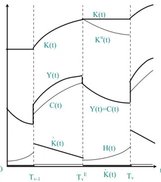
t K(t) Y(t) C(t) K(t) Tv-1 TvE Tv Ku(t) 0 H(t) . Y(t)=C(t) K(t) K(t).
Figure 2: Evolution of Key Aggregates over the Cycle
Figures 2 and 3 depict the movement of key variables during the cycle. Cycles are indexed by the subscriptv,and feature a consistently recurring pattern through their phases. The vth cycle features three distinct phases:
•Theexpansionis triggered by a productivity boom at timeTv−1 and continues through
subse-quent capital accumulation, leading to continued growth in output, consumption and wages. Over this expansion phase the interest rate falls and investment, though positive, declines as the capi-tal stock rises. Also, since labor’s productivity in manufacturing intermediates is relatively high, no labor is allocated to entrepreneurship. Through time, continued capital accumulation lowers returns to further investment, rendering entrepreneurship relatively more attractive. Eventually innovation and reorganization re-commence, drawing labor hours from production. At this point, the return on investment in physical assets drops to zero, and investment ceases temporarily.
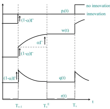
•Thecontractionstarts with a collapse infixed capital formation at timeTvEas investment shifts
aggre-t Tv-1 TvE Tv 0 w(t) q(t) r(t) pi(t) (1-α)Γ (1-α)Γ (1-α)Γ αΓ no innovation innovation
Figure 3: Evolution of Prices over Cycle
gate demand and then optimally re-allocate resources to relatively labor intensive entrepreneurial reorganization in order to raise productivity for the forthcoming boom. Due to irreversibility and the putty-clay nature of installed capital, labor’s departure from production implies that capital cannot be fully utilized. Through the downturn, capital utilization falls and is traded at a constant price. Innovation and reorganization continue to increase throughout this phase so that the economy continues to contract through declining consumption expenditure.
• The boom occurs at an endogenously determined date, Tv, when the value of implementing
stored innovations first exceeds the value of delaying their implementation. At that point, all entrepreneurs implement their successful innovation, starting the upswing once again. During the boom the returns to production rise above those of innovation and re—organization, drawing skilled labor out of entrepreneurship and into production. Returns to capital also rise with the new more productive technologies, so that capital accumulation recommences and the cycle begins again.
4.1
Contracts
Because competition from replacement capitalists weakens during a recession, contracts arise endogenously as capitalists compete to offer guaranteed prices to capital users in advance of the downturn. At this point, we anticipate the form these contracts will take and derive their implications. In Section 6 we shall verify that these contracts are constrained optimal given these implications. Contracts are written during the expansion of each cycle and terminate just before the boom of the next. Contracts between intermediate andfinal goods producers specify a sequence of quantities and prices for intermediates through the cycle. These contracted prices reflect the marginal costs of the main competitor: the previous incumbent holding the next best technology. The prices and quantities agreed to in the intermediate goods contract take the same form as the spot market values along the acyclical growth path:
pci(t) = q(t) αw(t)1−α µe−(1−α)γA1−α i (Tv−1) ∀t∈[Tv−1, Tv). (25) xci(t) = Y (t) pc i(t) ∀t∈[Tv−1, Tv). (26)
Through the upturn, contracts between capitalists and entrepreneurs specify steady expan-sion in each sector’s capital stock, with capital being traded at a declining market—clearing price. During a contraction, the contracts specify afixed rental price for capital and a declining utiliza-tion rate. The equilibrium contracts are written beforeTvE−1 over rental rate and utilized capital {qic(t), Kic(t), Tv} and take the following form:
qci(t) = ( αe−(1−α)γA1−α(Tv−1)K(t)α−1 ∀ t∈ £ Tv−1, TvE ¤ αe−(1−α)γA1−α(Tv−1)K(TvE)α−1 ∀ t∈(TvE, Tv) (27) Kic(t) = ½ K(t) ∀ t∈£Tv−1, TvE ¤ λ(t)K¡TvE¢ ∀ t∈(TvE, Tv), (28) whereλ(t)<1denotes the utilization rate. Note that the posited contracts are symmetric across sectors. In fact, as we will see, a contract specifying a constant price through the downturn is not necessary. What will be required is that the price sequence is such that its average equals a unique value. However, a constant price with this property is an equilibrium, and if there is any arbitrarily small cost to price adjustment it is unique.
4.2
Consumption
Over intervals during which the discount factor does not jump, consumption is allocated as described by (16). However along the cyclical growth path, the discount rate jumps at the boom, so that consumption exhibits a discontinuity during implementation periods. We therefore characterize the optimal evolution of consumption from the beginning of one cycle to the beginning of the next by the difference equation
σln C0(Tv)
C0(Tv−1)
=R(Tv)−R(Tv−1)−ρ(Tv−Tv−1). (29)
where the 0 subscript is used to denote values of variables the instant after the implementation boom. Note that a sufficient condition for the boundedness of the consumer’s optimization problem is that ln C0(Tv)
C0(Tv−1) < R(Tv)−R(Tv−1) for allv, or that
(1−σ)
Tv−Tv−1
ln C0(Tv)
C0(Tv−1)
< ρ ∀v. (30)
In our analysis below, it is convenient to define the discount factor that will be used to discount from some timetduring the cycle to the beginning of the next cycle. This discount factor is given by β(t) =R(Tv)−R(t) =R(Tv)−R(Tv−1)− Z t Tv−1 r(s)ds. (31)
4.3
Innovation
Let Pi(s) denote the probability that, since time Tv, no entrepreneurial success has been made
in sectoriby times. It follows that the probability of there being no entrepreneurial success by time Tv+1 conditional on there having been none by time t, is given by Pi(Tv+1)/Pi(t). Hence,
the value of an incumbentfirm in a sector where no entrepreneurial success has occurred by time
tduring thevth cycle can be expressed as
ViI(t) = Z Tv+1 t e− Rτ t r(s)dsπi(τ)dτ+Pi(Tv+1) Pi(t) e −β(t)VI 0,i(Tv+1). (32)
Thefirst term here represents the discounted profit stream that accrues to the entrepreneur with certainty during the current cycle, and the second term is the expected discounted value of being an incumbent thereafter.
Lemma 3 In a cyclical equilibrium, successful entrepreneurs can credibly signal a success imme-diately and all entrepreneurship in their sector will stop until the next round of implementation.
In the cyclical equilibrium, entrepreneurs’ conjectures ensure no more entrepreneurship in a sector once a signal of success has been received, until after the next implementation. The expected value of an entrepreneurial success occurring at some time t ∈ ¡TvE, Tv¢ but whose
implementation is delayed until time Tv is thus:
ViD(t) =e−β(t)V0I,i(Tv). (33)
Since no implementation occurs during the cycle, the entrepreneur is assured of incumbency until at leastTv+1. Incumbency beyond that time depends on the probability that there has not been
another entrepreneurial success in that sector up until then.19 The symmetry of sectors implies that entrepreneurial effort is allocated evenly over all sectors that have not yet experienced a success within the cycle. This clearly depends on some sectors not having already received an entrepreneurial innovation, an equilibrium condition that will be imposed subsequently (see Section 6). Thus the probability of not being displaced at the next implementation is
Pi(Tv) = exp à − Z Tv TE v e Hi(τ)dτ ! , (34)
where Hei(τ) denotes the quantity of labor that would be allocated to entrepreneurship if no entrepreneurial success had occurred prior to timeτ in sectori. The amount of entrepreneurship varies over the cycle, but at the beginning of each cycle all industries are symmetric with respect to this probability: Pi(Tv) =P(Tv) ∀i.
5
The Three Phases of the Cycle
5.1
The (Neoclassical) Expansion
We denote the improvement in aggregate productivity during implementation period Tv (and,
hence, the growth in the average unit cost) bye(1−α)Γv,where
Γv = ln £ Av/Av−1 ¤ , (35) 1 9
A signal of further entrepreneurial success submitted by an incumbent is not credible in equilibrium because incumbents have incentive to lie to protect their profit stream. No such incentive exists for entrants since, without a success, profits are zero.
and Av = exp
³R1
0 lnAi(Tv)di
´
. Following an implementation boom, the state of technology in use remains unchanged for the rest of the cycle. An implication of the Cobb—Douglas structure is that, through competition, the unit factor price index simply reflects this level of technology.
Lemma 4 : The input price index for t∈[Tv−1, TvE]is constant and uniquely determined by the
level of technology
q(t)αw(t)1−α =µe−(1−α)γA1v−−α1. (36)
As a result of the boom, wages rise rapidly. Since the next implementation boom is some time away, the present value of engaging in entrepreneurship falls below the wage, δVD(t) < w(t). During this phase, no labor is allocated to entrepreneurship and no new innovations come on line. However, final output grows in response to capital accumulation financed from household savings. In equilibrium the Euler equation and aggregate resource constraint imply dynamics that are almost identical to those of the Ramsey model:20
Proposition 2 During the expansion, capital and consumption evolve according to:
˙ C(t) C(t) = αe−(1−α)γAv1−−α1K(t)α−1−ρ σ (37) ˙ K(t) =A1v−−α1K(t)α−C(t). (38)
Since all capital is utilized, Lemma 1 applies so that
r(t) =q(t) =αe−(1−α)γA1v−−α1K(t)α−1. (39) Thus, as capital accumulates, the interest rate declines. Since technology is unchanging, Lemma 4 implies the wage must be rising
˙ w(t) w(t) =− µ α 1−α ¶ ˙ q(t) q(t) =α ˙ K(t) K(t) >0 (40)
During the expansion, the expected value of entrepreneurship,δVD(t), is necessarily growing at the rate of interest, but continues to be dominated by the wage in production. After enough capital has been accumulated, however, δVD(t) eventually equals w(t). At this point, if all workers were to remain in production, returns to entrepreneurship would strictly dominate those in production. As a result labor hours are re—allocated from production and into innovation, which triggers the contractionary phase.
2 0
Note that, unlike the Ramsey model, the rate of return on savings is not equal to the marginal product of capital, but rather is a fraction e−(1−α)γ of it. This reflects the entrepreneurial share of this marginal product accruing as a monopoly rent.
5.2
The (Keynesian) Contraction
Because of the putty—clay nature of capital, as labor starts to be withdrawn from production the capital—labor ratio cannot be adjusted fromκ(TvE) and output must contract. Since technology is alsofixed during this phase, the wage must be constant:
Lemma 5 : The wage for t∈[TvE, Tv]is constant and determined by the level of technology and
the capital—labor ratio chosen at the last peak, κ(TE v ):
w(t) = ¯wv = (1−α)e−(1−α)γA
1−α
v−1κ(TvE)α. (41)
Since there is free entry into entrepreneurship, w(t) = δVD(t), so that the value of en-trepreneurship, δVD(t), is also constant. Since the time until implementation for a successful
entrepreneur is falling and there is no stream of profits, because implementation is delayed, the instantaneous interest rate necessarily equals zero. If it were not, entrepreneurial activity would be delayed to the instant before the boom. Therefore:
r(t) = V˙ D(t) VD(t) = ˙ w(t) w(t) = 0. (42)
Note that this zero interest rate is consistent with the fact there is now excess (under—utilized) capital in the economy. Since marginal returns to capital in this phase are zero, physical invest-ment ceases and the only investinvest-ment is that in innovation, undertaken by entrepreneurs.
Lemma 6 : At TvE, investment in physical capital falls discretely to zero and entrepreneurship
jumps discretely to H0(TvE)>0.
A switch like this across types of investment is also a feature of the models of Matsuyama (1999, 2001) and Walde (2002). However, here factor intensity differences between entrepreneur-ship and investment lead to a crash in output followed by continued decline through the recession. Although investment falls discretely at t =TvE, consumption must be constant across the tran-sition between phases because the discount factor does not change discretely. With putty—clay technology, the decline in output due to the fall in investment demand is proportional to the fraction of labor hours withdrawn from production. It follows that the fraction of labor hours
allocated to entrepreneurship at the start of the downturn,H0(TvE),which we denote asHv from
now on, equals the rate of investment at the peak of the expansion:
Hv = ˙ K¡TE v ¢ Y (TE v ) = 1− C ¡ TE v ¢ A1v−−α1K(TE v )α . (43)
Although consumption cannot fall discretely at TE
v , the zero interest rate implies that
consump-tion must be declining afterTvE,21
˙ C(t) C(t) = r(t)−ρ σ =− ρ σ, (44)
as resourcesflow out of production and into entrepreneurship.
Since Y (t) =C(t), the growth rate in the hours allocated to production is also given by (44) and so aggregate entrepreneurship at time tis given by
H(t) = 1−(1−Hv)e−
ρ σ[t−T
E
v]. (45)
Note that the putty—clay nature of capital implies that as labor leaves current production, capital utilization falls in the same proportion. It follows that the capital utilization rate specified in the equilibrium contract (28) is given by
λ(t) = (1−H0(TvE))e−
ρ
σ(τ−TvE). (46)
During the downturn, in the absence of a capital contract, entrepreneurs would be vulnerable to an increasing rental price through the downturn. To see why, observe that, in order to forestall entry by a competing capitalist, the incumbent capitalist is constrained to offer a price—quantity sequence which satisfies
VK(K(t), t) =
Z Tv
t
e−[R(τ)−R(t)]hq(τ)Ku(τ)−K˙(τ)idτ+e−β(Tv)VK(K(t), T
v)≤K(t), (47)
where VK(K(t), τ) denotes the value of the installed capital at time τ. During the downturn
r(t) = 0 andK˙(τ) = 0,so that for t∈£TvE, Tv
¤
,the condition becomes: Z Tv t q(τ)λ(τ)K(TvE)dt+e−β(Tv)VK¡K(TE v ), Tv ¢ ≤K(TvE). (48)
However competition from potential replacement capitalists at the beginning of the next cycle ensures thatVK¡K(TE
v ), Tv
¢
=K(TE
v ). Dividing byK(TvE) and re—arranging, using (46), yields
a necessary restriction to forestall entry during the downturn: Z Tv t q(τ) (1−Hv)e− ρ σ(τ−T E v)dτ ≤1−e−β(Tv). (49)
The right hand side of this expression is constant throughout the downturn, but the left—hand side would be decreasing through the downturn if q(t) were constant. It follows that, in the absence of a contracted price, the capitalist could raise q through the downturn and still satisfy
(49).
The main implication of this is that, without a contract written beforeTvE delineating the price charged by the capitalist for the remainder of the cycle, entrepreneurs will face an increasing rental rate for capital through the downturn. Given the potential for such price gouging, entrepreneurs will demand the writing of such contracts beforeTvE,when the cost of replacement capital is low.
The first thing to note about any such contract is that it must satisfy the capital feasibility constraint above, which will bind at t=TvE:
Lemma 7 Any capital supply contract {qic(τ), Kiu(τ)} signed at some date t ∈[Tv−1, TvE) must
satisfy: Z Tv TE v qc(τ) (1−Hv)e−ρσ(τ−T E v)dτ = 1−e−β(Tv) (50)
There are a number of price sequences qc(t) that could satisfy this condition, however the
average level of prices throught∈[Tv−1, TvE) is unique. Let this average in thevth cycle be
qv ≡ RTv TE v q c(τ) (1−H v)e− ρ σ(τ−T E v )dτ RTv TE v (1−Hv)e −ρσ(τ−TvE)dτ . (51)
Using 50, and integrating the denominator through the downturn,∆E
v,this implies: qv= 1−e −β(Tv) (1−Hv) µ 1−e−σρ∆Ev ρ/σ ¶. (52)
A further feature of such contracts is that they must induce a cost minimizing capital/labor ratio, in order again to forestall entry by competing capital providers. The standard marginal condition applies at every instant through the upturn. With putty/clay capital and zero dis-counting through the downturn, it is possible to treat the whole of the contractionary phase as if
it were a single production period. Consequently, a condition analogous to the standard marginal condition applies to the optimal capital/labor ratio through the downturn,
(1−α)K¡TvE¢ αL(TE
v )
= wv
qv.
Since,L¡TvE¢= 1,it follows that:
Proposition 3 For a capital—supply contract to be efficient through the downturn it is necessary
that capital is installed only up to the point at which the marginal return to capital is equal to its average rental price:
q(TvE) =αe−(1−α)γA1v−−α1K(TvE)α−1 =q. (53)
Equating (52) and (53), substituting for 1 − Hv using (43), it follows that the capital—
consumption ratio at the height of the expansion can be expressed as:
K¡TvE¢ C(TE v ) = αe−(1−α)γ µ 1−e−ρσ∆Ev ρ/σ ¶ 1−e−(1−α)Γv . (54)
Note thatK¡TvE¢is also the effective capital stock at the beginning of the next boom since there is no depreciation and no capital is accumulated through the recession.
5.3
The Boom
Productivity growth at the boom is given byΓv = (1−P(Tv))γ, whereP(Tv)is defined by (34).
Substituting in the allocation of labor to entrepreneurship through the downturn given by (45) and letting
∆Ev =Tv−TvE, (55)
yields the following implication.
Proposition 4 : In an equilibrium where there is positive entrepreneurship only over the interval
(TvE, Tv], the growth in productivity during the succeeding boom is given by
Γv =δγ∆Ev −δγ(1−Hv) Ã 1−e−σρ∆ E v ρ/σ ! . (56)
For an entrepreneur who is holding an innovation, VI(t) is the value of implementing imme-diately. During the boom, for entrepreneurs to prefer to implement immediately, it must be the case that
V0I(Tv)> V0D(Tv), (57)
recalling that 0 subscripts denote values immediately after implementation. Just prior to the boom, when the probability of displacement is negligible, the value of implementing immediately must equal that of delaying until the boom:
δVI(Tv) =δVD(Tv) =w(Tv). (58)
From (57), the return to entrepreneurship at the boom is the value of immediate (rather than delayed) incumbency. It follows that free entry into entrepreneurship at the boom requires that
δV0I(Tv)≤w0(Tv). (59)
The opportunity cost offinancing entrepreneurship is the rate of return on shares in incumbent firms in sectors where no innovation has occurred. Just prior to the boom, this is given by the capital gains in sectors where no entrepreneurial successes have occurred;
β(Tv) = log µ V0I(Tv) VI(T v) ¶ . (60)
Note that since the short—term interest rate is zero over this phase,β(t) =β(Tv),∀t∈(TvE, Tv).
Combined with (58) and (59) it follows that asset market clearing at the boom requires
β(Tv)≤log µ w0(Tv) w(Tv) ¶ = (1−α)Γv. (61)
Free entry into entrepreneurship ensures that β(Tv)>(1−α)Γv cannot obtain in equilibrium.
Provided thatβ(t)>0, households will never choose to storefinal output from within a cycle to the beginning of the next either because it is dominated by the long—run rate of return on claims to future profits. However, unlikefinal output, the return on stored intermediate output in sectors with no entrepreneurial successes is strictly positive, because of the increase in its price that occurs as a result of the boom. Even though there is a risk that the intermediate becomes obsolete at the boom, if the anticipated price increase is sufficiently large, households may choose to purchase claims to intermediate output rather than claims tofirm profits.
If innovative activities are to be financed at timet, it cannot be the case that households are strictly better offbuying claims to stored intermediate goods. In sectors with no entrepreneurial
success, incumbent firms could sell such claims, use them to finance greater current production and then store the good to sell at the beginning of the next boom when the price is higher. In this case, since the cost of production is the same whether the good is stored or not, the rate of return on claims to stored intermediates in sectoriis logpi,v+1/pi,v = (1−α)Γv.
It follows that the long run rate of return on claims to firm profits an instant prior to the boom must satisfy
β(Tv)≥(1−α)Γv. (62)
Free—entry into arbitrage ensures that β(Tv)<(1−α)Γv cannot obtain in equilibrium. Because
there is a risk of obsolescence, this condition implies that at any time prior to the boom the expected rate of return on claims to stored intermediates is strictly less thanβ(t).
Combining (61) and (62) yields the following implication of market clearing during the boom for the long—run growth path:
Proposition 5 Asset market clearing at the boom requires that
β(Tv) = (1−α)Γv. (63)
Asset market—clearing thus yields a unique relationship between the discount applied over the boom, and productivity growth.22
The growth in output at the boom exceeds the growth in productivity for two reasons: first labor is re—allocated back into production, and second the previously unutilized capital is now being used productively. Since just before the boom, both inputs are a fraction (1−Hv)e−
ρ σ∆
E v
of their peak levels, output growth through the boom is given by
∆lnY(Tv) = (1−α)Γv+ (1−α)∆lnL+α∆lnKu = (1−α)Γv+ ρ σ∆ E v −ln(1−Hv) (64)
It follows directly from Proposition 5 that growth in output exceeds the discount factor across the boom. Since profits are proportional to output, this explains why firms are willing to delay implementation during the downturn.
2 2Shleifer’s (1986) model featured multiple expectations—driven steady state cycles. Such multiplicity cannot occur here because, unlike Shleifer, the possibility of storage that we allow forces a tight relationship betweenΓv and∆E
v as depicted in Proposition 4.Since Γv,∆Ev pairs must satisfy this restriction as well, in general, multiple solutions cannot be found. This however does not rule out cycles of a qualitatively different nature to those analyzed here.
The boom in output can be decomposed into a boom in consumption and investment. From the Euler equation, we can compute consumption growth across the boom:
∆lnC(Tv) = (1−α)
σ Γv. (65)
Notice that whether the growth in consumption exceeds the growth in productivity at the boom, depends on the value of σ. In particular, ifσ < 1, consumption growth must exceed aggregate productivity growth. Finally, since in the instant prior to the boom C(Tv) = Y(Tv), it follows
that the investment rate at the boom jumps to
˙ K0(Tv) Y0(Tv) =³1−(1−Hv)e( 1−σ σ )(1−α)Γv− ρ σ∆ E v ´ (66)
6
Optimal Behavior During the Cycle
Given the dynamics implied above, in this section we derive conditions which must be satisfied in order for the posited behavior of capitalists and entrepreneurs to be optimal.
6.1
Optimal Entrepreneurship and Implementation
Equilibrium entrepreneurial behavior imposes the following requirements on our hypothesized cycle:
• Successful entrepreneurs at time t = Tv must prefer to implement immediately, rather than
delay implementation until later in the cycle or the beginning of the next cycle:
V0I(Tv)> V0D(Tv). (E1)
• Entrepreneurs who successfully innovate during the downturn must prefer to wait until the beginning of the next cycle rather than implement earlier and sell at the limit price:
VI(t)< VD(t) ∀t∈(TvE, Tv) (E2)
•No entrepreneur wants to innovate during the slowdown of the cycle. Since in this phase of the cycleδVD(t)< w(t), this condition requires that
δVI(t)< w(t) ∀t∈(0, TvE) (E3)
The conditions on the value functions above take as given that entrepreneurs do not produce in excess of current demand and store their output until the boom. Provided that the incumbent
entrepreneur does not terminate the capital supply contract, (63) ensures that storage across the boom is not optimal. However, since in the posited equilibrium the capital stock is being under—utilized, it is possible that just before the boom a rival entrepreneur who has successfully innovated may be able to “buy out” the contract and utilize all the capital, meeting the current demand for output and storing the remainder until the boom.
This rival would not benefit from taking over the capital contract of the incumbent under identical terms. From (63), producing output and storing it until the boom is not optimal if he must pay a constant amountq¯for capital. Moreover, under (E2) implementation and sale before the boom is not optimal. However, the rival may be willing to take-over the use rights if able to pay q for the amount Kc(t) as in the incumbent’s contract, and utilize extra units of idle
capital at some price q < q.e Clearly any q >e 0 for the excess units would be amenable to the capitalist. The most the rival will be willing to pay per period for the current capital isqK(TvE), since e−β(Tv)q(T
v) = q. To buy out the contract, the rival must compensate the incumbent for
the loss of profits sustained for the remainder of the cycle and must offer the capitalist at least the payment he is currently receiving,q(1−Hv)e−ρσ(t−T
E v)K(TE
v )per period. It follows that such
a contract buy—out will not a be mutually acceptable at timetif Z Tv t π(τ)dτ+ Z Tv t (1−Hv)e−σρ(τ−T E v)dτ ≥ Z Tv t qK(TvE)dτ . (67)
The following proposition provides a sufficient condition for this to hold throughout the downturn:
Proposition 6 : If (1−(1−α)e−(1−α)γ)(1−Hv)e− ρ σ∆ E v > αe−(1−α)γ (E4)
then entrepreneurs who successfully innovate during the downturn prefer to wait until the be-ginning of the next cycle rather than displace the incumbent, produce now and store until the boom.
In effect, condition (E4) explains how it is possible for there to be under—utilized capital during a recession even though there exist rivals who could potentially use the capital stock more profitably. The reason is that the capital stock is “lumpy”, so that the rival cannot use a part of it while the incumbent continues to produce. For this reason the rival must compensate the
incumbent for his profit loss and this “endogenous”fixed cost is too large for entry to be profitable under recessionary demand conditions. Entry does not become profitable until the boom. There, demand is high and entry costs low because the previous incumbent’s profits do not need to be compensated as they have already been destroyed by the implementation of a superior production process.
Note finally that in constructing the equilibrium above we have implicitly imposed the re-quirement that the downturn is not long enough that all sectors innovate. Thus the following condition must be satisfied with strict inequality:
P(Tv)>0. (E5) Taken together conditions (E1) through (E5) are restrictions on entrepreneurial behavior that must be satisfied for the cyclical growth path we have posited to be an equilibrium. However, we must first check that under these conditions, the contracts we have specified are indeed undomi-nated.
6.2
The Optimality of Contracts
6.2.1 The Intermediate Good Supply Contract
The need for an intermediate contract arises because the lumpiness and sector specificity of installed capital implies that only one intermediate producer can use the sector’s capital. Though it is possible to commission the building of a new capital stock, if guaranteed a sufficiently high rental rate, the rental rate so required increases through the cycle, so that the threat of entry provides progressively weaker restraint through time. By negotiating a contract before the downturn, bids from the previous intermediate producer force limit pricing by the current incumbent at a relatively low marginal cost, since at this time the cost of building replacement capital is relatively low. Thus the intermediate goods contract guards the final goods producers against the increasing monopoly power of the incumbent through the downturn by pinning the producer down to a price/quantity pair while the previous incumbent’s threat of entry is greatest.
Lemma 8 The contracted price sequence for intermediate i, pci(t), and quantity xci(t), for t ∈
[Tv−1, Tv), satisfying (25) and (26) is optimal, given a sequence of input prices w(t), q(t) for
The input price for labor,w(t)is determined in the per period spot market so it remains now to determine the sequence of capital prices.
6.2.2 The Capital Supply Contract
The aim of capital supply contracts is to forestall hold-up by the capitalist, but the contract’s “reach” is limited on the entrepreneur’s side. Unlike capital which is infinitely lived, entrepreneurs lose their productive advantage when displaced by superior producers, so that they cannot make unconditional promises to purchase capital into the indefinite future. All contracts are thus contingent upon the entrepreneur’s continuing production. We show now that the earlier posited contract comprising (27)and (28)is an optimal response to the posited behavior of other agents over the cycle:
Proposition 7 Provided (E1)—(E5) hold then, in each sector i, at the boom of every cycle (Tv,
v = 1...∞), an equilibrium contract for the capitalist and leading entrepreneur is a sequence of prices qc(t) and capital Kc(t) for all t∈[Tv, Tv+1) that satisfies (27) and (28).
Note that the cyclical equilibrium is supported by the limitations on contracting that we have imposed. The critical, and we think realistic, assumption is that only future prices and quantities can be contracted ex ante. Allowing for a richer set of contracting possibilities would overturn this result. The sort of environments required would need to allow that, in addition to a time varying priceq and quantity K for capital, it would be possible to condition transfers between the parties on other actions that they or other parties take. For example if the new incumbent entrepreneur (who arrives probabilistically in the downturn) could somehow be party to the contract at timeTv,then full utilization of the capital through the downturn could also be
contracted ex ante. Such a rich contracting environment, however, seems to require unrealistically complex and difficult to observe details to be enforceable between the parties. Thus endogenous underutilization, which corresponds to that observed in actual business cycles, arises here due to seemingly natural limitations in contracting.
7
The Stationary Cyclical Growth Path
Here we characterize the stationary cyclical growth path implied by Propositions 2 to 5. To allow a stationary representation, we normalize all aggregate by dividing byA¯v−1 and denote the result
with lower case variables.
First recall from Proposition 2, that the dynamics of the economy during the expansion are analagous to those in the Ramsey model without technological change. Let cv = c(TvE) and
kv = k(TvE) denote the normalized values of consumption and capital at the peak of the vth
expansion. Given initial valuesc0(Tv−1)andk0(Tv−1),and an expansion length∆Xv ,it is possible
to summarize the expansion as follows:
cv = f(c0(Tv−1), k0(Tv−1),∆Xv ) (68)
kv = g(c0(Tv−1), k0(Tv−1),∆Xv ), (69)
wheref(·)and g(·) are well—defined functions.Since capital accumulation stops in the recession, and A rises by eΓv−1, it follows that k
0 = e−Γv−1kv−1. From (44), consumption declines by a
factor e−ρσ∆ E
v−1 in the recession. When combined with its increase at the boom, from (65),this yieldsc0 =e( 1−α σ −1)Γv−1− ρ σ∆ E v−1cv
−1.Substituting for c0 andk0 then yields
cv = f(e( 1−α σ −1)Γv−1− ρ σ∆ E v−1c v−1, e−Γv−1kv−1,∆Xv ) (70) kv = g(e( 1−α σ −1)Γv−1− ρ σ∆ E v−1c v−1, e−Γv−1kv−1,∆Xv ). (71)
Substituting for 1−Hv in Proposition4using (43), we can express the size of the boom as
Γv =δγ∆Ev −δγ cv kα v à 1−e−σρ∆ E v ρ/σ ! , (72)
Propositions 5 and 3 yield
αe−(1−α)γcv kv = 1−e −(1−α)Γv µ 1−e−σρ∆Ev ρ/σ ¶. (73)
Finally, asset market clearing over the boom (conditions (58)to(61))imply:
δv0I(cv, cv−1, kv, kv−1,Γv,Γv−1,∆Ev,∆Xv ) =
w0(Tv−1)
Av−1
= (1−α)e−(1−α)γe−αΓv−1kα
v−1, (74)
wherev0I =V0I(Tv−1)/A¯v−1 is explicitly derived in the appendix.
these on the equations above, yields a system offive equations in thefive unknowns: Γ = δγ∆E−δγ c kα Ã 1−e−σρ∆ E ρ/σ ! (75) αe−(1−α)γkα−1 c kα = 1−e−(1−α)Γ ³ 1−e−ρσ∆E ρ/σ ´ (76) c = f(e(1−σα−1)Γ− ρ σ∆ E c, e−Γk,∆X) (77) k = g(e(1−σα−1)Γ− ρ σ∆ E c, e−Γk,∆X) (78) δv0I(c, k,Γ,∆E,∆X) = (1−α)e−(1−α)γe−αΓkα. (79)
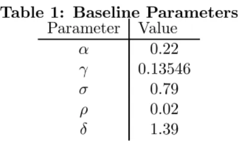
We demonstrate existence of the stationary cycle, and analyze this system numerically in the next section. However, the dynamics of the model can be understood heuristically from the phase diagram in Figure 4. Here the process of capital accumulation in the expansionary phase,
t∈¡Tv−1, TvE
¢
,within a cycle, when in steady state, is depicted.
c=C/A k=K/A k=0 c=0 . A B C k(TE) c(TE) c0 k0 S
Figure 4: Phase Diagram
The economy does not evolve along the standard stable trajectory of the Ramsey model terminating at the steady state, S. Instead, the evolution of the cycling economy during the expansion is depicted by the path betweenAandBin thefigure. Capital is accumulated starting at the pointk0 corresponding to pointA in the diagram, according to(37) and (38).The point
k0denotes the inherited capital stock at the boom. Accumulation ends atk
¡
TE¢, at which point investment stops until the next cycle. Note that if allowed to continue along such a path the economy would eventually violate transversality, but capital accumulation stops and consumption declines so that the economy evolves from B to C through the downturn. During this phase, the dynamics of the economy are no longer dictated by the Ramsey phase diagram. When this phase ends, implementation of stored productivity improvements occurs at the next boom, and
¯
A increases, so that k fall discretely. Ifσ <1, consumption grows by more than productivity at the boom, so that c rises discretely. The boom is therefore depicted by the dotted arrow back to pointA. At this point, investment in the expansionary phase recommences for the next cycle. The connection between the two phases of the cycle arises due to the allocation of resources to entrepreneurship. This allocation of resources will be reflected in the size of the increment toA,¯
Γ.
7.1
Existence of the Stationary Cycle
To demonstrate the existence of the stationary cycle, we numerically solve the model for various combinations of parameters and check the existence conditions (E1)—(E5). We choose parameters to fall within reasonable bounds of known values, and present a baseline case given in Table 1:
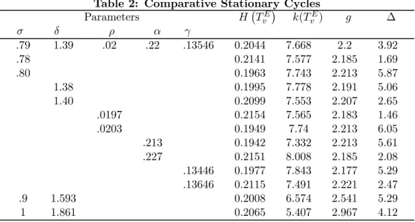
Table 1: Baseline Parameters
Parameter Value α 0.22 γ 0.13546 σ 0.79 ρ 0.02 δ 1.39
The parametersαandγwere chosen so as to obtain a labor share of0.7, a capital share of0.2and a profit share of 0.1. These values correspond approximately to those estimated by Atkeson and Kehoe (2002). The value of γ corresponds to a markup rate of around 15%. The intertemporal elasticity of substitution σ1 is slightly high, but we solve for various values below, includingσ = 1. Givenσ= 0.79, we calibratedδ andρso as to match a long—run annual growth rate of 2.2% and an average risk—free real interest rate of 3.8%, values which correspond to annual data for the post—war US. The baseline case above yields a cycle length of a little less than 4 years,Hv =.2044,