Student and School Performance Across
Countries: a Machine Learning Approach.
Chiara Masci
\, Geraint Johnes
], Tommaso Agasisti
∗January 8, 2018
\MOX - Modelling and Scientic Computing, Department of Mathematics,
Politecnico di Milano, via Bonardi 9, Milano, Italy [email protected]
]LUMS - Lancaster University Management School,
Lancaster, LA1 4YX, United Kingdom [email protected]
∗Politecnico di Milano, School of Management,
via Lambruschini 4/b, Milano, Italy [email protected]
Abstract
In this paper, we develop and apply novel machine learning and sta-tistical methods to analyse the determinants of students' PISA 2015 test scores in nine countries: Australia, Canada, France, Germany, Italy, Japan, Spain, UK and USA. The aim is to nd out which student characteris-tics are associated with test scores and which school characterischaracteris-tics are associated to school value-added (measured at school level). A specic aim of our approach is to explore non-linearities in the associations be-tween covariates and test scores, as well as to model interactions bebe-tween school-level factors in aecting results. In order to address these issues, we apply a two-stage methodology using exible tree-based methods. We rst run multilevel regression trees in the rst stage, to estimate school added. In the second stage, we relate the estimated school value-added to school level variables by means of regression trees and boosting. Results show that while several student and school level characteristics are signicantly associated to students' achievements, there are marked dierences across countries. The proposed approach allows an improved description of the structurally dierent educational production functions across countries.
Keywords: Education; Multilevel model; School value-added; Regression trees; Boosting.
1 Introduction
The educational activity involves a complex process whereby inputs (such as human and nancial resources) are converted into outputs. By analogy with the type of production function that is typically used to analyse the technology of a rm, the labour and capital inputs used by a school are likely to inuence its output. But, since students themselves form both an input and output, and since they themselves are transformed by the experience of education, such a simple framework fails adequately to capture some key salient features of the process. This is a very well-known challenge in the existent literature about Educational Production Function (EPF). Indeed, the learning process of stu-dents is inuenced by stustu-dents' own characteristics, those of their family, their peers, the neighbourhood in which they live, as well as by the characteristics of the school that they are attending. Moreover, the way in which various inputs (at dierent levels) aect output is likely to vary substantially across the edu-cational systems that operate in dierent countries. A common characteristic of all educational systems is the hierarchical structure in which students are nested within classes, that are nested within schools, that are in turn nested within cities and so forth. Establishing the structure of such a hierarchy is a non-trivial exercise, not least because this structure may be dierent across countries. Exploring international datasets which contain information about students' performance in more countries can be a rational approach to under-stand how the dierences among educational systems can have an impact on students' results, all else equal (see [16]).
The Programme for International Student Assessment (PISA) is a triennial international survey (started in 2000) which aims to evaluate education systems worldwide by testing the skills and knowledge of 15-year-old students. In 2015 over half a million students, representing 28 million 15-year-olds in 72 countries and economies, took the internationally agreed two-hour test. Students were assessed in science, mathematics, reading, collaborative problem solving and nancial literacy. Moreover, a wide array of data concerning a set of student and school levels characteristics are available, thanks to questionnaires completed by students and school principals.
Our aim in this paper is to identify which are the student and school level characteristics that are related to students' achievement, with the aim of in-vestigating the impact of these characteristics on the outcome. We analyse the school systems of nine large developed countries: Australia, Canada, France, Germany, Italy, Japan, Spain, UK, USA. Specically, our research questions are:
• Which student level characteristics are related to student achievement? • How much of the total variability in student achievement can be explained
by the dierence between schools and how can we estimate the school value-added?
in what way?
• How do co-factors interact with each other in determining outcomes
si-multaneously?
• How do these relationships between inputs/covariates and outputs/test
scores vary across countries?
In order to address these issues, we run a two stage-analysis, that departs from traditional EPFs approach and embraces a Machine Learning strategy:
1. In the rst stage, we apply multilevel regression trees (RE-EM tree, see [36]) in which we consider students (level 1) nested within schools (level 2). By means of this model we can both analyse which are the student level variables that are related to student achievements and estimate the school value-added, as a random eect (grouping factor in the hierarchical model).
2. In the second stage, we apply regression trees and boosting to identify which are the school level characteristics related to school value-added (estimated at rst stage), how they are related with the outcome and how they interact among each other.
The set of analytical tools that we use to examine these issues is new to the literature, but is quickly gaining in popularity. Tree-based methods can be classied as a Machine Learning (ML) approach. The main dierence between statistical and ML approaches is that while the former starts by assuming an appropriate data model and then estimates the parameters from the data, the latter avoids starting with a data model and rather uses an algorithm to learn the relationships between the response and the predictors (in our setting, students' test scores and their determinants, respectively). Furthermore, ML approach assumes that the data-generating process is complex and unknown and tries to identify the dominant patterns by observing inputs and the responses (see [9]). Tree-based methods (extended to accommodate the multilevel context) t the problem in hand well for several reasons. First of all, this methodology takes into account the hierarchical structure of data. The two levels of analysis are students (level 1) that are nested within schools (level 2) and it is worth disen-tangling the portions of variability explained at each level. Multilevel models are well suited to this. Secondly, our tree-based methodology does not force any particular functional form on the input-output relationship, and it allows for in-teractions among the predictors. This point is essential because the functional form of the relationships between the covariates and the outcome is unknown a priori and forcing it to be linear can considerably bias the results and, crit-ically, it does not allow discovery of the most likely relationships between the variables. Moreover, there are reasons to believe that the educational context is intrinsically characterised by interactions among variables, since inputs are various and coexist in the same environment. So, tree-based models, that are
able to let the variables interact and that identify which interactions are rel-evant in inuencing the outcome, are denitely attractive (see [23]). Thirdly, the method allows a clear graphical representation of the results that helps in communicating them to policy practitioners. Alongside the deep interrogation of interactive eects, we consider this to be a major benet of this approach.
The remainder of the paper is organised as follows: in Section 2 we review the existing literature and, in so doing, motivate our model choice; in Section 3 we present the PISA dataset and the countries that we analyse; Section 4 discusses the methodological approach (multilevel trees and boosting); in Sec-tion 5 we report the results and in SecSec-tion 6 we derive conclusions and policy implications1.
2 Background and previous literature
In recent decades, many researchers have studied the determinants of student achievement, in order to develop policy implications aimed at improving ed-ucational systems across the world. The statistical methods proposed by the literature in this perspective are various - including linear regression, multilevel linear models and stochastic frontier analysis - in each case aimed at parame-terising the educational production function (EPF). While a complete literature review of previous studies that use a EPF approach is beyond the scope of this paper, we report important points from existing contributions that can be con-sidered as relevant for interpreting our approach. Specically, we focus on those studies which adopt a cross-national perspective in modelling the determinants of students' educational performance by means of economic models and sta-tistical and econometric empirical tools. Indeed, our main contribution to the academic literature stems from the relevance of the innovations brought by the ML strategy to explore dierences in educational production across countries.
The Programme for International Student Assessment (PISA) was initiated by the OECD, and has been running since 2000. It involves standardised test-ing of 15 year olds across a large number of countries. Over the 15 years for which data are now available, PISA results have revealed that there are big discrepancies across education systems. The data allow direct comparisons of student performance in science, reading and mathematics, leading to a rank-ing of the countries and identifyrank-ing those that score the best results (see [24]). PISA2015 data, for example, show that Singapore achieves the best results in the scientic area, followed by Japan, Estonia, Finland and Canada. For our purposes, the most interesting aspect of the PISA data is the possibility that they oer to compare the marginal eects of student and school levels variables on students' performance. Gender, immigrant status, socio-economic status (SES), proportion of disadvantaged students, school size and characteristics of the school principal are all variables that have been found to be very important in some countries but less so in others (see [26] and [38]). For example, in almost
1All analysis undertaken in this paper is conducted using the statistical software R (see [29]).
all countries boys perform on average better than girls in the scientic subjects, with the notable exception of Finland, where girls have on average higher results than boys. As another example, after accounting for socio-economical status, immigrant students have a double probability compared to their not immigrant counterparts to achieve low results in scientic subjects (see [27]). Focusing on mathematics, four Asian countries outperform all other economies - Singapore, Hong Kong (China), Macao (China) and Chinese Taipei - and Japan is the strongest performer among all the OECD countries.
Policy responses to internationally reported PISA results have diered among participating countries. For example, in some country groups PISA decits have been associated with a push towards more centralised control, while others have responded with much more focused reforms implemented with the specic aim of raising PISA (or similar) test scores over time (see [42]).
What is clear to experts and analysts worldwide, therefore, is that the ed-ucational systems, in their structural, internal complexity and in their various aspects, vary within and across countries. Dierent variables play a role and sometimes with dierent impacts in inuencing educational results in dierent contexts. Analysing international datasets like PISA therefore calls for the use of a exible model, able to identify the signicant variables within each system and to t data with dierent patterns. Indeed, imposing the same coecient on the correlation between covariates and educational results in all countries is inappropriate and even the inclusion of country xed-eects - shifting only the intercept - is not obviously an adequate solution. Therefore, it is necessary to employ more exible instruments for the analysis of patterns that go beyond the simply xed-eects which impose homogeneity of the interactions between key variables within countries.
The EPF literature builds upon the work of Coleman, Hanushek, and others by viewing education as a process in which students' performance or output (attainment or years of schooling completed) is produced from inputs including school resources, teacher quality, family attributes, and peer quality. Because outcomes cannot be changed by at, policy attention has focused on inputs. These include inputs that are both directly controlled by policymakers (charac-teristics of schools, teachers, curricula, etc.) and those that are not so controlled (family, friends, the learning capacities of the student, etc.) (see [14]). While a large part of the eect on students' attainments is due to these uncontrolled characetristics of students (see [7]), many researchers have found that schools' and teachers' characteristics are also of importance in determining outcomes (see, for example, [15], [3], [32] and [43]).
In this paper, we try to nd out which are the inputs that are related with students' performances (output) and in our perspective, three main points need to be taken into account when modelling the educational production functions:
• Data levels of grouping: educational data have a hierarchical structure and
it is important to distinguish and disentangle the portion of variability in student achievements due to dierent levels of grouping ( between and within classes and schools).
• Realistic assumptions: since the educational system is a complex and
un-known process, the model assumptions are a sensitive issue and are one of the main weak points of the parametric approaches to the problem. Most of the statistical approaches force the data to be explained through a functional form chosen a priori, but the imposition of such a functional form may be inappropriate - either because it does not reect the under-lying technology in some contexts (countries) or, even in none. Therefore, there is the need of a exible approach that does not force any functional relationships among the variables, where the functional form is not known and that admits the eventuality that the relationship between a covari-ate (for instance, school resources) and educational results (for example, students' test scores) may be non linear.
• Interactions: interactions between cofactors (both within and between
levels) are inevitable, as, for example, the relationship between average socioeconomic status of students and class/school size. In such a per-spective, modelling the educational production function would require the inclusion of interaction factors that better describe how covariates combine to inuence educational performances.
Most of the classical statistical techniques used in the literature to model educational data do not fulll these requirements.
From a modelling point of view, the application of hierarchical models to educational data is straightforward. Raudenbush (see [31]) explains the ad-vantages of applying these models in an educational context. He states that two primary goals have motivated application of hierarchical linear models in education: rst, researchers have used data from many groups to strengthen estimation of random eects for each group, and the second goal is improved inference about the xed eects. The application of hierarchical linear mod-elling enables researchers to go beyond the classical questions, such as why do some schools have higher achievement than others, to ask about why structural relationships vary across groups. These models also oer advantages in dealing with aggregation bias long associated with nested data structure.
For these reasons, multilevel approaches have been broadly applied in the literature. Raudenbush himself applies hierarchical models in various educa-tional studies (see for example [6], [41] and [30]). Other examples are given by Agasisti et al. (see [1]), Masci et al. (see [21] and [22]), Plewis (see [28]) and Rumberger (see [33]), that apply multilevel linear models considering dierent levels of grouping, such as class, school, Local Education Authority (LEA) or geographical regions. Even where these approaches do indeed model the hi-erarchical structure of data, however, they still force the covariates to have a linear relationship with the outputs, without allowing possible heterogeneous interactions among the predictors.
The innovation of the present paper involves the combination of the EPF ap-proach with a multilevel apap-proach to estimation using a machine learning (ML) method. This allows us to relax the parametric assumptions and to discover
the data generating process that lies behind our data. The fundamental insight behind ML approaches is as much statistical as computational and its success is largely due to its ability to discover complex structure that does not need to be imposed by the researcher in advance. It manages to nd complex and very exible functional forms in the data without simply overtting: it nds functions that work well out-of-sample (see [23]).
Spurred by the need to relax the parametric assumptions and to explain complex systems, some researchers have already adopted a ML approach for studying some key economic and social relevant issues. Varian (see [40]) states that
conventional statistical and econometric techniques such as regression often work well, but there are issues unique to big datasets that may require dier-ent tools. First, the sheer size of the data involved may require more powerful data manipulation tools. Second, we may have more potential predictors than appropriate for estimation, so we need to do some kind of variable selection. Third, large datasets may allow for more exible relationships than simple lin-ear models. Machine llin-earning techniques such as decision trees, support vector machines, neural nets, deep learning, and so on may allow for more eective ways to model complex relationships.
Various studies on the comparison of the performance of regression and clas-sication trees and conventional statistical methods have already been done: Fitzpatrick & Mues (see [10]), for example, apply dierent modelling approaches for future mortgage default status and they show that boosted regression trees signicantly outperform logistic regression. Savona (see [34]) realizes an early warning system for hedge funds based on specic red ags that help detect the symptoms of impending extreme negative returns and the contagion eect. He uses regression tree analysis to identify a series of splitting rules that act as risk signals and he compares these results with the ones obtained applying logistic regression, showing that they are consistent.
Our paper is not the rst in which regression trees have been applied in an educational context. Thomas & Galambos (see [39]) apply regression and
decision trees to investigate how students' characteristics and experiences aect satisfaction. The data mining approach is able to identify the specic aspects of students' university experience that most inuence students' satisfaction, in a survey of students in Iowa city (IA). Ma (see [19]) analyses students' per-formances at middle and high schools employing a two-stage analysis, the rst stage of which involves estimation of the rate of growth in mathematics achieve-ments of each student, by means of a hierarchical linear model (HML), while the second stage applies classication and regression trees (CART) to students' characteristics. Cortez& Silva (see [8]) apply some Data Mining (DM)
meth-ods such as regression trees and random forests to relate Portuguese secondary school students' scores in mathematics and reading to students' characteristics. Grayson (see [13]) merges results of students at York University in Toronto that were surveyed at the end of the rst year with information on grades from administrative records, by means of regression trees.
In this paper, we relax the assumption of linear eects of student-level co-variates on their performance, instead modelling this relationship by means of exible regression trees. In the rst stage of the analysis, we therefore combine multilevel models with regression trees. In the second stage, when exploring the factors associated to the school value-added, we again employ regression trees, combining this method with a boosting procedure, so gaining more precise es-timates of determinants of school performance. This type of research is very much in its infancy. We are aware of only one other study [12] - conducted con-currently with and independently of the present research - that uses regression trees in an education context. That study also draws on PISA data, but focuses specically on mathematics achievement in Australia.
3 The Dataset
The Programme for International Student Assessment (PISA) data assesses stu-dent performance, on a triennial basis, in science, mathematics, reading, collab-orative problem solving and nancial literacy. In our analysis, we use PISA data for 2015, focusing on 9 countries: Australia, Canada, France, Germany, Italy, Japan, Spain, UK and USA. The selection of countries is motivated by the attempt of representing dierent types of educational systems: Anglo-Saxon, Asian, Continental-Europe and Southern Europe. Future research will be realized to extend the analysis to other educational regimes, such as Nordic countries, South America and Africa. We also need to keep the number of countries quite limited, for favoring easy interpretation of results and their comparison. PISA requires both students and school principals to compile a questionnaire. We therefore have information both at student and school levels. The school questionnaire contains around 30 multiple choice questions about (i) school background information, (ii) school management, (iii) teaching sta, (iv) assessment and evaluation, (v) targeted groups (eg how schools might organise instruction dierently for students with dierent abilities) and (vi) school cli-mate. Meanwhile the student questionnaire contains around 50 multiple choice questions about the (i) student, student's family and student's home (home re-sources, parents support), (ii) student's view about his/her life (anxiety, eort, collaboration, perception of school climate), (iii) student's school, (iv) student's school schedule and learning time and (v) student's view on science. In addition, students are required to undertake tests in several subjects, and, upon comple-tion, is awarded ten scores for each subject, measuring dierent abilities within each subject. For example, in science, these scores measure students' ability to explain phenomena scientically, to evaluate and design scientic enquiry, and to interpret data and evidence scientically; in reading, they measure student's ability in retrieving information, forming a broad understanding, developing an interpretation, reecting on and evaluating the content of a text, reecting on and evaluating the form of a text, etc.; and in mathematics, they measure stu-dents' ability in identifying the mathematical aspects of a problem situated in a real-world context and identifying the signicant variables, recognising
mathe-matical structure (including regularities, relationships and patterns) in problems or situations, simplifying a situation or problem in order to make it amenable to mathematical analysis and so on. The ten scores are very highly correlated within each subject (coecient of correlation'0.8/0.9). In each country, test
scores have been standardised in order to have mean = 500 and standard devi-ation = 100. Some other variables, noted in the following tables, are indicators built by PISA and have been standardised so that the mean = 0 and standard deviation = 1. An example is ESCS, which is a weighted average of measures of parental education, wealth, home educational resources and cultural posses-sions. In our analysis, we focus on mathematics test scores, choosing just one of the ten scores (the same one for each country) as answer variable. We report in Tables 1 and 2 the variables used in our two-stage analysis, with full denitions2.
2We report here the students' score in mathematics, since this will be our response variable in the model. We do not consider students' scores in other educational subjects in the analysis. In order to have a complete overview of the data collected by PISA, refer to the PISA 2015 technical report in http://www.oecd.org/pisa/data/2015-technical-report/.
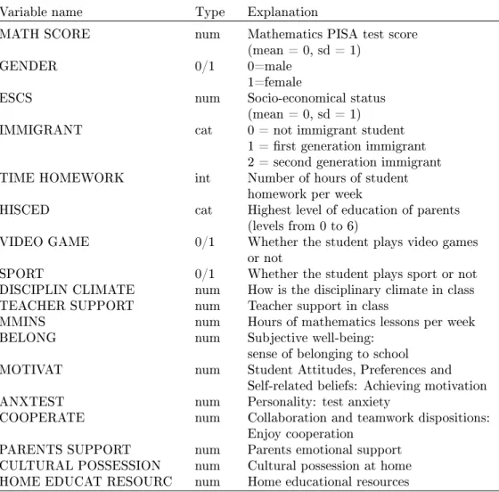
Variable name Type Explanation
MATH SCORE num Mathematics PISA test score (mean = 0, sd = 1)
GENDER 0/1 0=male
1=female
ESCS num Socio-economical status (mean = 0, sd = 1) IMMIGRANT cat 0 = not immigrant student
1 = rst generation immigrant 2 = second generation immigrant TIME HOMEWORK int Number of hours of student
homework per week
HISCED cat Highest level of education of parents (levels from 0 to 6)
VIDEO GAME 0/1 Whether the student plays video games or not
SPORT 0/1 Whether the student plays sport or not DISCIPLIN CLIMATE num How is the disciplinary climate in class TEACHER SUPPORT num Teacher support in class
MMINS num Hours of mathematics lessons per week BELONG num Subjective well-being:
sense of belonging to school MOTIVAT num Student Attitudes, Preferences and
Self-related beliefs: Achieving motivation ANXTEST num Personality: test anxiety
COOPERATE num Collaboration and teamwork dispositions: Enjoy cooperation
PARENTS SUPPORT num Parents emotional support CULTURAL POSSESSION num Cultural possession at home HOME EDUCAT RESOURC num Home educational resources
Table 1: List of student level variables of PISA2015 survey used in the analysis, with the relative explanations. Note: we report here only the test score in mathematics that we use as answer variable in the rst stage of the analysis. In each country, we standardize the test score in order to have mean = 0 and sd = 1. All variables from DISCIPLIN CLIMATE to the end are indicators built by PISA and have mean = 0 and sd = 1.
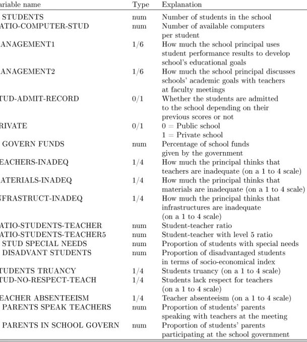
Variable name Type Explanation
#STUDENTS num Number of students in the school
RATIO-COMPUTER-STUD num Number of available computers per student
MANAGEMENT1 1/6 How much the school principal uses student performance results to develop school's educational goals
MANAGEMENT2 1/6 How much the school principal discusses schools' academic goals with teachers at faculty meetings
STUD-ADMIT-RECORD 0/1 Whether the students are admitted to the school depending on their previous scores or not
PRIVATE 0/1 0 = Public school 1 = Private school
%GOVERN FUNDS num Percentage of school funds
given by the government
TEACHERS-INADEQ 1/4 How much the principal thinks that teachers are inadequate (on a 1 to 4 scale) MATERIALS-INADEQ 1/4 How much the principal thinks that
materials are inadequate (on a 1 to 4 scale) INFRASTRUCT-INADEQ 1/4 How much the principal thinks that
infrastructures are inadequate (on a 1 to 4 scale)
RATIO-STUDENTS-TEACHER num Student-teacher ratio
RATIO-STUDENTS-TEACHER5 num Student-teacher with level 5 ratio
%STUD SPECIAL NEEDS num Proportion of students with special needs %DISADVANT STUDENTS num Proportion of disadvantaged students
in terms of socio-economical index STUDENTS TRUANCY 1/4 Students truancy (on a 1 to 4 scale) STUD-NO-RESPECT-TEACH 1/4 Students lack respect for teachers
(on a 1 to 4 scale)
TEACHER ABSENTEEISM 1/4 Teacher absenteeism (on a 1 to 4 scale)
%PARENTS SPEAK TEACHERS num Proportion of students' parents
speaking with teachers at the meeting
%PARENTS IN SCHOOL GOVERN num Proportion of students' parents
participating at the school government Table 2: List of school level variables of PISA2015 survey used in the analysis,
with the relative explanations. Note: all variables of typen1/n2assume integer
values ranging fromn1 ton2, with the maximum value corresponding ton2.
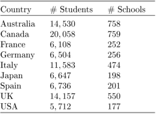
Table 3 reports the sample size in the dierent countries, specifying the num-ber of students and the numnum-ber of schools that participated in the PISA survey.
The sample sizes vary somewhat across countries, but we have chosen the coun-tries used in our analysis so as to ensure that there are sucient observations in each to allow robust conclusions to be drawn.
Lastly, it is worth noting that the percentage of missing data at student level is very low (about 2 to 5%among countries), while at school level it is slightly
higher (about 10 to 25 % among countries). We note, however, that a major
advantage of tree-based algorithms concerns their performance in the presence of missing data - see for example [5] and [18].
Country # Students # Schools
Australia 14,530 758 Canada 20,058 759 France 6,108 252 Germany 6,504 256 Italy 11,583 474 Japan 6,647 198 Spain 6,736 201 UK 14,157 550 USA 5,712 177
Table 3: Sample size in the 9 selected countries.
4 Methodology
We develop and employ a two-stage procedure. In the rst stage, we apply a mixed-eects regression tree (RE-EM tree), with only random intercept, in which we consider two levels of grouping: students (level 1) nested within schools (level 2). The response variable of the mixed-eects model is the student PISA test score in maths, this being regressed against a set of student level characteris-tics (xed coecients), plus a random intercept that describes the school eect. By means of this model, we can both estimate the xed coecients of the stu-dent level predictors on the outcome and the school value-added (corresponding to the random intercept). In the second stage, we regress the estimated school value-added against a set of school level characteristics, by means of regression trees and boosting.
4.1 An introduction to tree-based methods
Given an outcome variable and a set of predictors, tree-based methods for re-gression (see [17]) involve a segmentation or stratication of the predictors space into a number of regions. In order to make a prediction for a given observation, we typically use the mean of the observations in the region to which it belongs. Building a regression tree involves two steps:
1. We divide the predictor space - that is, the set of possible values for
X1, X2. . . , Xp- into J distinct and non-overlapping regions,R1, R2. . . , RJ.
For simplicity, we consider these regions as high-dimensional rectangles (or boxes);
2. For every observation that falls into the region Rj, we make the same
prediction, which is the mean of the response values for the observations inRj.
The regions are chosen in order to minimize the Residual Sum of Squares (RSS): J X j=1 X i∈Rj (yij−yˆRj)2 (1)
whereyˆRj is the mean of the observations within the j-th box andyij is the
i-th observation within the j-th box.
It is useful to contrast this approach with the more conventional methods typically used in the education economics literature - namely a linear functional form imposed on the education production function. In particular, a linear regression model assumes the following functional form:
f(X) =β0+ p X
j=1
Xjβj; (2)
(where p is the number of predictors) whereas regression trees assume a model of the form:
f(X) =
M X
m=1
cmI(X∈Rm) (3)
where M is the total number of distinct regions and R1, . . . , RM represent
the partition of feature space.
Determining which model is more appropriate depends on the problem: if the relationship among the features and the response is well approximated by a linear model, then an approach such as linear regression will likely work well, and will outperform a method such as a regression tree that does not exploit this linear structure (see [40]). If instead there is a highly non-linear and complex relationship between the features and the response, then decision trees may outperform classical approaches. The complex nature of educational production renders this an ideal candidate for exploring the ability of trees-based methods to interrogate non-linearities and interactions in the data.
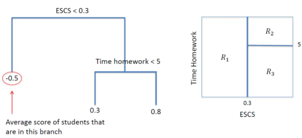
In order to give an example of how to read the result of a regression tree, let us imagine that we want to regress stadardised student test scores (that is a continuous variable with mean = 0 and standard deviation = 1) against three covariates: Economic Social and Cultural Status (ESCS, an indicator of socio-economic status dened to be a continuous variable with mean = 0 and
standard deviation = 1), number of siblings (variable assuming integer values) and time spent on homework (variable assuming integer values) and that Figure 1 reports the result of the regression.
Figure 1: Example of the result of a regression tree. The answer variable is students' tests scores (continuous variable with mean = 0 and sd = 1) and the three covariates are: (i) socioeconomic index (ESCS, continuous variable with mean = 0 and sd = 1), (ii) number of siblings (integer variable) and (iii) time of homework (integer variable counting the hours of homework at home). The image on the left represents the partition of the covariate space into three regions, computed by the regression tree. The image on the right represents the regression tree. Variable number of siblings does not appear in either the two images, since it does not result to be statistically relevant.
First, we notice that the number of siblings does not appear in the tree. This means that this variable is not able to catch any variability in students' test scores and therefore, the tree excludes it from the splits. When reading the tree, every time the condition at the split point is satised, we follow the left branch, otherwise, we follow the one on the right. On the left side of the gure, we see the regression tree while on the right, we see the partition of the covariate space into three regions. The most important variable turns out to be ESCS: a student with an ESCS less than0.3 follows the left branch yielding a
predicted student test score of−0.3; instead, if the student's ESCS exceeds0.3,
he/she goes in the right branch and, at this point, if he/she studies less than 5 hours per week, his/her predicted score is0.3, while if he/she studies more, it
is0.8. The algorithm itself identies the threshold values in order to minimize
the Residual Sum of Squares (RSS). Focusing on the interaction between the two covariates, it is noteworthy that the variable time of homework matters if the ESCS is higher than0.3, while it is irrelevant if the ESCS is lower than0.3.
This brief and simplied explanation serves as a foundation for the methods that we discuss in the following two subsections: RE-EM trees and Boosting,
which are the ones used in the empirical analysis of this paper.
4.2 Multilevel models and RE-EM trees
RE-EM trees (see [36]) work in a similar fashion to random eects (or multilevel) linear models (see [37]) but relax the linearity assumptions of the xed covariates with the response. Given N =PJ
j=1nj individuals, nested within J groups, a
two-level linear model takes the form:
yij =β0+ p X k=1 βkxkij+bj+ij (4) where
i= 1, . . . , N is the index of the i-th individual; j= 1, . . . , J is the index of the j-th group;
yij is the answer variable of the individual i within group j;
βis the (p+1)-dimensional vector of xed coecients; x1ij, . . . , xpij are the p (xed) predictors;
bj is the (random) eect of the group j on the answer variable (value-added
of group j)
andis the vector of the residuals.
Both b and are assumed to be normally distributed with mean 0 and
varianceσ2
b and σ2 respectively. The vector of xed coecientsβ is the same
for all the J groups, while the random interceptbj changes across groups (bj is
the value-added, positive or negative, of the j-th group). The larger isσ2 b the
larger are the dierences across groups.
RE-EM trees merge multilevel models with regression trees, substituting the linear regression of the xed covariates with a regression tree. So, in place of a linear regression, a regression tree is built to model the relationship between the output (test scores) and the inputs (student characteristics). In our case, the individuals are the students and the groups are the schools. If we consider students (level 1) nested within schools (level 2), the two-levels model (with only random intercept), for pupili, i= 1, . . . , nj,n=Pjnj, in schoolj, j= 1, . . . , J
takes the form:
yij =f(xij1, . . . , xijp) +bj+ij (5)
with
b∼N(0, σb2), (6) ∼N(0, σ2) (7)
where f(X) takes the form in (3) and
yij is the maths PISA test score of student i within school j;
xij1, . . . , xijp are the p-predictors at student level;
bj is the random eect of school j, which in this paper is interpreted as a
school-specic value-added (VA) to the educational performance of the student; and
ij is the error.
It is generally assumed that the errors are independent across objects
and are uncorrelated with the eects b. Note, however, that autocorrelation
structure within the errors for a particular object is allowed; to do this, we allow the variance/covariance matrix of errors to be a non-diagonal matrix. The random eectbj is still linear with the outcome, while the xed covariates,
that do not change across groups (schools) are related to the outcome by means of a regression tree.
Moreover, one of the advantages of multilevel models is that we can compute the Proportion of Variability explained by Random Eects (PVRE):
P V RE= σ 2 b σ2 b +σ2 . (8)
PVRE measures how much of the variability of test scores can be attributed to students' characteristics or to structural dierences across schools - in other words, PVRE disentangles the variability of test scores between students from that between schools. Applying RE-EM trees to data of each of the 9 countries, we can both (i) analyse which are the student level variables that are related with students' achievements and in which way and (ii) estimate the school value-added (random eectbj) to students' achievements and compute the proportion
of student scores' variability given by dierences across schools (PVRE). With the aim of adequatly considering the structural dierences between countries, we estimate the educational production function as specied in the equation (5) separately for each country.
4.3 Regression trees and Boosting
Regression trees have a series of advantages: they do not force any functional relationship between the response variable and the covariates; they can be dis-played graphically and are easily interpretable; they can handle qualitative pre-dictors; they allow interactions among the variables and they can handle missing data. Nevertheless, they suer from high variance in the estimation of the rela-tionship between covariates and test scores and they are sensitive to outliers. For these reasons, methods have been developed that serve to reduce variance and increase predictive power; these include bagging, random forests and boosting (see [17]).
Boosting (see [9]) is a method for improving model accuracy, based on the idea that it is easier to nd and average many rough rules of thumb, than to nd a single, highly accurate prediction rule (see [35]). Related techniques
-including bagging, stacking and model averaging - also build and merge results from multiple models, but boosting is unique amongst these in that it is sequen-tial: it is a forward, stagewise procedure. In boosting, models (e.g. regression trees) are tted iteratively to the data, using appropriate methods gradually to increase emphasis on observations that are modelled poorly by the existing collection of trees. Boosting algorithms vary in exactly how they quantify lack of t and select settings for the next iteration. In the context of regression trees and for regression problems, boosting is a form of functional gradient descent. Consider a loss function - in this case, a measure (such as deviance) that repre-sents the loss in predictive performance of the educational production function due to a suboptimal model. Boosting is a numerical optimisation technique for minimising the loss function by adding, at each step, a new tree that is chosen from the available trees on the basis that it most reduces the loss function. In applying the Boosting Regression Tree (BRT) method, the rst regression tree is the one that, for the selected tree size, maximally reduces the loss function. For each subsequent step, the focus is on the residuals: on variation in the re-sponse that is not so far explained by the model. For example, at the second step, a tree is tted to the residuals of the rst tree, and that second tree could contain quite dierent variables and split points compared with the rst. The model is then updated to contain two trees (two terms), and the residuals from this two-term model are calculated, and so on. The process is stagewise (not stepwise), meaning that existing trees are left unchanged as the model is en-larged. The nal BRT model is then a linear combination of many trees (usually hundreds or thousands) that can be thought of as a regression model where each term is a tree. A number of parameters control the model-building process: the learning rate (lr), that drives the velocity with which the tree is learning, that is, it shrinks the contribution of each tree; the maximum number of trees to be considered; the distribution of response variable; and the tree complexity (tc), that is the maximum level of interaction among variables (see [9]).
The increase in predictive power obtained by adopting a BRT approach comes at a cost in terms of ease of interpretation. Indeed, with boosting it is no longer possible to display the tree graphically. But the results can nonetheless be represented quite simply. BRT provides a ranking of the variables, based on their ability to reduce the node purity in the tree (see [4]), that is the signicance of each variable. In order to measure the marginal impact of each predictor, Friedman (see [11]) has proposed the use of partial dependence plots. These plots are based on the following idea: consider an arbitrary model obtained by tting a particular structure (e.g., random forest, support vector machine, or linear regression model) to a given dataset. This dataset includes N observations yk
of a response variabley, fork= 1,2, . . . , N, along withpcovariates denotedxik
fori= 1,2, . . . , p andk= 1,2, . . . , N. The model generates predictions of the
form:
ˆ
yk =F(x1k, x2k, . . . , xpk) (9)
Friedman's partial dependence plots are obtained by computing the following average and plotting it over a useful range ofxvalues:
Φj(x) = 1 N N X k=1 F(x1,k, . . . , xj−1,k, x, xj+1,k, . . . , xp,k) (10)
The idea is that the functionΦj(x)tells us how the value of the variablexj
inuences the model predictionsyˆafter we have averaged out the inuence of
all other variables.
It is possible to visualise also the joint eect of two predictors on the re-sponse variable. The multivariate extension of the partial dependence plots just described is straightforward: the bivariate partial dependence functionΦi,j(x, y)
for two covariatesxi andxj is dened analogously toΦj(x)by averaging over
all other covariates, and this function is still relatively easy to plot and visualise. In particular: Φi,j(x, y) = 1 N N X k=1 F(x1,k, . . . , xi−1,k, x, xi+1,k, . . . , xj−1,k, y, xj+1,k, . . . , xp,k) (11) We therefore apply BRT in each country, in the second stage of our analysis, using the estimated school value-added (rst stage) as response variable and a set of school-level characteristics as predictors.
5 Results
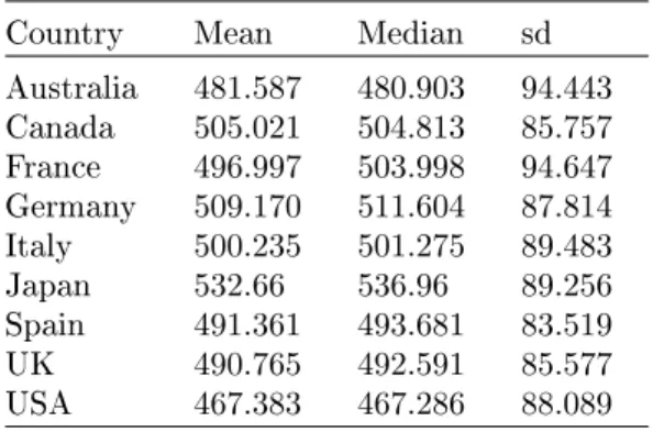
We begin by comparing the results of PISA test in mathematics across the 9
selected countries. Table 4 reports descriptive statistics and Figure 2 shows their distributions.
Country Mean Median sd Australia 481.587 480.903 94.443 Canada 505.021 504.813 85.757 France 496.997 503.998 94.647 Germany 509.170 511.604 87.814 Italy 500.235 501.275 89.483 Japan 532.66 536.96 89.256 Spain 491.361 493.681 83.519 UK 490.765 492.591 85.577 USA 467.383 467.286 88.089
Table 4: Descriptive statistics of students' PISA2015 test scores in mathematics in the 9 selected countries.
Australia Frequency 200 400 600 800 0 500 1000 1500 2000 2500 3000 Canada Frequency 200 400 600 800 0 1000 2000 3000 4000 France Frequency 100 300 500 700 0 200 400 600 800 1000 1200 Germany Frequency 200 300 400 500 600 700 800 0 200 400 600 800 1000 1400 Italy Frequency 200 400 600 800 0 500 1000 1500 2000 2500 Japan Frequency 200 400 600 800 0 200 400 600 800 1000 1400 Spain Frequency 200 300 400 500 600 700 800 0 500 1000 1500 UK Frequency 0 200 400 600 800 0 500 1000 1500 2000 2500 3000 USA Frequency 200 300 400 500 600 700 800 0 200 400 600 800 1000 1200
Figure 2: Histograms of PISA students test scores in mathematics in the 9 selected countries. Red line refers to the mean, green one to the median. Note: by construction, PISA test scores are standardized at the international level for having mean = 500 and standard deviation = 100.
Japan is the country where students, on average, perform higher test scores, followed by Germany, while USA is the country where students report the lowest scores. In almost all the countries, the mean and median are quite close, sug-gesting that the distributions are symmetric; France and Japan are exceptions,
where in both cases the mean is somewhat smaller than the median, suggesting that there is a slightly higher proportion of students with relatively low test scores.
5.1 First stage: Estimating the determinants of students'
test scores and school value-added by using RE-EM
trees
RE-EM trees are tted, separately for each country, using the standardised students' PISA test score in maths as response (in each country students' scores have been standardized, having mean 0 and standard deviation 1) and the entire set of student level variables shown in Table 1 as predictors. A random intercept is given by the grouping factor of students within schools (identied by school ID). Results of this rst stage comprise the regression tree with the coecients for the inputs of individual students' characteristics, the proportion of explained variability by the multilevel model (PV) and the PVRE, within each country.
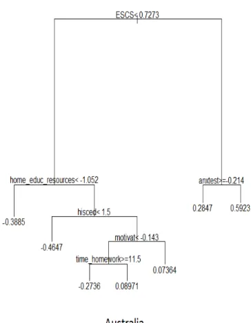
Figure 3 shows the trees of xed student level covariates in each country3,
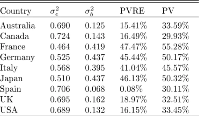
while Table 5 shows the estimated variance of errors, estimated variance of random eects, PV and PVRE of the RE-EM trees models.
3We only report here the gure for Australia, while the gures for other countries are reported in Appendix in Figure 7.
Figure 3: Fixed eect tree of rst stage analysis (RE-EM tree in model 5) in Australia.
Country σ2 σb2 PVRE PV Australia 0.690 0.125 15.41% 33.59% Canada 0.724 0.143 16.49% 29.93% France 0.464 0.419 47.47% 55.28% Germany 0.525 0.437 45.44% 50.17% Italy 0.568 0.395 41.04% 45.57% Japan 0.510 0.437 46.13% 50.32% Spain 0.706 0.068 0.08% 30.11% UK 0.695 0.162 18.97% 32.51% USA 0.689 0.132 16.15% 33.45%
Table 5: RE-EM trees results in the nine selected countries.
The ability of student features to explain students' achievements varies markedly across countries. In some countries, a quite substantial proportion of the dierences in students' achievements are explained by student level vari-ables such as socio-economic index, immigrant status, anxiety in dealing with the scholastic life, self-motivation and so on. France, Japan and Germany, that have high PVs (55.28%,50.32% and50.17% respectively), are examples of this
kind. In other countries, such as Canada and Spain, it seems that these student characteristics are not sucient to explain much of the variability in outcomes. Despite these dierences, Figure 7 in Appendix shows that the impact of several types of student characteristics are coherent across countries. In almost all the countries, the grape of the most important variables includes (1) the indicator that measures students' self-reported anxiety toward tests, (2) socio-economic index (ESCS) and (3) the indicator measuring the self-reported motivation. In particular, the ESCS turns out to be the most important variable within ve countries out of the nine (Australia, France, Spain, UK and USA). In Canada, Germany and Italy, the most signicant variable is ANXTEST: students that feel anxious in their studies have on average lower test scores than more con-dent stucon-dents. Japan is the only country where stucon-dents' self-motivation is the most important variable: if a student has an index of self-motivation less than a certain threshold (in this case, less than −0.9017), then no other variables
matter in predicting achievement; otherwise, parents' education and anxiety matter. Other recurrent variables are the highest educational level of parents (HISCED), the educational resources at home, the disciplinary climate and the number of minutes in the maths lesson. Parental education is a particularly rel-evant variable in Australia, Italy and Japan. Higher levels of parental education are associated with better student achievement. While in Australia and Italy, the dierent impact of parental education is between parents with less or more than ISCED2 (lower secondary), in Japan the dierence is between students with parents with less or more than ISCED4 (post-secondary). Disciplinary climate results to be an important factor in UK and USA: apparently, students that perceive a good disciplinary climate in the class, perform on average better
than others.
When tuning to the estimation of school value-added, it diers across coun-tries, with some countries showing a stronger role of schools in aecting test scores than others. In France, for example, almost the 50% (PVRE =47.47%)
of the unexplained variability among students is captured by the school eect. This means that results of students attending dierent schools also dier, prob-ably due to heterogeneity in schools' quality. By way of contrast, Spain is a country in which students' achievements are quite homogeneous across schools (PVRE = 0.08%). In general, schools have a clear role to play in explaining
the variability of students' scores in France, Japan, Germany and Italy (about
40/45%); in Australia, Canada, UK and the USA, a smaller - but still
non-negligible - portion of variability is explained at school level (about15/20%).
This is a nding with very clear policy implications - policies aimed at schools (rather than, say, families) are likely to have much more potency in the former group of countries than in the latter.
Dierent students' achievements across schools may be the consequence of dierent school policy and teaching programmes or of the socio-economic com-position of the school body (see [25]). While the available data and the proposed methodology do not allow investigation of the channels that drive the causal re-lationships between schools' characteristics and test scores, the next section uses regression trees and boosting to show correlations between schools' features and their estimated value-added.
5.2 Second stage: Modelling the determinants of school
value-added through regression trees and boosting
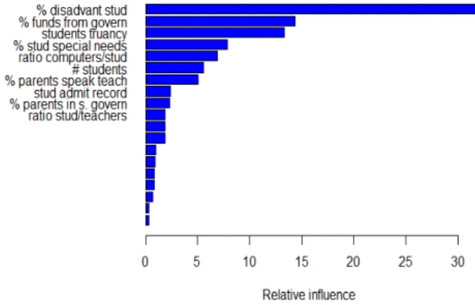
In the second stage of the analysis, we run, within each country, a regression model based on trees and boosting. The response variable is the school value-added, as estimated at the rst stage, while the predictors are the school level variables described in previous section and contained in the questionnaire lled by school principals. Figure 4 and Table 6 show the variable importance ranking within each country4 and the proportion of total variability explained by the
model, respectively.
4We only report here the gure for Australia, while the gures for other countries are reported in Appendix in Figure 8.
Figure 4: School level variables importance ranking in the second stage of the analysis in Australia. Boosting creates a ranking of the relative inuences of the covariates on the outcome variable (school value-added). To lighten the reading, we report here only the rst ten most important variables (where the most important variable is the one able to catch the bigger part of variability in the outcome).
Australia Canada France Germany Italy PV 40.36% 28.09% 59.13% 53.08% 28.09%
Japan Spain UK USA PV 30.87% 14.15% 39.12% 35.81%
Table 6: Proportion of explained variability (PV) of the second stage boosting model, in the 9 selected countries.
We report in the gures only the ten most important variables within each country, both because the remaining variables are statistically irrelevant and to lighten the reading. School size (#students), proportion of disadvantaged
students, proportion of students with special needs, students' truancy and the ratio of computers to students are typically the most important variables in each country (see Figure 8 in Appendix). This means that the school value-added is mainly associated with students' socioeconomic composition and to school size, more so than with managerial characteristics or proxies for resources, as inadequacy of materials and infrastructure. Besides these four main variables, participation of parents, measured both as proportion of parents speaking with
teachers and participating in school governance, and the percentage of funds given by the government are also important in some countries to qualify the estimated schools' value-added.
5.2.1 Describing the patterns of the impact of school variables on schools' value-added
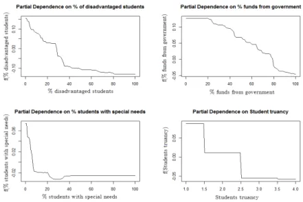
After identifying the important variables, in order to detect the magnitude and the way in which these predictors are associated with the response, we visualise in Figure 5 the partial plots of the four most signicant variables within each country5, noting that these dier across countries.
Figure 5: Partial plot of the four most important school level variables in the association with school value-added, in Australia. Note: the selection of the four most signicant variables is taken from Figure 4 and the explanation of each school level covariate is given in Table 2.
The proportion of disadvantaged students is one of the four most important variables in all the countries except for Japan. Schools with higher proportions of disadvantaged students are those with lower estimated value-added. On aver-age, schools with a high proportion of disadvantaged students suer a negative impact on performances. In particular, in almost all countries, the impact of this variable on schools' value-added is negative in its range from0%to30/40%.
5We only report here the gure for Australia, while the gures for other countries are reported in Appendix in Figure 9.
By way of contrast, in the USA, schools in which the proportion of disadvan-taged students lies between 0 and 20 tend not to dier in terms of outcomes
ceteris paribus, while there is a monotonic negative association between the co-variate and the response in the coco-variate range between20and100. Thus, there
are countries in which the substantial dierence is between schools composed by only advantaged students and schools with a minimum proportion of dis-advantaged ones, while there are countries, such as the USA, in which the the proportion of disadvantaged students is inuential only if it is quite high (more than20%).
Another important determinant of outcomes in all countries, with the excep-tion of Australia, is school size. In general, bigger schools are associated with higher school value-added. The impact of this variable is highly nonlinear and this can be an explanation about why some previous literature fails to nd any statistical (linear) correlation between performances and size. In all countries, except for Australia and USA, the school value-added rapidly increases when the school size ranges between about 500 and1,000 students. Schools smaller
than500 students perform in a quite similar way to schools larger than about 1,000students. The USA provides an interesting exception: very small schools
(with fewer than500students) are associated with very high school value-added,
while there is a negative peak corresponding to schools attended by about500
students, that is the value associated with the lowest school value-added. Again, from500on, larger schools are estimated to have higher value-added.
The proportion of students with special needs is important as a determinant of outcomes in all countries, except Canada and Japan. Schools with a higher proportion of students with special needs are associated to lower school value-added. Again, there is a gap in the response value when the covariate ranges between0%and20%. The number of schools with more than20%of students
with special needs is small, but still we have observations in this range that do not dier in their impact on the response.
Another recurrent important variable is the one measuring the students tru-ancy. Students truancy is an indicator about how much students take seriously their presence at school and therefore, their education. In Australia, Canada, Japan and USA it is one of the four most important variables. Schools with higher proportion of students that tend to skip school days are associated to lower school value-added, in a quite intuitive way, with strong eects after a threshold when the number of days skipped is>2.5.
The percentage of funds given to the school from the government is a key determinant of schools' eectiveness in both Australia and Japan. In Aus-tralia, the trend is very well dened: when the percentage of funds given by the government increases, the school value-added decreases. From the literature (see [20] and [2]), we know that in Australia, private schools, which receive less funds from the government respect to public schools, are more likely to perform better than public ones and therefore these two aspects are probably strongly connected. Even if a dummy variable for public/private schools is considered, the percentage of funds given by the government still reects some of the pub-lic/private heterogeneities and it is actually able to catch more variability in
the response than the dummy variable. Also in Japan the partial eect of the percentage of funds given by the government on the school value-added is re-lated to the dierence between private and public schools. In Japan, contrary to Australia, PISA2015 data indicate that private schools have, on average, lower performance when compared with public schools. Moreover, private schools usu-ally receive about40/50%of their funds from the government. The trend of the
impact of the covariate on the response is less clear than the one in Australia. Lastly, in Canada and in Italy the percentage of parents speaking with teach-ers or participating in school governance are important. An increase in cofactor values is positively associated with the school value-added: schools in which parents are actively interested in their children's education experience more favourable outcomes than do others. Likewise, in Spain the percentage of par-ents participating in school governance, when in the range from 0 to 50%, has
a positive eect on outcomes.
The last variable that appears in the four most important variables of France, Germany, Japan and UK is the number of computers per student (ratio comp / stud). This covariate has a counterintuitive association with school value-added. In Japan and UK (see Japan and UK panels in Figure 9 in Appendix), an increase of number of computers per student is associated with a decrease in school value-added. In Germany (see Germany panel in Figure 9 in Appendix), there is a peak around 0.4 and a trough around 0.6. Lastly, in France (see
France panel in Figure 9 in Appendix), the highest value-added corresponds to zero computers, but there is a peak around 1, maybe suggesting that one
computer per person is the right balance. A possible interpretation of these trends is that too many computers (more than one per person) may be sign of inecient management of school funds. Alternatively it might be the case that national policies have concentrated the IT facilities in less advantaged schools with lower test scores - in this case, the statistical relationship would be biased. 5.2.2 Describing the impact of joint variables on schools'
value-added
Up to this point, we have investigated the partial eect of predictors one by one, on a ceteris paribus basis. But one of the main strengths of the regression tree approach is that it allows consideration of circumstances in which more than one cofactor changes simultaneously, so aecting simultaneously the dependent variable (in our case, school value-added). We now turn, therefore, to focus on the visualisation of the joint eect of two predictors on the response, and in so doing investigate the interaction eect of the most signicant variables within each country (Figure 6)6. Again, the choice of the variables to be included in the
graphical illustration is based on the variables that, in the dierent countries, turned out to be most important in aecting the estimated schools' value-added.
6We only report here the gure for Australia, while the gures for other countries are reported in Appendix in Figure 10.
Figure 6: Joint partial plot of the most important school level variables in association with school value-added, in Australia. Notes: 1. Colors represent the scale of the values of the response (school value-added). 2. The selection of variables is based on the group of the variables that turn out to be signicant in previous steps.
In several countries, the impact on outcomes of the joint association be-tween the proportion of disadvantaged students and school size is of interest. From Australia and USA panels, we know that in most countries larger schools perform better than smaller ones and schools with a high proportion of disad-vantaged students perform less successfully than others. The extent to which dierences in school size aect outcomes depends critically on how high is the proportion of disadvantaged students, however. In Italy and Spain, the pro-portion of disadvantaged students seems to have a clear negative impact even in the big schools, while small schools with a low proportion of disadvantaged students are not associated with negative eect on value-added. In UK and USA, the interaction is much weaker in the sense that the high proportion of disadvantaged students has a negative impact, almost independently from the school size. The dierence between these two countries is that while in UK the threshold value of proportion of disadvantaged students to have a negative impact on the response is about 20/30%, in the USA is much higher, around 70/80%.
Interaction between two variables about the students' socioeconomic compo-sition - namely the proportion of socioeconomically disadvantaged students and proportion of students with special needs - is also interesting and instructive. In France, schools in which both percentages are low perform better than the average while schools where both percentages are high perform worse. However, schools with a high proportion of disadvantaged students nevertheless manage average performance if they have a very small proportion of students with spe-cial needs (and vice versa). In Germany and Italy, schools with a low proportion
of disadvantaged students perform better than the average and the increasing proportion of students with special needs does not aect this performance. On the contrary, schools with a high proportion of disadvantaged students perform worse than the average and the increasing proportion of students with special needs worsens the results even more. In UK, the increase in both proportions contributes to lower school value-added in an almost symmetric way.
Truancy is another variable whose interaction with school size and school body composition is worthy of investigation. Truancy is dened by OECD as the propensity for students to skip classes without justication. In Japan, truancy is associated with very low school value-added only when considering small schools, while, even if it has again a negative impact, we still have positive school value-added in big schools with high students truancy. In USA, schools with low levels of truancy perform better than the average while schools with high truancy rates perform worse than the average, but there is an important interaction with school size - truancy has a more negative association to test scores in smaller rather than in larger schools. In Australia and in Canada, the interaction between students truancy and proportion of disadvantaged students is similar: schools with both high (low) truancy and high (low) proportion of dis-advantaged students are associated with negative (positive) school value-added. But, schools with high truancy rates and a low proportion of disadvantaged students (and vice versa), are still able to achieve average performance.
In Australia and Japan, truancy and percentage of funds given by the gov-ernment are very important variables but they interact in an heterogeneous way to aect schools' performance. In Australia, schools with both high (low) students truancy and high (low) percentage of funds given by the government are associated with negative (positive) eects on school value-added, but, in all the other cases, this relationship doen not hold. Instead in Japan, schools with low (high) students truancy perform worse (better) than the average, almost independently from the percentage of funds given by the government.
The last interaction that deserves attention is the one between school size and percentage of parents participating in school governance in Spain: the size of the school is associated with positive school value-added, but only if par-ents actively participate at the school government and are interested in their children's education.
The visualization of joint partial plots to characterise the determinants of schools' value-added proves to be a powerful tool for analysts and decision mak-ers. Indeed, these gures provide an immediate sense of which are the variables with more or less inuence on schools' value-added, while simultaneously pro-viding information covering the whole distribution of the impacting variables, without forcing to concentrate on average correlations.
6 Discussion, concluding remarks and policy
im-plications
The availability of large scale datasets allowing comparative analysis of edu-cational performance has been a major boost to researchers interested in the educational production function. In this paper, we have applied new methods of analysis, drawn from the machine learning literature, to examine the deter-minants of students' test scores and schools' value-added. The results conrm many of the relationships we knew already from statistical analysis, but provide a new and enriched understanding of how both nonlinearities amongst and in-teractions between cofactors determine educational performance. These insights come from a recognition that the education process is complex, unknown in its specic mechanisms and heterogeneous across countries. The tree-based meth-ods that we use represent an inductive and non deductive way to explain the associations among variables, having two main advantages respect to the classi-cal statisticlassi-cal methods: they do not force any functional relationships between the response (students' results) and the covariates (students' characteristics) and they allow for interactions among the variables.
The rst stage of our analysis shows that student-level variables are able to explain part of the variability in their achievements: socio-economic index, anxiety, motivation, gender, and parental education are some of the most inu-ential variables. Their association to test scores and their ability in explaining variability in students' achievements are dier substantially across countries. The percentage of variability in students' achievements explained at school level (schools' value-added in our terminology here) also varies across coun-tries. Those countries in which the estimated variance of schools' value-added is high are characterised by heterogeneity at school level. On the contrary, coun-tries where the variance of schools' value-added is limited in magnitude oer a more homogeneous experience across schools. There are clear policy impli-cations in noting, for example, that the ratio of students to teachers has high relative inuence in Canada, Japan and Spain, but not elsewhere. In many countries, the actions that can most eectively improve educational outcomes are not educational policies per se, but rather social policies.
After estimating the school value-added in the rst stage, we correlate it to school level characteristics in the second stage. Again, we nd dierent school level variables associated to school value-added across countries. The main focus in this stage is the eect of interactions between cofactors, which is modelled by means of joint partial plots. As we have seen, the impact on performance of changes in one variable often depends crucially on the value of other explanatory variables.
Tree-based methods complement linear regression models of educational per-formance by augmenting them with a richer interrogation of the data. The impact of student and school level variables are often not simply linearly asso-ciated with students' achievements; we have uncovered evidence in the data of considerably more complex (and intuitively plausible) patterns. The strength
of the machine learning method, in this perspective, is that they literally "learn from the data", nding the dominant patterns without any assumption. Armed with the rened understanding of how dierent policies can impact dierently on schools in various circumstances, policy-makers can better implement change aimed at improved performance.
Several policy implications can be drawn from our analysis. The results show the relationship between test scores and both school and individual factors to be quite complex, and this presents a challenge to naïve interpretations of school performance tables. A particularly salient aspect of this complexity relates to dierences across countries in the impact on educational performance of vari-ables that are not usually thought to pertain to educational policy. Notably in several countries in this study (but not in others), the rst branch of the regression tree is dened by ESCS - indicating that (in these countries, but not elsewhere) issues in the sphere of education might most eectively be addressed using social rather than educational policies. The machine learning tools used thus highlight in sharp relief some issues with high policy relevance.
The results obtained in the present paper should be viewed alongside other research drawn from the literature on educational production functions. In common with much contemporary applied economic research, these studies place emphasis on causality. Further research is needed to introduce sophisticated analysis of causality in the machine learning context, specically as it applies in the sphere of education.
Acknowledgements
The authors are grateful to Professor Anna Maria Paganoni for the statistical support during the work.