C
HAPTER
2
Sequences and Equivalence
Chapter 2 provides you an opportunity to review and strengthen your algebra skills while you learn about arithmetic and geometric sequences. Early in the chapter, you will find yourself using familiar strategies such as looking for patterns, making tables, and guessing and checking to write algebraic rules describing sequences of numbers. Later in the chapter, you will develop shortcuts for writing rules for certain kinds of sequences.
One purpose of this course is to provide you with multiple opportunities to become comfortable representing real-life situations and relationships with variables and equations. Another purpose is to strengthen your algebraic
manipulation skills. In the second section of this chapter, you will focus on rewriting expressions and solving equations.
In this chapter, you will learn how to:
Understand and recognize growth by multiplication and growth by addition. Generate multiple representations of arithmetic and geometric sequences. Understand the connections between sequences and functions.
Represent any term of a sequence with an algebraic expression. Solve equations by first rewriting them in more convenient forms.
Section 2.1 This section begins with lessons that ask you to describe the growth of a rabbit population and the decreasing rebound height of a bouncing ball. You will use tables, graphs, and equations to represent arithmetic and geometric sequences. You will also learn some of the specialized vocabulary used when discussing sequences.
Section 2.2 Here, you will look at the meaning of equivalence. You will develop algebraic strategies for rewriting expressions and equations, creating equivalent equations that you already have the tools to solve.
?
Think about these questions throughout this chapter:
How can I represent it? What are the connections?
How can I rewrite it? What tools can I use?
?
=
Chapter 2 Teacher Guide
Section Lesson Days Lesson Title Materials Homework
2.1.1 2 Representing
Exponential Growth
• Lesson 1.1.2A Res. Pg.
(optional) • Transparencies and overhead pens • Overhead graphing calculator 2-6 to 2-12 and 2-13 to 2-19 2.1.2 1 Rebound Ratios • Bouncy balls
• Meter sticks or longer measuring devices
• Lesson 1.1.2A Res. Pg.
(optional)
• Overhead graphing
calculator (optional)
2-24 to 2-29
2.1.3 1 The Bouncing Ball and
Exponential Decay
• Bouncy balls
• Meter sticks or longer measuring devices
• Lesson 1.1.2A Res. Pg.
(optional)
2-36 to 2-41
2.1.4 2 Generating and
Investigating Sequences
• Lesson 2.1.4A Res. Pg.
• Lesson 2.1.4B Res. Pg.
• Lesson 2.1.4C Res. Pg.
• Scissors
• Tape, stapler, or glue
• Markers or colored pencils 2-46 to 2-52 and 2-53 to 2-60 2.1.5 1 Generalizing Arithmetic Sequences None 2-71 to 2-77 2.1.6 1 Using Multipliers to Solve Problems • Crayons or colored
pencils (for use on an optional problem)
2-86 to 2-91
2.1.7 1 Comparing Sequences
and Functions None 2-98 to 2-105
2.1
2.1.8 1 Sequences that Begin
with n = 1
• Lesson 2.1.8 Res. Pg.
• Transparencies and
overhead pens
2-110 to 2-117
2.2.1 1 Equivalent Expressions None 2-122 to 2-129
2.2.2 1 Area Models and
Equivalent Expressions None 2-135 to 2-142
2.2
2.2.3 1 Solving by Rewriting • Lesson 2.2.3 Res. Pg.
(optional) 2-149 to 2-156
Suggested Assessment Plan for Chapter 2
For complete discussion and recommendations about assessment strategies and grading, refer to the “Assessment” section of this teacher edition.
Participation Quiz Student
Presentations Portfolios/ Growth Samples
Lesson 2.1.3
As teams sort sequences multiple times, use the Participation Quiz to highlight team behaviors that encourage students to share multiple ways of seeing sequences. You can also reinforce the role of the Task Manager by making sure that all team members understand and agree before moving on.
Lesson 2.2.1 or 2.2.3
Students presenting equivalent expressions in problem 2-120 or expressions for the tile pattern in problem 2-148 can help you establish the value of multiple ways of seeing patterns.
Lesson 2.1.1 – Multiplying Like Bunnies
This lesson can provide evidence in a portfolio of students’ beginning understanding of exponential growth. Future work will allow students multiple opportunities to show growth over time.
Closure: Growth Over Time
Students can showcase their early
understanding of an exponential function. Be sure that they keep this for future comparison. Ideas for Individual Test
In Section 2.1, students learn about arithmetic and geometric sequences. This section offers students a chance to review their understanding of linear relationships and serves as an introduction to exponential functions. To facilitate the connection to linear and exponential functions, throughout the section students will call the first term in the sequence the “initial value” or “term number zero.” It is not until the end of the section that they switch to writing rules with the assumption that the first term is named “term number one.” As you create an individual test, remember not to expect mastery of the new topics yet. Wait to assess students’ abilities to write exponential functions formally until after Chapter 3, when they have had more time to practice in homework and in new contexts. Also, allow time for students to adjust to starting sequences with term number one.
In Section 2.2, students learn about equivalence. This is an early piece in their continuing development of algebraic manipulation skills. At this point, students should be able to determine if two expressions are equivalent by testing values and, in some cases, by simplifying or rewriting those expressions. Many students have a hard time simplifying expressions or solving equations that contain fractions or rational expressions. Do not expect mastery at this time. Wait to assess these skills formally until after Chapter 5, when students will have had a chance to practice in homework and revisit solving strategies with their teams.
More than half of each test should be made up of spiraled material from previous chapters. By the end of this chapter is an appropriate time to test students’ ability to:
• Extend, graph, and write a rule for an arithmetic or geometric sequence, as in problems 2-6, 2-24, 2-39, 2-46, 2-73, 2-100, 2-104, 2-111, 2-128, and 2-153.
• Determine whether a given value is part of an arithmetic sequence, as in problem 2-71.
• Determine if two expressions or equations are equivalent, as in problems 2-125, 2-135, and 2-150.
• Create equivalent expressions, as in problem 2-122.
• Multiply polynomials, as in problems 2-76 and 2-142.
• Solve systems of linear equations, as in problems 2-7, 2-25, 2-27, 2-38, 2-47, and 2-101. Ideas for Team Test
Overview of the Chapter
This chapter has five main objectives:
• Students will learn what sequences are and will become familiar with two important types of sequences: arithmetic and geometric.
• Students will write expressions for the nth
term of arithmetic and geometric sequences. • Students will recognize the connections between arithmetic and geometric sequences and
linear and exponential functions.
• Students will enhance their understanding of functions by comparing and contrasting arithmetic and geometric sequences with linear and exponential functions.
• Students will strengthen their algebraic manipulation skills as they focus on rewriting expressions and solving equations by rewriting.
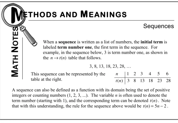
In Lessons 2.1.1 through 2.1.7, n=0 will be used to denote the initial value of a sequence. Although a common approach is to start sequences with n=1, students often find this approach confusing when they try to use sequences to model real-life phenomena. In addition, using n=0 to denote the initial value yields the formula t(n)=a+d!n for the nth
term of an arithmetic sequence, a direct analogy to the general equation of a linear function, f(x)=mx+b. This makes it much more intuitive for students to recognize arithmetic sequences for what they are: linear functions restricted to the domain of whole numbers.
When students start to work with sequences, especially sequences with the measurement of time as the independent variable, you may want to describe the sequence to students as follows:
t(0)=the initial value; t(1)=the value after one hour, day, month, etc.; t(2)=the value after two hours, days, months, etc. To help students understand this approach, the chapter begins with an application in which students can use problem-solving skills to develop a formula for the nth
term of a sequence with initial value n=0. In Lesson 2.1.8, the transition is made to start sequences with n=1.
Teamwork
The lessons in this chapter and throughout the course continue to depend on students working in teams. They do this so that students help and support each other, as well as to expose them to multiple ways of solving problems and seeing mathematical relationships. If you have not changed teams since the beginning of Chapter 1, this is a good time to switch study teams to allow students to learn to work with other students and to be exposed to different ways of seeing the topics they are studying.
If you are using team roles in your class, assign students new roles when they switch teams. Suggestions for doing this are included in Lesson 2.1.1, as well as in the “Using Study Teams for Effective Learning” section in this Teacher Edition. As students transition to new teams, it is important to reiterate your expectations of study teams and remind students of the qualities of successful teams. Providing specific instructions for each role will also be important, as students will be performing new roles. Emphasize the questions, statements, and key words that students can use to fulfill their assigned roles.
Where Is This Going?
Working with arithmetic and geometric sequences allows students to review their Algebra 1 skills in a new context. The work with geometric sequences prepares them for thinking about exponential functions in Chapter 3. By the end of Section 2.1, students will be able to write an expression for the nth
term of an arithmetic or geometric sequence. Students will return to investigate sums of sequences as series in Chapter 12.
In Section 2.2, students begin to work explicitly on algebraic manipulation skills. This will continue in Section 3.2, where students will study equations of lines and exponential functions through two points; in Chapter 4, where students will rewrite equations of parabolas in graphing form; and in Chapter 5, the focus of which is primarily solving equations, systems of equations, and inequalities. This focus continues through Chapter 6, where students find and check inverses algebraically, and through Chapter 7, where students learn the properties of logarithms. The remaining chapters require students to use their algebra skills to solve polynomial equations, derive general formulas for conic sections, prove formulas for sums of series, and solve trigonometric identities.
Lesson 2.1.1 How does the pattern grow?
Representing Exponential Growth
Lesson Objective: Students will represent exponential growth with a diagram, table,
equation, and graph. Students will write equations based on the patterns in their tables, recognize patterns of exponential growth, and use their equations to make predictions.
Length of Activity: Two days (approximately 100 minutes)
Core Problems: Problem 2-1, parts (a) and (b) of problem 2-3, and problem 2-4 (along with problem 2-2 if using Further Guidance)
Ways of Thinking: Justifying, generalizing, choosing a strategy
Materials: Lesson 1.1.2A Resource Page (“Team Roles”), one per team (optional) Blank overhead transparencies and overhead pens, one set per team Graphing calculator with display capability
Lesson Overview: This lesson introduces students to exponential growth. On the first day of the lesson, students generate exponential data based on a situation and represent it with diagrams, tables, and equations. Students extend their work on the second day by deciding whether the relationships they explored are linear.
Suggested Lesson Activity:
Day 1: To introduce this lesson, remind students that in Lesson 1.2.2, they began to characterize the family of linear functions in terms of multiple representations. Ask students what other families of functions they have worked with, either in Chapter 1 or in previous courses, and
may bring up the families of parabolas or even hyperbolas. You might end the discussion with a statement such as, “In this chapter, we will continue looking closely at families of functions, which you will use to model situations by learning all about the patterns in the function’s growth, tables, equations, and graphs.”
Problem 2-1, “Multiplying Like Bunnies,” asks students to represent a growing population of bunnies first as a diagram, then in a table, and finally as a rule. Before students delve into the problem too deeply, make sure they correctly interpret how the population is growing. At the same time, it is important for students to try developing their own
organizational strategies so they can successfully build on them. One way to accomplish both of these goals is by using the study-team strategy “Teammates Consult.” (Note: Refer to the “Using Study Teams for Effective Learning” section under the “Introductory Materials” tab at the front of this teacher edition for descriptions of study-team strategies.) Discuss this strategy and its purpose briefly with the class and then have a member from each team read the problem. Remind students that during this time they are only allowed to read and discuss their ideas for organizing and solving the problem, but they may not write anything yet. The purpose of this activity is to get students to think thoroughly about the problem before they start working on it. As the discussions are coming to a close, direct teams to work on the problem while one team member records ideas on a piece of paper in the middle of the workspace. As you circulate, observe the organizational strategies of each team. Give each team a transparency and overhead pens and have teams summarize their work to present briefly to the class. It is not necessary to have all teams report, but carefully choose the teams that do and the order in which you want them to present. Try to select teams in an order that causes the ideas to connect and build on each other. Throughout the reporting, students should ask teams brief questions and comments for clarification instead of waiting until after all of the presentations are completed. At the end of each presentation, you could then ask, “As a class, do we agree that…?” and then make sure that all students understand the problem: that each month, each pair of rabbits has two babies, so in the second month, both the original pair of rabbits and the new pair each have two babies, for a total of eight rabbits. Ask each team to decide which organizational strategy makes it easiest to see what is happening with the population of the rabbits. They do not have to agree on a particular strategy but should choose one that works for their team.
A possible diagram that students may come up with is shown below.
In this example, students chose to shade each pair of rabbits that are
Original number (after 0 months) Number of rabbits after 1 month Number of rabbits after 2 months
four months, the total number of rabbits can be found by using the diagram, but diagrams get big and difficult to follow very quickly. This inherently follows the nature of an exponential function; ideally, students will observe this visually.
After teams share, prompt them to return to work with questions such as, “How else can you represent what the diagram is showing?” and “How can you continue the table without having to draw it?” As you circulate, check to see if teams are starting their tables with the initial number of rabbits, that is, the
number of rabbits after zero months have passed, as shown above. A second option for starting class is to have students read through problem 2-1 and the task statement and then start immediately to work. Teams that are struggling can be directed to problem 2-2 for further guidance. Again, it is important to check with each team early in the lesson to see how the team is representing the way the rabbits are
multiplying. See the “Lesson Overview” section of the teacher notes for Lesson 1.1.2 for more information on the use of the “Further Guidance” structure.
As students consider how to extend the table, there are different patterns they might use and different ways to show those patterns. You could encourage them to add a third column to show the pattern they see developing, as shown in the table above. Encourage students to share what they see. At this time, they may not know what pattern is useful for writing an equation. Students are likely to see the entries in the table as doubling or multiplying by 2.
Circulate and listen to teams’ conversations as they work to find an equation that models the data in their table. Remind students to discuss the patterns that they see in the table, since the patterns may help them determine an equation. When teams seem to be either finished or stuck, collect ideas for the equation (y=2!2x and y=2x+1 are most likely). Ask teams to report how they developed their equations. This discussion provides an opportunity for students to think explicitly about what the possible equation is and why some types of functions are not good possibilities. Ask questions such as, “Is this equation linear? How can you tell? How is this new equation related to the patterns in the table?” If teams report more than one form of the equation (such as the two above), you can ask questions such as, “Do both equations work? How can you tell?” and “Are these two equations substantially different, or are they equivalent? How can we tell?” When the class has agreed on
Month # # of Rabbits Patterns 0
1
2
2 8
keep careful track of their work as they leave so they do not lose any ideas in the time between class meetings.
Day 2: Students are likely to find writing the equations for the three cases of problem 2-3 challenging. They may make assumptions about the rule based on a pattern they perceive in their results from
problem 2-1. If this happens, ask students to prove that their rule is correct. Notice that the rule does not appear to have a clear connection to the problem statement. For example, Case 3 asks students to consider a pair of rabbits that has four babies each month. Teams may guess that the equation would be y=2!4x. If students take the time to create a diagram and a table, they will find that the rule is, in fact, y=2!3x. Once teams have found the correct rule, ask them to find connections between the rule and the situation. In the case discussed above, students may say that each pair of rabbits one month corresponds to (or turns into) three pairs of rabbits the following month. Thus, each month the
previous month’s total is multiplied by 3, yielding the base of 3. Be sure to allow enough time for students to discuss and show the
connections between their tables and equations in part (c) of problem 2-3. After teams have completed problem 2-3 (i.e., after they have created their own table and equation and have shown connections between them with color, labels, and other tools), bring the class together. Ask one or two teams to present their tables and equations and ask this question again: “How can we connect the new equation to the patterns in the table?” Students will return to this question in problem 2-5, so collecting initial ideas here is sufficient.
Use problem 2-4 to bring together ideas from this lesson as a class and to help students begin to get a sense of what the graphs of exponential functions look like. Discuss part (a) as a class. Then, using a graphing calculator with display capability, enter the four equations from
problem 2-1 and part (a) of problem 2-3 into the calculator. When all graphs are clearly visible and the window is adjusted to show the graphs clearly, remind students to sketch these graphs on their own papers. Based on their results from problems 2-1 and 2-3, teams should be ready to conclude that these relationships are neither linear nor quadratic. They should also be ready to justify this conclusion using multiple
representations. At this time, it is not necessary for students to see the equation y=abx or to talk formally about exponential functions, as there will be plenty of opportunities to do this later in the chapter. However, after students conclude that these functions are neither linear nor quadratic, it is appropriate to introduce the term exponential function to describe the new kind of equation they have been writing.
Suggested Study Team Collaboration Strategy: For problem 2-1, Teammates Consult
(10 minutes) example, students initially explain that the data for “Multiplying Like Bunnies” is not linear by referring to the table, you can ask, “How would you justify your idea using the graph? How can you justify your idea using the equation?”
The Learning Log entry in problem 2-5 allows students to summarize what they have learned about the kind of pattern they have modeled and generalized. Because students will continue to build an understanding of the patterns and connections among different representations of
exponential functions, it is not necessary for them to have an exhaustive definition or explanation in their Learning Logs at this point.
Team Roles: The tasks in this lesson require study teams to discuss strategies for organizing information both in diagrams and in tables. Facilitators are responsible for making sure that the team members are hearing ideas from all other members of the team and also ensuring that team members are sticking together. Recorder/Reporters should make sure that work is placed in the middle of the workspace so that it is visible to each team member, and, if using “Teammates Consult,” they are responsible for recording and reporting the team’s information. As students look for patterns in tables and try to write equations, it will be important for them to use the tables as visual aids to explain their thinking to each other.
Task Managers should listen for team members’ justifying their ideas and should make sure that all team members participate in team and whole-class conversations and do not talk outside their teams.
Beginning a new chapter is a good opportunity to switch teams and/or team roles. Changing the composition of the teams serves multiple purposes: Students are able to meet and learn to work with other students in the room, which promotes a sense of class community; any difficult interpersonal dynamics that may have developed in a particular team will be reduced; students are able to learn different team roles; students are able to learn how other students in the class think and are thus exposed to different ways of seeing mathematics; and students are less likely to get stuck in their patterns of interaction. Teams can be assigned randomly, by handing out playing cards as students enter the room, by redistributing name cards in a seating chart posted in the room, etc.
If students are working in new teams or are assuming new roles in this lesson, it will be beneficial to review the study-team expectations included in Chapter 1 to remind students of the norms for working together. It is also helpful to use a transparency of the Lesson 1.1.2A Resource Page to introduce role responsibilities to students who assume a new role for the first time. Assign one of the roles the responsibility for making sure that students introduce themselves to their new teams.
2.1.1
How does the pattern grow?
• • • • • • • • • • • • • • • • • • • • • • • • • • • • • • • • • • • • • • • • • • • • • • • • • • • • • • • • • • • • • • • • •
Representing Exponential Growth
Student pages for this lesson are 53 – 59.
In the last chapter, you began to describe families of functions using multiple representations (especially x!y tables, graphs, and equations). In this chapter, you will learn about a new family of functions and the type of growth it models.
2-1. MULTIPLYING LIKE BUNNIES In the book Of Mice and Men by John Steinbeck, two good friends named Lenny and George dream of raising rabbits and living off the land. What if their dream came true?
Suppose Lenny and George started with two rabbits that had two babies after one month, and suppose that every month thereafter, each pair of rabbits had two babies.
Your task: With your team, determine how many rabbits Lenny and George would have after one year. Represent this situation with a diagram, table, and rule. What patterns can you find and how can you generalize them? [ They would have 8192 rabbits after one year. If x represents the number of months that has passed and
y represents the number of bunnies, y=2 · 2x or y=2x+1. ]
What strategies could help us keep track of the total number of rabbits? What patterns can we see in the growth of the rabbit population?
How can we use those patterns to write an equation? How can we predict the total number of rabbits after many
2-2. How can you determine the number of rabbits that will exist at the end of one year? Consider this as you answer the questions below. [ a: Diagrams vary; at the end of one month, there are four rabbits (the original two and their two offspring), so there will be 16 rabbits after three months; b: y=2!·!2x or y=2x+1. ]
a. Draw a diagram to represent how the total number of rabbits is growing each month. How many rabbits will Lenny and George have after three months? b. As the number of rabbits becomes larger, a diagram becomes too cumbersome
to be useful. A table might work better. Organize your information in a table showing the total number of rabbits for the first several months (at least 6 months). What patterns can you find in your table? Use those patterns to write a rule for the relationship between the total number of rabbits and the number of months that have passed since Lenny and George obtained the first pair of rabbits.
2-3. Lenny and George want to raise as many rabbits as possible, so they have a few options to consider. They could start with a larger number of rabbits, or they could raise a breed of rabbits that reproduces faster. How would each of these options change the pattern of growth you observed in the previous problem? Which situation would yield the largest rabbit population after one year? [ a: Case 2: y=10!·!2x,
Case 3: y=2!·!3x, Case 4: y=2!·!4x; b: Case 4 will result in the most rabbits at
the end of one year; c: Answers vary. ]
a. To help answer these questions, model each case below with a table. Then use the patterns in each table to write a rule for each case.
Case 2: Start with 10 rabbits; each pair has 2 babies per month. Case 3: Start with 2 rabbits; each pair has 4 babies per month. Case 4: Start with 2 rabbits; each pair has 6 babies per month.
b. Which case would give Lenny and George the most rabbits after one year?
Justify your answer using a table or rule from part (a).
c. Now make up your own case, stating the initial number of rabbits and the number of babies each pair has per month. Organize your information in a table and write a rule from the pattern you observe in your table. Show how your table is connected to its equation using color-coding, arrows, and any other tools
Further Guidance section ends here.
2-4. A NEW FAMILY?
Is the data in “Multiplying Like Bunnies” linear, or is it an example of some other relationship? [ a: A typical response is that they all change by multiplying by a constant; b: graph shown below right, but descriptions vary; c: It is a new family of functions, and students will learn what to call them in problem 2-5. ]
a. Look back at the x!y tables you created in problem 2-3. What do they all have in common?
b. Graph all four of the equations from problems 2-1 and 2-3 on your graphing calculator. Adjust the viewing window so that all four graphs show up clearly. Then, on paper, sketch the graphs and label each graph with its equation. How would you describe the graphs?
c. Now decide whether the data in the rabbit problem is linear.
Justify your conclusion.
2-5. LEARNING LOG
To represent the growth in number of rabbits in problems 2-1 and 2-3, you discovered a new family of functions that are not linear. Functions in this new family are called
exponential functions. Throughout this chapter and the next, you will learn more about this special family of functions.
Write a Learning Log entry to record what you have learned so far about exponential functions. For example, what do their graphs look like? What patterns do you observe in their tables? Title this entry “Exponential Functions, Part 1” and include today’s date.
y
To solve a system of equations algebraically, it is helpful to reduce the system to a single equation with one variable. One way to do this is by
substitution.
Consider the system at right.
First, look for the equation that is easiest to solve for x or y. In this case, the second equation will be solved for x. Be sure you understand each step in the solution shown at right.
Now replace the x in the other equation
with (!2!2y). This is the substitution step. Notice that this creates a new equivalent equation that has only one variable.
Next, solve for y. Then find x by substituting the value of y (in this case, 0.5) into either original equation and solve for x.
In this example, the solution is x=!3 and y=0.5.
This solution can also be written (–3, 0.5).
Note that you could have solved for x in the other equation or for y in the original equation, and then followed the same process.
M
AT
H
N
O
T
E
S
ETHODS AND
M
EANINGS
Solving Systems, Part I: Substitution
10y!3x=14 2x+4y=!4 2x+4y=!4 2x=!4!4y x=!2!2y 2x+4(0.5)=!4 2x+2=!4 2x=!6 x=!3 10y!3(!2!2y)=14 10y+6+6y=14 16y+6=14 16y=8 y=0.5
2-6. What if the data for Lenny and George (from problem 2-1) matched the data in each table below? Assuming that the growth of the rabbits multiplies as it did in
problem 2-1, complete each of the following tables. Show your thinking or give a brief explanation of how you know what the missing entries are. [ a: 108, 324; b: 12, 48 ]
a. b.
2-7. Solve the following systems of equations algebraically. Then graph each system to confirm your solution. If you need help, refer to the Math Notes box in Lesson 2.1.1.
[ a: (1, 2), b: (–3, 2) ]
a. x+y= 3 x=3y!5
b. x!y=!5 y=!2x!4
2-8. For the function f(x)= 2x!6 3, find the value of each expression below. [ a: –6, b: –2, c: ! 2
3, d: undefined, e: x=2.25 ]
a. f(1) b. f(0) c. f(!3) d. f(1.5) e. What value of x would make f(x)=4?
2-9. Benjamin is taking Algebra 1 and is stuck on the problem shown below. Examine his work so far and help him by showing and explaining the remaining steps. [ 27a6b3 ]
Original problem: Simplify (3a2b)3.
He knows that (3a2b)3=(3a2b)(3a2b)(3a2b). Now what?
Months Rabbits 0 4 1 12 2 36 3 4 Months Rabbits 0 6 1 2 24 3 4 96
2-10. Simplify each expression below. Be sure to show your work. (Hint: Use your understanding of the meaning of exponents to expand each expression and then simplify.) Assume that the denominators in parts (b) and (c) are not equal to zero.
[ a: x5, b: y3, c: 1 x4 , d: x 6 ] a. (x3)(x2) b. y5 y2 c. x3 x7 d. (x 2)3
2-11. The equation of a line describes the relationship between the x- and y-coordinates of the points on the line. [ a: Sample answers: (3, 0)and(3, 1); All points on this line have 3 as an x-coordinate. x=3, b: y=!1, c: x = 0 ]
a. Plot the points (3,!!1), (3,!2), and (3,!4) and draw the line that passes through them. State the coordinates of two more points on the line. Then answer this question: What will be true of the coordinates of any other point on this line? Now write an equation that says exactly the same thing. (Do not worry if it is very simple! If it accurately describes all the points on this line, it is correct.) b. Plot the points (5,!!1), (1,!!1), and (!3,!!1). What is the equation of the line
that goes through these points?
c. Choose any three points on the y-axis. What must be the equation of the line that goes through those points?
2-12. Carmel wants to become a “Fraction Master.” He has come to you for instruction.
[ a: Find a common denominator (36), convert each fraction to 36ths
, subtract, simplifies to ! 1
36; b: Find a common denominator (2xy), convert each
fraction, 3y
2xy+ 2xy8 = 3y+8
2xy . ]
a. Help Carmel by demonstrating and explaining every step necessary to simplify the problem at right.
b. “Oh no!” exclaimed Carmel. “This one is hard!” Show him every step he needs to simplify the problem at right. (Note that from this point on in the course, you may assume that all values of a variable that would make a denominator zero are excluded.)
2-13. Jill is studying a strange bacterium. When she first looks at the bacteria, there are 1000 cells in her sample. The next day, there are 2000 cells. Intrigued, she comes back the next day to find that there are 4000 cells! Create multiple representations (table, graph, and rule) of the function. The inputs are the days that have passed after
2 9 ! 1 4 3 2x+ 4 xy
2-14. Write each expression below in a simpler form. [ a: 52 = 25, b: 351, c: 3!44 7 , d: 6104 ] a. 5723 5721 b. 3300 3249 c. 3!41001 7!4997 d. (654 )11 (649 )10
2-15. Jackie and Alexandra were working on homework together when Jackie said, “I got x=5 as the solution, but it looks like you got something different. Which solution is right?”
“I think you made a mistake,” said Alexa. Did Jackie make a mistake? Help Jackie figure out whether she made a mistake and,
if she did, explain her mistake and show her how to solve the equation correctly. Jackie’s work is shown above right. [ Jackie squared the binomials incorrectly. It should be: x2 +8x+16!2x!5=x2 !2x+1, 6x+11=!2x+1, 8x=!10, and
x=!1.25. ]
2-16. Solve each of the following equations. [ a: m = 5, b: a =4!7 "1.80 ]
a. m6!=!1518 b. !7!=!a4
2-17. Write the equation of each line described below. [ a: y=!2x+7, b: y=!3
2x+6 ] a. A line with slope –2 and y-intercept 7.
b. A line with slope –23and x-intercept (4,!0).
2-18. Perform each operation in part (a) through (d) below. [ a: 7m
12 , b: 12 , c: 8my x2 , d: 2 5 ] a. m4 + m3 b. 2x! x!12 c. (8mx2)!(mxy ) d. (23)÷(53) (x+4)2!2x!5=(x!1)2 x2+16!2x!5=x2+1 16!2x!5=1 11!2x=1 !2x=!10 x=5
2-19. The dartboard shown at right is in the shape of an equilateral triangle. It has a smaller equilateral triangle in the center, which was made by joining the midpoints of the three edges. If a dart hits the board at random, what is the probability that: [ a: 1
4 , b: 34 ] a. The dart hits the center triangle?
b. The dart misses the center triangle?
Lesson 2.1.2 How high will it bounce?
Rebound Ratios
Lesson Objective: Students will generate data and will model the data with tables, rules, and graphs. They will calculate the rebound ratio when a ball bounces.
Length of Activity: One day (approximately 50 minutes)
Core Problems: Problems 2-20 through 2-23
Ways of Thinking: Justifying, generalizing
Materials: Small, rubber, very bouncy balls, one per team
Meter sticks, two per team (or one longer measuring device per team, as explained in “Materials Preparation” below)
Lesson 1.1.2A Resource Page (“Team Roles”) (optional) Graphing calculator with display capabilities (optional)
Materials Preparation:
To measure the rebound height of a bouncing ball, each team will need a measuring tool set up against a wall. Meter sticks or tape measures work, or you can set up a strip of paper (such as adding machine tape) with one-centimeter increments marked ahead of time. Note that you will need the same materials and setup for Lesson 2.1.3.
Lesson Overview: Students will record and model data comparing the height from which a
ball is dropped and the height to which it rebounds. The data should be linear, and students will determine that the slope of the representative line is the “rebound ratio” of the ball. In the next lesson, students will use this rebound ratio to investigate exponential decay.
Suggested Lesson Activity:
After a brief lesson introduction, give students 5 minutes to respond to problem 2-20. As students share their ideas, be sure that the idea of using the ratio rebound!heightstarting!height to quantify each ball’s “bounciness” comes up. Move teams on to problem 2-21. Give teams a few minutes to discuss the questions in the text and plan their experiment. Teams should call you over when they think have a viable plan. Ask them to describe their
viable, point out to them the ways that you are not sure it will work and give them more time to revise it and call you back again. Note that to get consistent results, teams should measure heights from the floor to the same place on the ball each time. Many students decide that the bottom of the ball makes most sense, since it is the part that touches the floor. When teams have collected data, they should move on to problem 2-22. As they graph their data, they should find a line that fits their data and recognize that its slope represents the ball’s rebound ratio.
As teams work, check their graphs for completeness and accuracy. Make sure students identify the starting height as the independent variable and the rebound height as the dependent variable. Since students do not use a starting height of zero, they may not realize that they should include the point (0, 0) on their graph. Make sure they understand how to interpret the y-intercept as it relates to their task. As you circulate, you might ask teams, “What does the y-intercept mean in this situation?” or “What will the rebound height be if the ball is dropped from a height of zero
centimeters?”
Students should continue to work on problem 2-23. If time allows, you may want to show students how to enter data into graphing calculators to determine how well their lines fit their data. This could be a whole-class activity, or you could use it for teams that finish ahead of the others. If you have an overhead graphing calculator and view screen, one team could enter data into it and display its data and trend line for the class.
Suggested Study Team Collaboration Strategy: For problem 2-20, Think-Ink-Pair-Share
Closure: (5 minutes)
Ask students to describe what they now know about their rebound ratio. Take a few minutes for students to help each other clarify any points of confusion from the activity. Tell students that in the next lesson, they will use the information that they found today to make predictions about the behavior of their bouncy balls.
Team Roles: If you are using team roles in your class, use the Team Roles
transparency (Lesson 1.1.2A Resource Page) before the activity begins to remind students of the words you expect to hear as they perform their roles today.
Ask Facilitators to make sure problem 2-21 is read aloud and that each team member is taking part in the discussion and formation of the plan. Facilitators can then make sure that their teams are clear about who will be the ball dropper, data recorder, and spotters. Resource Managers
should be responsible for calling the teacher over and explaining the team’s plan for collecting data. Task Managers can remind the spotters to measure the rebound height to the same place on the ball for each trial.
Recorder/Reporters should make sure that each person records data on his or her own paper.
2.1.2
How high will it bounce?
• • • • • • • • • • • • • • • • • • • • • • • • • • • • • • • • • • • • • • • • • • • • • • • • • • • • • • • • • • • • • • • • •
Rebound Ratios
Student pages for this lesson are 60 – 63.
In this lesson, you will investigate the relationship between the height from which you drop a ball and the height to which it rebounds.
2-20. Many games depend on how a ball bounces. For example, if different basketballs rebounded differently, one basketball would bounce differently off of a backboard than another would, and this could cause basketball players to miss their shots. For this reason,
manufacturers have to make balls’ bounciness conform to specific standards.
Listed below are “bounciness” standards for different kinds of balls.
• Tennis balls: Must rebound
approximately 111 cm when dropped from 200 cm.
• Soccer balls: Must rebound approximately 120 cm when dropped from 200 cm onto a steel plate.
• Basketballs: Must rebound approximately 53.5 inches when dropped from 72 inches onto a wooden floor.
• Squash balls: Must rebound approximately 29.5 inches when dropped from 100 inches onto a steel plate at 70˚ F.
Discuss with your team how you can measure a ball’s bounciness. Which ball listed above is the bounciest? Justify your answer. [ Teams should come to the idea of using this ratio: rebound!height
starting!height . The basketball is bounciest with a rebound ratio
2-21. THE BOUNCING BALL, Part One
How can you determine if a ball meets expected standards?
Your task: With your team, find the rebound ratio for a ball. Your teacher will provide you with a ball and a measuring device. You will be using the same ball again later, so make sure you can identify which ball your team is using. Before you start your experiment, discuss the following questions with your team.
What do we need to measure? How should we organize our data?
How can we be confident that our data is accurate?
You should choose one person in your team to be the recorder, one to be the ball dropper, and two to be the spotters. When you are confident that you have a good plan, ask your teacher to come to your team and approve your plan.
2-22. GENERALIZING YOUR DATA
Work with your team to generalize by considering parts (a) through (d) below.
[ a: independent: starting height, dependent: rebound height; b: The data should be approximately linear. Yes; the rebound ratio is constant. c: The line should pass through the origin, because when the starting height is 0, the
rebound height is 0. d: The equation should be in the form y=mx, where m is the average rebound ratio. ]
a. In problem 2-21, does the height from which the ball is dropped depend on the rebound height, or is it the other way around? With your team, decide which is the independent variable and which is the dependent variable?
b. Graph your results on a full sheet of graph paper. What pattern or trend do you observe in the graph of your data? Do any of the models you have studied so far (linear or exponential functions) seem to fit? If so, which one? Does this make sense? Why or why not?
c. Draw a line that best fits your data. Should this line go through the origin? Why or why not? Justify your answer in terms of what the origin represents in the context of this problem.
d. Find an equation for your line.
2-23. What is the rebound ratio for your team’s ball? How is the rebound ratio reflected in the graph of your line of best fit? Where is it reflected in the rule for your data? Where is it reflected in your table? [ Students should show that the rebound height is the slope of their line. It can be seen in the rule as the number that multiplies by the input value. It can also be found from the table by dividing the rebound
don
When the points on a graph are connected, and it makes sense to
connect them, the graph is said to be continuous. If the graph is not
continuous, and is just a sequence of separate points, the graph is called
discrete. For example, the graph below left represents the cost of buying
x shirts, and it is discrete
because you can only buy whole numbers of shirts. The graph furthest right represents
the cost of buying x gallons of
gasoline, and it is continuous because you can buy any non-negative amount of gasoline.
2-24. For each table below, find the missing entries and write a rule. [ a: y=2!4x, b: y=5!(1.2)x ] a. Month (x) 0 1 2 3 4 5 6 Population (y) 2 8 32 128 512 2048 8192 b. Year (x) 0 1 2 3 4 5 6 Population (y) 5 6 7.2 ~8.6 ~10.4 ~12.4 ~14.9
2-25. Solve each system of equations below. If you remember how to do these problems from another course, go ahead and solve them. If you are not sure how to start, refer to the Math Notes boxes in Lessons 2.1.1 and 2.1.3. [ a: (–1, –2), b: (3, 1) ]
a. y=3x+1 b. 2x+3y=9
M
AT
H
N
O
T
E
S
ETHODS AND
M
EANINGS
Continuous and Discrete Graphs
Discrete Graph Continuous Graph
y x 1 2 3 4 15 30 45 60 y x 1 2 3 4 5 3 6 9 12
y x b. x a. y c. y x y x d.
2-26. Determine the domain and range of each of the following graphs. [ a: domain: all real numbers, range: y!1; b: domain: all real numbers, range: y! "1; c: domain: all real numbers, range: y!0; d: domain: all real numbers, range: y! "1 ]
2-27. Solve each of the following systems of equations algebraically. Then confirm your solutions by graphing. [ a: (!3,!7), b: (5,!1) ]
a. y=4x+5 y=!2x!13
b. 2x+y=9 y=!x+4
2-28. Factor each expression below completely. [ a: (x!9)(x+7), b: (x!4)(2x+3) ]
a. x2 !2x!63 b. 2x2!5x!12
2-29. Simplify each expression below. [ a: 2xy2, b: m3n3, c: 27m3n3, d: 3x3 ]
a. 6x32xyy3 b. (mn)3
Lesson 2.1.3 What is the pattern?
The Bouncing Ball and Exponential Decay
Lesson Objective: Students will be introduced to an example of exponential decay.
Length of Activity: One day (approximately 50 minutes)
Core Problems: Problems 2-30 through 2-33
Ways of Thinking: Justifying, generalizing
Materials: Bouncy balls, one per team
Meter sticks, two per team (or one longer measuring device per team) Lesson 1.1.2A Resource Page (“Team Roles”) (optional)
Materials Preparation:
You will need the materials setup from Lesson 2.1.2.
Lesson Overview: Students will use the rebound ratio they calculated in Lesson 2.1.2 to predict what would happen if their ball were allowed to bounce repeatedly. They will then collect and model data to check their predictions, recognizing exponential decay.
By the end of the activity, all teams should have generalized their findings with an equation representing the rebound height of any ball dropped from any initial height after the nth
bounce.
This activity lends itself well to students’ creating a lab report, a poster presentation, or a portfolio entry. For more information about posters and portfolios, please refer to the assessment section of this teacher edition.
Suggested Lesson Activity:
Begin by explaining that students will conduct an experiment that extends the work they did in Lesson 2.1.2. Have teams work briefly on problem 2-30 to refresh their memories.
Then move teams on to problem 2-31, where they are asked to predict and then model (with an equation and a graph) what would happen if they were to allow their ball to bounce repeatedly. Then direct them to
problem 2-32, where they will collect data to test their predictions. Teams may not recognize some important details as they create a sketch, table, and graph for problem 2-31. It might help to ask: “How can the initial height of 200 centimeters be included in your table and on your graph?” or “How did your team decide whether the graph should be discrete or continuous?”
it is hard to measure their height against a meter stick. The problem points this out to students and asks them instead to drop and catch, then drop from the point where the ball was previously caught and catch again, and so on. Students initially may not be convinced that this procedure is equivalent to dropping the ball once and spotting its successive rebound heights, so discuss this until they understand that it works because the rebound ratio is constant.
The spotters designated to catch the ball need to have quick and steady hands to catch and hold the ball at the top of the first rebound. Remind the spotters to measure the height to the bottom of the ball. Once the first rebound height is recorded, drop the ball from that height and catch it. Continue until the spotters are kneeling and the drop height has decreased to little more than a centimeter.
Before students can write an equation in problem 2-33, teams need to decide what family of functions might be used to model the data. This is a good opportunity to facilitate a class discussion that requires students to justify their ideas. You can ask questions such as, “How does the data grow (or shrink)? What kinds of functions have that kind of growth pattern?” Allow students to continue giving statements and reasons until everyone is convinced that the model for the data should be exponential.
Closure: (10 minutes)
Ask students whether they think that the ball will ever actually stop bouncing, either in theory or in reality (this is problem 2-34). Give teams a few minutes to form a conjecture and to decide how they will support their conclusion using their different representations of the bouncing ball. Then lead a discussion and allow students to share their ideas.
Direct teams to read problem 2-30, which points out the fact that their investigations of the bouncy ball involved both a linear and an
exponential model. Give students time to discuss this with their teams; then ask volunteers to explain why each model makes sense for its individual purpose.
As an extension, you could ask students to create a new table showing the total vertical distance traveled by the ball. This is a question that will return when the students study series in Chapter 12.
Team Roles: Open conversation will help teams share data and make sense of the patterns they are observing. Therefore, remind Facilitators at the beginning of class that part of their responsibility is to make sure everyone understands what the team has done before moving on to the next question. Task Managers can help by keeping the team on task and making sure each person has an opportunity to participate in discussions. To help you keep track of where teams are in their work, Resource Managers can call you over to look at their teams’ graphs when all team members have completed problem 2-31.
2.1.3
What is the pattern?
• • • • • • • • • • • • • • • • • • • • • • • • • • • • • • • • • • • • • • • • • • • • • • • • • • • • • • • • • • • • • • • • •
The Bouncing Ball and Exponential Decay
Student pages for this lesson are 64 – 68.
In Lesson 2.1.2, you found that the relationship between the height from which a ball is dropped and its rebound height is determined by a constant. In this lesson, you will explore the
mathematical relationship between how many times a ball has bounced and the height of each bounce.
2-30. Consider the work you did in Lesson 2.1.2, in which you found a rebound ratio.
[ a: Answers vary, b: no, c: rebound ratio ! drop height = rebound height. ]
a. What was the rebound ratio for the ball your team used? b. Did the height you dropped the ball from affect this ratio?
c. If you were to use the same ball again and drop it from any height, could you predict its rebound height? Explain.
2-31. THE BOUNCING BALL, Part Two
Imagine that you drop the ball you used in problem 2-21 from a height of 200 cm, but this time you let it bounce repeatedly. [ c: independent: bounce number,
dependent: height; d: The graph should resemble the one below right. e: This is a discrete situation (there is no 1.5th
bounce), so the points should not be connected. ]
a. As a team, discuss this situation. Then sketch a picture showing what this situation would look like. Your sketch should show a minimum of 6 bounces after you release the ball.
b. Predictyour ball’s rebound height after each successive bounce if its starting height is 200 cm. Create a table with these predicted heights.
c. What are the independent and dependent variables in this situation?
d. Graph your predicted rebound heights.
e. Should the points on your graph be connected? How can
you tell? x
2-32. THE BOUNCING BALL, Part Three
Now you will test the accuracy of the predictions you made in problem 2-31.
Your task: Test your predictions by collecting
experimental data. Use the same team roles as you used in problem 2-21. Drop your ball, starting from an initial height of 200 cm, and record your data in a table. How do your predicted and measured rebound heights compare? These suggestions will help you gather accurate data:
• Have a spotter catch the ball just as it reaches the top of its first rebound and have the spotter “freeze” the ball in place.
• Record the first rebound height and then drop the ball again from that new height.
• Catch and “freeze” it again at the second rebound height.
• Repeat this process until you have collected at least six data points (or until the height of the bounce is so small that it is not reasonable to continue).
2-33. What kind of equation is appropriate to model your data? That is, what family of functions do you think would make the best fit? Discuss this with your team and be ready to report and justify your choice. Then define variables and write an equation that expresses the rebound height for each bounce. [ y=200(r)n, where r is the
rebound ratio, n is the bounce number, and y is the height of the ball after the nth
bounce. ]
2-34. If you continued to let your ball bounce uninterrupted, how high would the ball be after 12 bounces? Would the ball ever stop bouncing? Explain your answer in terms of both your experimental data and your equation. [ y=200(r)12; Theoretically, the
ball will never stop bouncing. Explanations vary. ]
2-35. Notice that your investigations of rebound patterns in Lesson 2.1.2 and 2.1.3 involved both a linear and an exponential model. Look back over your work and discuss with your team why each model was appropriate for its specific purpose. Be prepared to share your ideas with the class. [ Sample response: The height of a ball’s rebound grows constantly as the drop height grows, so it makes sense that this would be a linear model. The height of each bounce is a constant multiple of its previous height, so it makes sense that, if left to bounce repeatedly, the ball’s height would shrink exponentially. ]
M
AT
H
N
O
T
E
S
ETHODS AND
M
EANINGS
Solving Systems, Part 2: Elimination
In some situations, it may be easier to eliminateone of the variables by adding multiples of the two equations. This process is called elimination.
The first step is to rewrite the equations so that the x and y variables are lined up vertically. Next, decide what number to multiply each equation by in order to make the coefficients of either the x-terms or the y-terms add up to zero. Be sure that you can justify each step in the solution.
For example, consider the system above right.
You can eliminate the x-terms by multiplying the top equation by 2 and the bottom equation by 3 and then adding the equations, as shown below. (10y!3x=14)"2 # 20y!6x=28
(4y+2x=!4)"3#12y+6x=!12
32y=16 Adding resulting equations y=0.5 Dividing
Finally, substitute 0.5 for y in either original equation: Thus, the solution to the original system is (!3, 0.5).
10y!3x=14 4y+2x=!4 10(0.5)!3x=14 5!3x=14 !3x=9 x=!3
2-36. DeShawna and her team gathered data for their ball and recorded it in the table shown at right.
[ a: Answers vary but should be close to 0.83; b: approximately 2.49 meters; c: approximately 72.3 cm; d: approximately 166 meters;
e: approximately 137.8 meters, approximately 114.4 meters ]
a. What is the rebound ratio for their ball?
b. Predict how high DeShawna’s ball will rebound if it is dropped from 3 meters.
c. Suppose the ball is dropped and you notice that its rebound height is 60 cm. From what height was the ball dropped?
d. Suppose the ball is dropped from a window 200 meters up the Empire State Building. What would you predict the rebound height to be after the first bounce?
e. How high would the ball rebound after the second bounce? After the third bounce?
2-37. Look back at the data given in problem 2-20 that describes the rebound ratio for an approved tennis ball. Suppose you drop a tennis ball from an initial height of 10 feet.
[ a: 10(0.555)=5.55 feet, b: 10(0.555)12 !0.009 feet, c: 10 0.555
(
)
n feet ] a. How high would it rebound after the first bounce?b. How high would it rebound after the 12th bounce? c. How high would it rebound after the nth
bounce?
2-38. Solve the following systems of equations algebraically and then confirm your solutions by graphing. [ a: (1, 1), b: (!1, 3) ] a. y=3x!2 4x+2y=6 b. x= y!4 2x!y=!5 Drop Height Rebound Height 150 cm 124 cm 70 cm 58.5 cm 120 cm 99.5 cm 100 cm 82.6 cm 110 cm 92 cm 40 cm 33.4 cm
2-39. Lona received a stamp collection from her grandmother. The collection is in a leather book and currently has 120 stamps. Lona joined a stamp club, which sends her 12 new stamps each month. The stamp book holds a maximum of 500 stamps. [ a: 144, 156, 168, 180; b: 264 stamps; c: t(n)=12n+120; d: n = 31.67; She will not be able to fill her book exactly, because 500 is not a multiple of 12 more than 120. The book will be filled after 32 months. ]
a. Complete the table at right.
b. How many stamps will Lona have after one year? c. Write an equation to represent the total number of
stamps that Lona has in her collection after n months. Let the total be represented by t(n).
d. Solve your equation for n when t(n) = 500. Will Lona
be able to fill her book exactly with no stamps remaining? How do you know? When will the book be filled?
2-40. Determine whether the points A(3, 5), B(!2, 6), and C(!5, 7) are on the same line.
Justify your conclusion algebraically. [ They are not on the same line; mAB =!1 5,
mBC =! 1
3, mAC =! 14 .]
2-41. Serena wanted to examine the graphs of the equations below on her graphing
calculator. Rewrite each of the equations in y-form (when the equation is solved for y) so that she can enter them into the calculator. [ a: y=!3x+7, b: y=!x! 2
5 ] a. 5!(y!2)=3x b. 5(x+y)=!2 Month Stamps 0 120 1 132 2 3 4 5
Lesson 2.1.4 How can I describe a sequence?
Generating and Investigating Sequences
Lesson Objective: Students will be introduced to sequences and will sort them into groups based on patterns in their representations. They will identify sequences generated by adding a constant as arithmetic, and those generated by multiplying by a constant as geometric.
Length of Activity: Two days (approximately 100 minutes)
Core Problems: Problems 2-43 and 2-45
Ways of Thinking: Investigating, generalizing, justifying
Materials: Lesson 2.1.4A Resource Page, one set per team
Lesson 2.1.4B and Lesson 2.1.4C Resource Pages, five each per team Scissors, one per team
Tape, stapler, or glue stick, one per team Markers or colored pencils, two per team
Materials Preparation:
The sets of resource pages can be pre-cut and clipped together for easy distribution.
Poster-sized versions of the set of axes (like the ones on the Lesson 2.1.4C Resource Page) can be made in advance.
If you do not plan to have teams make posters for the graphs of sequences, you may want to do this ahead of time, as these posters will be very useful in a discussion to close the lesson.
Lesson Overview: This lesson is made up largely of a sequence investigation designed to span two days. Students are asked to sort ten sequences into categories that make sense to them and to articulate their reasons for their choices. Initially, they sort based upon very little analysis. Then they are asked to generate and consider each of the representations and reconsider their category choices. By the end of the investigation, students will use multiple representations to justify their classifications.
It is natural that teams will work at different paces. A few minutes before the end of the first class period, instruct teams to double-check that they have all of their thinking thoroughly recorded so that they will be able to start the next class period right where they left off. It is recommended that you have teams clean up and put all of their work from Day 1 in a safe place in the classroom so that they are sure to have it for Day 2.
Suggested Lesson Activity:
Introduction: Problem 2-42, which introduces the concept of a sequence and some of the associated vocabulary, can be used to start class quickly.
Do not spend more than five minutes on this problem, since the ideas and vocabulary will continue to be developed in problem 2-43. You might simply ask students what they think a sequence is after working on
problem 2-43. You can also ask, “You also worked with a sequence in the Bouncing Ball activity. What was that sequence?”
Preparation for sorting sequences: Ask students to clear their desks of everything except paper to prepare for problem 2-43. Instead of having every student generate every representation for all ten sequences, consider having teams work together with one set of the ten sequence strips (cut from the Lesson 2.1.4A Resource Page) in the middle of the workspace. Team members can divide up the tasks when appropriate (for example, when graphing the tables), as long as each student can explain and confirm the others’ ideas. Ensuring that this confirmation happens can be delegated to a specific student within each team. Resource pages are provided to help teams organize their work. You might ask one student in each team to get the team started reading the task as you distribute the sequence strips.
Initial sort (step 1): Students begin problem 2-43 by doing a preliminary sort with little analysis. At this point, teams may sort the sequences based on intuition or superficial attributes, or they may begin to look at growth patterns. Remind students to record how they sorted the sequences. Do not be alarmed if the initial sorting results in some mismatched groupings; teams will have multiple opportunities to use the analysis of their rules, tables, and graphs to rearrange the sequences.
Finding the sequence generator and second sort (step 2): Students are prompted to reconsider their groupings after thinking more explicitly about the growth pattern of the sequences. If teams are struggling to find some of the patterns, consider doing a “Swap Meet.”(Note: Refer to the “Using Study Teams for Effective Learning” section under the “Introductory Materials” tab at the front of the book for descriptions of study-team strategies.)
Making tables and rules and third sort (step 3): When they are ready, teams should request the Lesson 2.1.4B Resource Page. This is the first time teams are asked to consider the relationship between a sequence and a corresponding table. They may not initially understand what a “term number” or a “term” means; nor are they told which term number corresponds to the initial value. It is not obvious to students that the sequence itself makes up the output values of the table and that the inputs are the term numbers. Some teams may think of the initial value as the first term and thus begin their tables with n=1. You might suggest that they make the initial value occur when n=0 instead. This provides a natural correspondence between the initial value n=0 and the y-intercept
(0,t(0)). Naming the initial term the 0th
term makes it natural for students to apply their prior understanding. As teams get to this part of the