A posteriori ratemaking using bivariate Poisson models
Llu´ıs Berm´udeza & Dimitris Karlisb
September 8, 2015
aRiskcenter-IREA, University of Barcelona, Spain
bDepartment of Statistics, Athens University of Economics and Business, Greece
Addresses
Llu´ıs Berm´udez (Corresponding author). Departament de Matem`atica Econ`omica, Financera i Actuarial, Universitat de Barcelona, Diagonal 690, 08034-Barcelona, Spain. Tel.:+34-93-4021953; e-mail: [email protected]
Dimitris Karlis. Department of Statistics, Athens University of Economics, 76 Patision Str, 10434-Athens, Greece. Tel.:+30 210 8203920; e-mail: [email protected]
Acknowledgements
The authors wish to acknowledge discussions with researchers at Riskcenter at the University of Barcelona.
A posteriori ratemaking using bivariate Poisson models
Abstract
In Berm´udez (2009) different bivariate Poisson regression models were used to make an
a priori ratemaking taking into account the dependence between two type of claims. A nat-ural extension for these papers is to considera posteriori ratemaking (i.e. experience rating models) that also relaxes the independence assumption. We introduce here two bivariate ex-perience rating models that integrate thea priori ratemaking based on the bivariate Poisson regression models, extending the existing literature for the univariate case to the bivariate case. These bivariate experience rating models are applied to the same automobile insurance claims data set as used in Berm´udez (2009) to analyse the consequences for posterior premi-ums when the independence assumption is relaxed. The main finding is that thea posteriori
risk factors obtained with the bivariate experience rating models are significantly lower than those factors derived under the independence assumption.
Keywords
Bivariate Poisson regression models, Automobile insurance, Experience rating models, Bayesian approach.
1
Introduction and motivation
In Berm´udez (2009) different bivariate Poisson regression models were used to make ana priori
ratemaking taking into account the dependence between two type of claims. The central idea was that the dependence between two different types of claim must be taken into account to achieve better ratemaking. The papers concluded that even when there are small correlations between the claims, major differences in ratemaking can nevertheless appear. Thus, using a bivariate Poisson regression model results in ratemaking that has larger variances and, hence, larger loadings in premiums than those obtained under the independence assumption.
As it is well-known, all the factors could not be identified, measured and introduced in thea priori tariff system. Hence, the idea has arisen of considering individual differences in policies within the same class by using an a posteriori mechanism, i.e., fitting an individual premium based on the experience of claims for each insured party. This concept has received the name
of a posteriori ratemaking, experience rating or bonus-malus systems. A thorough review of a posteriori ratemaking systems for automobile insurance, in the univariate setting, can be found in Denuit et al. (2007). A natural extension for Berm´udez (2009) is to consider a posteriori
ratemaking, extending classical experience rating models to the bivariate case.
The existing literature in bivariate experience rating models is based on the credibility approach, i.e. multivariate credibility models. For instance, Pinquet (1998), Frees (2003), B¨uhlmann and Gisler (2005), Denuit et al. (2007), or Englund et al. (2008). They prefer the linear credibility approach since they note that the Bayesian approach turns out to lead to numerical integration. In this paper, our aim is to consider the Bayesian approach to get an experience rating model that integrates thea priori ratemaking based on the bivariate Poisson regression models presented in Berm´udez (2009).
The article is organized as follows. First, in Section 2 we introduce two bivariate experience rating models. In Section 3 we discuss the Bayesian methodology used to obtain thea posteriori
premiums. In Section 4 a numerical application using a database from a Spanish insurance company is described. Finally, we provide concluding remarks in Section 5.
2
Bivariate experience rating models
Let N1ij and N2ij be the random variables representing the number of claims for third-party
liability and for the rest of guarantees respectively for individual i at time j. Their values are denoted asn1ij andn2ij respectively. Following Berm´udez (2009), where bivariate Poisson
distri-bution was presented as an instrument that can account for the underlying correlation between two types of claim arising from the same policy, we will denote as (N1, N2) ∼BP(λ1, λ2, λ3)
to represent that the pair of random variables (N1, N2) follows a bivariate Poisson distribution
with parametersλ1, λ2 and λ3.
The bivariate Poisson distribution can be defined with the so-called trivariate reduction method as follows. Let us consider independent random variables Xk(k = 1,2,3) to be
dis-tributed as Poisson with parameters λk respectively. Then the random variables N1 =X1+X3
and N2 =X2+X3 follow jointly a bivariate Poisson distribution. The joint probability function
for thei-th individual, we remove the subscriptj for simplicity, is given by
= e−(λ1i+λ2i+λ3i) λ n1i 1i n1i! λn2i2i n2i! min(n1i,n2i) X s=0 n1i s n2i s s! λ3i λ1iλ2i s , whereλi = (λ1i, λ2i, λ3i).
This distribution presents several interesting and useful properties. First, it allows for posi-tive dependence between the random variables N1i and N2i. Second, marginally each random
variable follows a Poisson distribution withE(N1i) =λ1i+λ3i andE(N2i) =λ2i+λ3i. Third,
Cov(N1i, N2i) =λ3i, and hence λ3i, is a measure of dependence between the two random
vari-ables. In general, if λ3 = 0 then the two variables are independent and the bivariate Poisson
distribution reduces to the product of two independent Poisson distributions (also known as a double Poisson distribution). For a comprehensive treatment of the bivariate Poisson distribu-tion and its multivariate extensions the reader is referred to Kocherlakota and Kocherlakota (1992) and Johnson et al. (1997). In Berm´udez (2009) a priori bivariate ratemaking is ad-dressed by introducing covariates to model λ1, λ2 and λ3, obtaining a totala priori premium1
by πi=E[N1i] +E[N2i] =λ1i+λ2i+ 2λ3i.
Finally, it is important to note that the bivariate Poisson distribution is a convolution closed family, i.e. the sum of two bivariate Poisson vectors is also a bivariate Poisson vector. This property will be useful for the derivations since that emphasize that if we look at more than one period then the distribution of the claims remain in the same family but with changing parameters. The so-called static approach,λ’s remain the same across time for each individual, is usually assumed in experience rating models. Based on the above property of the bivariate Poisson distribution and assuming the static approach, if we use t time periods with total number of claims for the two type of claimsN1i•, N2i• respectively, then we have (N1i•, N2i•)∼
BP(tλ1i, tλ2i, tλ3i).
In a seminal paper, Dionne and Vanasse (1989) proposed an experience rating model which integratesa priori anda posteriori information. First, they introduced a regression component into the Poisson counting model in order to use all available information in the estimation of claim frequency. Second, the unexplained heterogeneity was modelled by the introduction of a latent variable (Θi) representing the influence of hidden or unknown policy characteristics.
Assuming this random effect to be gamma-distributed yields the negative binomial model for the number of claims. Extending this model to the bivariate case, we propose a bivariate Poisson
1
regression model to use thea priori available information and then we also introduce a random effect to account for the unobserved heterogeneity. However, in the bivariate setting, we have different ways to do this.
2.1 Model A
The first model proposed here considers that the unobserved heterogeneity that can be addressed through experience rating is similar for both type of claims. In other words, the random effect is the same for each type of claim. The model, assuming the static approach, is based on the following assumptions:
(A1) Adding a common random effect for each parameter of the bivariate Poisson distribution: (N1i•, N2i•)∼BP(tλ1iΘi, tλ2iΘi, tλ3iΘi).
(A2) Following the Bayesian paradigm, Θi∼Gamma(α, α).
Note that we have forced Θi to have unit mean, and variance 1/α, to ensure that the a priori
risk evaluation is thus correct on average. ForN1i,E(N1i) = (λ1i+λ3i)E(Θi) =λ1i+λ3i.
Finally, assuming a quadratic loss function in the Bayesian procedure summarized in next section, the posterior premium for individualiand type of claim kresults:
Πki(n1i•, n2i•) = (λki + λ3i)·E[Θi|n1i•, n2i•], k= 1,2.
And the total posterior premium for individualiresults:
Πi(n1i•, n2i•) = (λ1i+λ2i+ 2λ3i)·E(Θi |n1i•, n2i•)
where λ1i +λ2i + 2λ3i is the prior premium for the policyholder i and E(Θi | n1i•, n2i•) the
posterior expected value of the random effect Θi, i.e. the a posteriori risk factor that corrects
thea priori premium of policyholderi given its past claim history.
2.2 Model B
Another way to introduce random effects in the bivariate setting is to consider that the hidden features that are revealed by the number of claims reported by the policyholders are different for each type of claims. Hence, the hidden features are modeled by different random effects
according to each type of claim. It is assumed that random effects are independent. This way may be summarised with the following assumptions:
(B1) Adding a different random effect for each parameter of the bivariate Poisson distribution: (N1i•, N2i•)∼BP(tλ1iΘ1i, tλ2iΘ2i, tλ3iΘ3i).
(B2) Following the Bayesian paradigm, Θki∼Gamma(αk, αk), k= 1,2,3.
Finally, assuming the quadratic loss function as in the previous model, the posterior premium for individual iand type of claim kresults:
Πki(n1i•, n2i•) = λki·E[Θki|n1i•, n2i•] + λ3i·E[Θ3i|n1i•, n2i•], k= 1,2.
And the total posterior premium for individualiresults:
Πi(n1i•, n2i•) = λ1·E(Θ1i |n1i•, n2i•) + λ2·E(Θ2i |n1i•, n2i•) + 2λ3·E(Θ3i |n1i•, n2i•).
Note that in this model, there is no a common a posteriori risk factor in the sense explained above. Each parameter of the bivariate Poisson distribution is corrected by the number of claims, for both type of claims, reported by the policyholder.
3
Bayesian procedure
3.1 Model A
Removing thei-subscript to help the notation, model A assumes (N1•, N2•)∼BP(tλ1Θ, tλ2Θ, tλ3Θ)
and Θ∼Gamma(α, α). Then tedious calculations show that the unconditional distribution has probability mass function given by
P(n1•, n2•) = Z P(n1•, n2•; Θ)f(Θ)dΘ = = min(n1•,n2•) X s=0 n1• s n2• s s! n1•!n2•! tn1•+n2•−sλ1n1•−sλn2•2 −sλs3αα Γ(α) Γ(n1•+n2•+α−s) (α+ Λ)n1•+n2•+α−s where Λ =t(λ1+λ2+λ3).
This distribution can be also derived via the trivariate reduction scheme by using negative binomial instead of Poisson random variables. Note that the marginals are negative binomial. The distribution has been described in Subrahmaniam (1966).
Then posterior distribution for Θ can be deduced in the usual way. We obtain that
f(Θ|n1•, n2•) = P(n1•, n2•; Θ)f(Θ)
P(n1•, n2•)
which in our case turn to be
f(Θ|n1•, n2•)∝ min(n1•,n2•) X s=0 n1• s n2• s s! n1•!n2•! (tλ1)n1•−s(tλ2)n2•−s(tλ3)sαα Γ(α) Θ n1•+n2•+α−sexp(−Θ(α+Λ))
This can be recognized as a finite mixture of Gamma densities, i.e. of the form
f(Θ|n1•, n2•) =
min(n1•,n2•)
X
s=0
wsGamma(Θ;α+n1•+n2•−s, α+ Λ)
wherews are given as:
ws∝ n1• s n2• s s! λ3 tλ1λ2 s Γ(n1•+n2•+α−s) (α+ Λ)n1•+n2•+α−s
for s = 0, . . . ,min{n1•, n2•}. So the number of components in the mixture depends on the
observed values and specifically by their minimum. The normalizing constant is easy to be found sinceshas finite support and the weights shall sum to one.
In addition posterior moments are easy to derive since it is a finite mixture:
E(Θ|n1•, n2•) = min(n1•,n2•) X s=0 ws α+n1•+n2•−s α+ Λ .
The key issue is the selection of the value for the parameter α. One may derive by fitting via maximum likelihood method the bivariate negative binomial mentioned above.
3.2 Model B
Removing the i subscript, model B assumes (N1•, N2•) ∼ BP(tλ1Θ1, tλ2Θ2, tλ3Θ3) and Θk ∼
Gamma(αk, αk) with k = 1,2,3. Then the unconditional distribution has probability mass
function given by P(n1•, n2•) = Z Z Z P(n1•, n2•;θ)f(Θ1)f(Θ2)f(Θ3)dΘ3dΘ2dΘ1 = min(n1•,n2•) X s=0 (tλ1)n1•−s(tλ2)n2•−s(tλ3)s (n1•−s)!(n2•−s)!s! α1α1αα22 αα33 Γ(α1)Γ(α2)Γ(α3) × Γ(n1•−s+α1)Γ(n2•−s+α2)Γ(s+α3) (α1+tλ1)n1•−s+α1(α2+tλ2)n2•−s+α2(α3+tλ3)s+α3 .
This can be easily recognized as arising from a trivariate reduction where three negative binomial variates are used. Importantly the marginals are not any more negative binomial since the convolution of two negative binomial variates is not necessarily a negative binomial.
The posterior distributions for Θ’s can be seen again to be a finite mixture of Gammas. Namely we obtain that
f(Θk|n1•, n2•) = min(n1•,n2•) X s=0 τsGamma(Θk;αk+n1•−s, αk+tλk), k= 1,2 f(Θ3|n1•, n2•) = min(n1•,n2•) X s=0 τsGamma(Θ3;α3+s, α3+tλ3)
where τs are given as
τs∝ n1• s n2• s s! λ3 tλ1λ2 s Γ(n1•+α1−s) (α1+tλ1)n1•+α1−s Γ(n2•+α2−s) (α2+tλ2)n2•+α2−s Γ(α3+s) (α3+tλ3)α3+s
for s = 0, . . . ,min{n1•, n2•}. So the number of components in the mixture depends on the
observed values and specifically by their minimum.
The posterior expectation needed for the calculations are then easy to derive, being just weighted expectations from a gamma distribution. Namely we have
E(Θk|n1•, n2•) = min(n1•,n2•) X s=0 τs n1•+αk−s αk+tλk , k= 1,2 E(Θ3|n1•, n2•) = min(n1•,n2•) X s=0 τs α3+s α3+tλ3
For more details on the derivations one can see Karlis and Tsiamyrtzis (2008). Again in order to estimateα’s, we resort to maximum likelihood method.
4
Numerical application
4.1 The database and the a priori ratemaking
We used the same automobile insurance claims data set as used in Berm´udez (2009). For our purpose here, we have only selected policyholders with full coverage, i.e. policies including third-party liability (claimed and counted as N1 type), a set of basic guarantees such as emergency
comprehensive coverage (damage to one’s vehicle caused by any unknown party, for example, damage resulting from theft, flood or fire) and collision coverage (damage resulting from a collision with another vehicle or object when the policyholder is at fault), also claimed and counted asN2 type. For each policy, the initial information at the beginning of the period and
the total number of claims (for the two types of claim) from policyholders at fault were reported within this yearly period. Nine exogenous variables, as in Berm´udez (2009), were considered for prior ratemaking purposes. The cross-tabulation for the number of claims for third-party liability (N1) and number of claims for the rest of guarantees (N2) is shown in Table 1.
For comparative purposes, three different profiles were selected from the portfolio. The first can be classified as the best profile since it presents the lowest total mean score. The second, a profile with a mean lying very close to average for the portfolio. Finally, a profile classified as the worst driver since it presents the highest total mean score. Table 2 shows the results in the
a priori ratemaking, through the mean (a priori premium) and the variance of the number of claims per year, for the three profiles and the two models considered, the independence Poisson model and the bivariate Poisson model. From these results, the main consequence of accounting for dependence is that bivariate Poisson regression model presents larger variances and, hence, larger loadings than those obtained under the independence assumption.
4.2 Results
In order to compare the consequences for posterior premiums when the independence assump-tion is relaxed, we have calculated thea posteriori risk factors, as the proportion between total posterior premiums and total prior premiums, for model A and model B and also for the indepen-dence case. Previously, the prior parameters should be estimated. Resorting on the maximum likelihood method, in Table 3 the prior parameter estimations for each model are shown. From this results, we may conclude that the random variable Θ1 representing the unknown risk
char-acteristics of the policyholder for third-party liability claims presents larger variance than the variance for the corresponding random variable for the rest of claims, Θ2. This fact may lead to
a largera posteriori risk factors for the third-party liability claims.
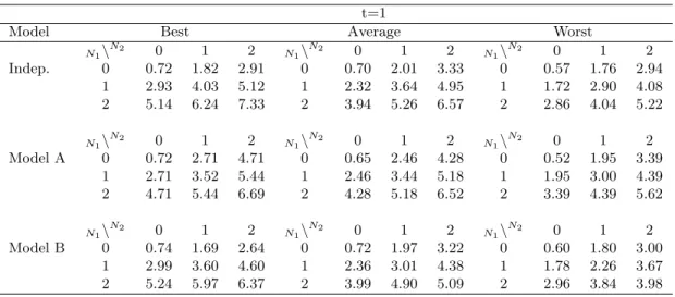
The a posteriori risk factors, calculated as mentioned, for three different profiles (Best, Average and Worst) and t = 1 are compared in Table 4 for Independent model, model A and model B. Putting aside model A, and focusing on model B as opposed to the independence
case, the a posteriori risk factors located at the first row (N1 = 0) or at the first column
(N2 = 0) do not diverge significantly between model B and the independence case. However,
thea posteriori risk factors corresponding to policyholders that report at least one claim of each type are significantly different. In particular, relaxing the independence assumption leads to a lower a posteriori risk factors. For model A, we can observe the same behaviour even though its specific symmetrical nature. Concentrating on the differences between the three profiles, the bivariate experience rating models behave in the same manner as univariate models, that is, producing largera posteriori risk factors for those policyholders with a lower prior premium.
To show the behaviour of thea posteriori risk factors over time, Table 5 displays the results for twelve years in the case where a policyholder has reported one claim of each type during the first year and no more claims are ever reported by him. For model B, we have found that the difference mentioned above for t = 1 between the a posteriori risk factors of model B and the corresponding factors of the independence case is attenuated over time in all cases. For model A, this conduct is not equal for the three profiles.
5
Conclusions
We introduce here two different bivariate experience rating models that integrate the a priori
ratemaking based on the bivariate Poisson regression model presented in Berm´udez (2009) to account for the dependence between two type of claims. Using the standard Bayesian procedure, we extend the existing literature for the univariate case to the bivariate case obtaining posterior premiums anda posteriori risk factors for the bivariate experience rating models proposed here. The two bivariate models proposed here may respond to different market needs. As model A uses a common random effect, this model can be used when the insurer is not interested in differentiating the posterior ratemaking for the two type of claims, but taking into account the dependence between them. If, on the other hand, the insurer prefers different posterior ratemaking for each type of claim, model B will be the best option.
When the independence assumption is relaxed, the main consequence for posterior ratemak-ing is that the a posteriori risk factors corresponding to policyholders that report at least one claim of each type are significantly reduced compared with those factors derived from the inde-pendence case. This is particularly true with regard to those policyholders with lower a priori
premiums (good drivers) since they will present largera posteriori risk factors than policyhold-ers classified as bad drivpolicyhold-ers. From the numerical application is also derived that this reduction ina posteriori risk factors is attenuated over time.
It is therefore worth giving careful consideration to this issue. The idea behind a posteriori
ratemaking is fitting an individual premium based on the claim experience for each insured party on the assumption that the unknown risk characteristics (i.e. driving ability, obedience of traffic regulations) are revealed by the number of claims reported by the policyholders. It is reasonable to believe that some of these characteristics simultaneously affect the two type of claims. We interpret the reduction ina posteriori risk factors when the independence assumption is relaxed as the effect of taking into account this latter fact. That is, the bivariate experience rating models do not recharge twice for the same unknown risk characteristic.
Finally, we would like to mention various ways in which this paper might be extended. First, zero-inflated bivariate Poisson models presented in Berm´udez (2009) can be also used and derived. Second, finite mixtures models presented in Berm´udez and Karlis (2012) can be also used and derived but they will be much more complicated, but still tractable. Third, although in the present paper we limit our analysis to the bivariate case, it could be extended to include larger dimensions, following the general model presented by Berm´udez and Karlis (2011). Fourth, in model B, instead of independent random effects, we can also assume some dependence and proceed. Finally, we could replace the Gamma assumption with an inverse Gaussian one (or any other mixing distribution) easily.
References
Berm´udez, L. (2009). A priori ratemaking using bivariate Poisson regression models. Insurance: Mathematics and Economics, 44(1), 135-141.
Berm´udez L., & Karlis, D. (2011). Bayesian multivariate Poisson models for insurance ratemak-ing. Insurance: Mathematics and Economics, 48(2), 226-236.
Berm´udez L., & Karlis, D. (2012). Finite mixture of bivariate Poisson regression models with an application to insurance ratemaking. Computational Statistics and Data Analysis, 56, 3988-3999.
B¨uhlmann, H., & Gisler, A. (2005). A Course in Credibility Theory and its Applications. Berlin: Springer.
Denuit, M., Marechal, X., Pitrebois, S., & Walhin, J.-F. (2007). Actuarial Modelling of Claim Counts: Risk Classification, Credibility and Bonus-Malus Systems. New York: Wiley. G. Dionne, G., & Vanasse, C. (1989). A generalization of actuarial automobile insurance rating
models: the negative binomial distribution with a regression component. ASTIN Bulletin, 19(2), 199-212.
Englund, M., Guill´en, M., Gustafsson, J., Nielsen, L.H., & Nielsen, J.P. (2008). Multivariate latent risk: A credibility approach. ASTIN Bulletin, 38(1), 137-146.
Frees, E.W. (2003). Multivariate credibility for aggregate loss models. North American Actu-arial Journal, 7(1), 13-27.
Johnson, N., Kotz, S., & Balakrishnan, N. (1997). Multivariate Discrete Distributions. New York: Wiley.
Karlis, D., & Tsiamyrtzis, P. (2008). Exact bayesian modeling for bivariate poisson data and extensions. Statistics and Computing, 18(1), 27-40.
Kocherlakota, S., & Kocherlakota, K. (1992). Bivariate Discrete Distributions, Statistics: text-books and monographs, volume 132. New York: Markel Dekker.
Pinquet, J. (1998). Designing optimal bonus-malus systems from different types of claims.
ASTIN Bulletin, 28(2), 205-220.
Subrahmaniam, K. (1966). A test for ”intrinsic correlation” in the theory of accident proneness.
Table 1: Cross-tabulation of data N1 N2 0 1 2 3 4 5 6 0 24408 1916 296 69 12 6 0 1 1068 317 61 21 6 2 2 2 203 71 18 6 2 1 1 3 49 14 8 3 3 1 0 4 11 6 2 0 1 0 0 5 2 0 0 0 0 0 1 6 1 0 0 1 0 0 0 8 0 0 1 0 0 0 0
N1: number of claims for third-party liability. N2: number of claims for the rest of guarantees.
Table 2: Comparison of a priori ratemaking
Best Average Worst
Model Mean Variance Mean Variance Mean Variance
DP 0.1624 0.1624 0.2106 0.2106 0.3634 0.3634
BP 0.1570 0.1883 0.2078 0.2391 0.3525 0.3838
DP: Independence Poisson; BP: Bivariate Poisson.
Table 3: Prior parameter estimation
Model Prior distribution Parameter estimation
Indep. Θ1∼Gamma(a, a) ˆa= 0.1629 Θ2∼Gamma(b, b) ˆb= 0.3288 A Θ∼Gamma(α, α) αˆ= 0.3598 B Θ1∼Gamma(α1, α1) αˆ1= 0.1309 Θ2∼Gamma(α2, α2) αˆ2= 0.3101 Θ3∼Gamma(α3, α3) αˆ3= 0.0555
Table 4: Comparison ofa posteriori ratemaking
t=1
Model Best Average Worst
N1\ N2 0 1 2 N1\ N2 0 1 2 N1\ N2 0 1 2 Indep. 0 0.72 1.82 2.91 0 0.70 2.01 3.33 0 0.57 1.76 2.94 1 2.93 4.03 5.12 1 2.32 3.64 4.95 1 1.72 2.90 4.08 2 5.14 6.24 7.33 2 3.94 5.26 6.57 2 2.86 4.04 5.22 N1\ N2 0 1 2 N1\ N2 0 1 2 N1\ N2 0 1 2 Model A 0 0.72 2.71 4.71 0 0.65 2.46 4.28 0 0.52 1.95 3.39 1 2.71 3.52 5.44 1 2.46 3.44 5.18 1 1.95 3.00 4.39 2 4.71 5.44 6.69 2 4.28 5.18 6.52 2 3.39 4.39 5.62 N1\ N2 0 1 2 N1\ N2 0 1 2 N1\ N2 0 1 2 Model B 0 0.74 1.69 2.64 0 0.72 1.97 3.22 0 0.60 1.80 3.00 1 2.99 3.60 4.60 1 2.36 3.01 4.38 1 1.78 2.26 3.67 2 5.24 5.97 6.37 2 3.99 4.90 5.09 2 2.96 3.84 3.98
Table 5: A posteriori risk factors for policyholders reporting one claim of each type
Best Average Worst
Ind. A B Ind. A B Ind. A B
t= 1 4.03 3.52 3.60 3.64 3.44 3.01 2.90 3.00 2.26 t= 2 3.13 2.91 2.94 2.78 2.68 2.44 2.04 2.07 1.72 t= 3 2.57 2.45 2.48 2.25 2.17 2.04 1.57 1.58 1.38 t= 4 2.19 2.11 2.14 1.89 1.82 1.75 1.28 1.27 1.15 t= 5 1.91 1.85 1.89 1.63 1.57 1.53 1.07 1.07 0.99 t= 6 1.69 1.64 1.69 1.43 1.37 1.36 0.93 0.92 0.87 t= 7 1.52 1.48 1.53 1.28 1.22 1.23 0.82 0.80 0.78 t= 8 1.38 1.34 1.40 1.15 1.10 1.12 0.73 0.72 0.70 t= 9 1.26 1.23 1.28 1.05 1.00 1.02 0.66 0.65 0.64 t= 10 1.17 1.14 1.19 0.96 0.92 0.95 0.60 0.59 0.59 t= 11 1.08 1.05 1.11 0.89 0.85 0.88 0.55 0.54 0.54 t= 12 1.01 0.98 1.04 0.83 0.79 0.82 0.51 0.50 0.50