Guay: Département de sciences économiques, Université du Québec à Montréal, Québec, Canada, CIRPÉE and CIREQ
Lamarche: Department of Economics, Brock University, St. Catharines, Ontario, Canada [email protected]
The first author gratefully acknowledges financial support of le Fonds québécois de la recherche sur la société et la culture (FQRSC). The first and second authors are thankful for the financial support of the Social Sciences and Humanities Research Council of Canada (SSHRC). We are grateful to Chuan Goh for his comments and also for the comments of participants at the CIREQ Conference on Generalized Method of Moments, Montréal, 2007, ESEM Budapest 2007 and CEA meeting 2007.
Cahier de recherche/Working Paper
08-33
The Information Content of Implied Probabilities to Detect Structural
Change
Alain Guay
Jean-François Lamarche
Octobre/October 2008
Abstract:
This paper proposes Pearson-type statistics based on implied probabilities to detect
structural change. The class of generalized empirical likelihood estimators (see Smith
(1997)) assigns a set of probabilities to each observation such that moment conditions
are satisfied. These restricted probabilities are called implied probabilities. Implied
probabilities may also be constructed for the standard GMM (see Back and Brown
(1993). The proposed test statistics for structural change are based on the information
content in these implied probabilities. We consider cases of structural change with
unknown breakpoint which can occur in the parameters of interest or in the
overidentifying restrictions used to estimate these parameters. The test statistics
considered here have good size and power properties.
Keywords:
Generalized empirical likelihood, generalized method of moments,
parameter instability, structural change
1 Introduction
This paper proposes structural change tests based on implied probabilities resulting from estimation methods based on unconditional moment restrictions. The Generalized Method of Moments (GMM) is the standard method to estimate parameters of interest through moment restrictions. However, Monte Carlo results reveal that the GMM estimators may be seriously biased in small sample.1 Recently, a number of alternative estimators to GMM have been proposed. Hansen, Heaton and Yaron (1996) suggested the continuous updated estimator (CUE) which shares same objective function that the GMM but with a weighting matrix depending on the parameters of interest. The empirical likelihood (EL) (see Qin and Lawless (1994)) and the exponential tilting (ET) estimators (see Kitamura and Stutzer (1997)) have also been proposed. Kitamura (2001) showed that tests for the validity of moment restrictions based on EL have optimal properties in terms of large deviations. In particular EL tests are shown to be more powerful than other standard tests. These alternative estimators are special cases of the generalized empirical likelihood (GEL) class considered by Smith (1997) and may be shown to be based on the Cressie and Read (1984) family of power divergence criteria. Newey and Smith (2004) showed (in an i.i.d. setting) that, although estimators based on the GMM, EL, ET or that are CUE have the same first order asymptotic distribution, they have different higher order asymptotic properties. Amongst their findings it is shown that the expression for the second order asymptotic bias of GEL has fewer components than the one of GMM (with EL having the fewest). Anatolyev (2005) extended the Newey and Smith setting to allow for weakly dependent data correlation and show that the asymptotic bias of smoothed GEL estimators is less than the GMM estimators especially with many moment conditions.
GEL estimators assign a probability to each observation such that the moment conditions are satisfied (see Smith (2004)). This resulting empirical measure is called implied probabilities. Implied probabilities may also be constructed for the standard GMM as shown by Back and Brown (1993). The interpretation of the implied probabilities is the following: less weight is assigned to an observation for which the moment restrictions are not satisfied at the estimated values of the parameters and more weight to an observation for which the moment restrictions are satisfied. As suggested by Back and Brown (1993), implied prob-abilities may then provide a useful diagnostic device for the model specification. In particular, implied probabilities may contain interesting information to detect instability in the sample. Consequently, we propose the use of these weights in detecting an unknown structural change in the model. Antoine, Bon-nal and Renault (2007) use the weights given by implied probabilities to propose a three-step estimation procedure asymptotically higher equivalent to empirical likelihood. Schennach (2004) also discusses the use of these weights in the context of model misspecification. Ramalho and Smith (2005) considered Pearson-type test statistics (statistics based on the difference between restricted and unrestricted
mators of the weights) for the validity of moment restrictions and parametric restrictions using implied probabilities.
The proposed test statistics to detect structural change are based on different measures of the dis-crepancy between these implied probabilities and the unconstrained empirical probabilities T1. These test statistics fall in three categories: 1) general structural change tests to detect instability in the identifying restrictions and in the overidentifying restrictions; 2) structural change tests specially designed to de-tect instability in the identifying restrictions (see for example Andrews (1993)) and 3) structural change tests to detect instability in the overidentifying restrictions (see for example Hall and Sen (1999)). The asymptotic distribution of the statistic tests is derived for the case of unknown breakpoint under the null and under the alternative hypotheses. In a simulation study, we find that targeted tests based on implied probabilities performed quite well if the structural change corresponds to the target. That is, if instability is present in the identifying restrictions or in the overidentifying restrictions, then the targeted tests have size and power that are at least as good as those of the more standard tests. General tests for structural change have size and power properties that are between those of the targeted tests. Overall the test statistics based on implied probabilities considered in this paper have a nice intuitive appeal, are based on an estimation method that has been shown to have nice higher order asymptotic properties and are relatively easy to compute.
The paper is organized as follows. A discussion on the GMM and GEL estimators are presented in section 2. Section 3 presents formally the full-sample and partial-sample GMM and GEL estimators. Section 4 presents the test statistics proposed based on the implied probabilities. The simulation results are in Section 5 while the proofs are in the Appendix.
2 Discussion of GMM and GEL Estimators
In this section we present the estimators used in this paper. We start with an entropy-based formula-tion of the problem which puts emphasis on the informaformula-tional content of the estimated weights. We then move to the more recent GEL formulation (see Newey and Smith (2004) and Smith (2004)).
We consider a random variable{xt: 1≤t≤T, T ≥1}. Suppose we haveq×1 vector function of the data g(xt, θ) which depends on some unknown p-vector of parametersθ ∈Θ with Θ⊂Rp and that in the population their expected value is 0, namely
E[g(xt, θ0)] = 0
Along this paper we consider the overidentifying case withq > p.
The standard GMM estimators (Hansen (1982)) are obtained as the solution of ˜
θT =argmin θ∈ΘgT(θ)
0W TgT(θ)
where WT is a random positive definite symmetric q×q matrix and gT(θ) = T1P T
t=1g(xt, θ). The optimal weighting matrix is defined to be the inverse of the covariance matrix of the moment conditions,
WT = Ω−T1where ΩT is a consistent estimator of Ω = lim T→∞V ar 1 √ T T X t=1 g(xt, θ) ! .
The optimal weighting matrix can be estimated consistently using methods developed by Gallant (1987), Andrews and Monahan (1992) and Newey and West (1994), among several others.
We note that, in the GMM criterion function, the moment conditions receive equal weight (1/T) for each observations. Back and Brown (1993) derive a set of implicit weights using the GMM estimators given by πt(θ) = 1 T − 1 T−p[JtT(θ)−JT(θ)] 0ˆ ΩT(θ)−1gT(θ) (1) withJT(θ) = T1P T t=1JtT(θ) and JtT(θ) = T X j=1 κ(|t−j|)g(xt−j, θ)
whereκ(|t−j|) is a real valued weighting function. The following estimator ˆ ΩT(θ) = 1 T−p T X t=1 JtT(θ)g(xt, θ)0
is a consistent and positive definite estimator of the variance-covariance matrix and it has the usual form of a heteroskedasticity and autocorrelation consistent (HAC) weight matrix for standard kernelsκ(|t−s|) considered in the vast literature on consistent estimation of variance-covariance matrix (see e.g. Andrews (1991), Newey and West (1987) and Newey and West (1994)). The implied probabilities defined above are the empirical measure that ensures that moment conditions are satisfied in the sample.
Now letting theT-vector ofexplicit weights (explicit because the weights are used directly in estima-tion) be{πt: 1≤t≤T, T ≥1} we can recast the population moment conditions as
Eπ[g(xt, θ0)] = 0.
The vector πis determined by finding the most probable data distribution of the outcomes given the data. We can think ofπas containing information on the content of the moment conditions. Therefore,
g(x, θ) is viewed as a message. That is, whenπis small, the message is informative and vice-versa. This relation is summarized by the functionf(π) =−lnπ. The average information is then
S(π)≡Eπf(π) =− T
X
t=1
In this case,S(π) can be interpreted as the entropy measure of Shannon (1948) and it captures the degree of uncertainty in the distributionπwith respect to whether or not the distribution is concentrated or dispersed. The vectorπis obtained by maximizing entropy
maxS(π) =− T X t=1 πtlnπt, subject toPT t=1πt= 1 andP T t=1πtg(xt, θ) = 0.
With no constraint, we get πt= 1/T ∀t, the maximally uninformative uniform distribution, while with constraints, we want to chooseπt to be as maximally uninformative as the moment conditions will allow. We do not want to assert more about the distribution than is known via the moment conditions. In this sense, the probabilities make use of all the information that is available, and nothing more. In particular, we focus on detecting a structural change in the moment conditions. With no structural change, the weights will fluctuate around 1/T, otherwise the entropy formulation will attempt to reduce the weight on the observation characterized by the change, and at the same time put more weights on the remaining observations so as to makeS(π) as large as possible.
We can transpose this formulation using the Kullback and Leibler (1951) information criterion which measures the discrepancy between two distributions p and π. If the subject distribution is π and the reference distribution ispt= 1/T,∀twe have
KLIC(π, p= 1/T) = T X t=1 πt[ln(πt)−ln(1/T)] = T X t=1 πtln(πt) + ln(T).
So that maximizing entropy is equivalent to minimizing theKLIC(π, p= 1/T). Estimates ofπ, given
θ, are obtained by maximizing S(π) (or by minimizingKLIC(π, p= 1/T)) subject to the weighted zero functions and the probability constraint. The solution to the Lagrangian yields
πtET(θ) = exp(γ 0g(x
t, θ))
PT
t=1exp(γ0g(xt, θ))
where theq-vectorγcontains the Lagrange multipliers and as such measure the degree of departure from zero of the moment conditions andET stands for exponential tilting (see Kitamura and Stutzer (1997)). Estimates of θ are obtained by substituting π in S(π), maximizing it with respect to γ and then with respect toθ (see for example Kitamura and Stutzer (1997)).
If we interchange the subject/reference distributions we get
KLIC(p= 1/T, π) = T
X
t=1
(1/T)[ln(1/T)−ln(πt)]
and the solution to the optimization problem yields a different set of weights given by
πtEL(θ) = 1
T[1 +γ0g(x t, θ)]
where ELstands for empirical likelihood (see Qin and Lawless (1994) for example). When we evaluate the weights at some estimators we obtainπtET(˜θT) andπtEL(˜θT). Recently, Schennach (2004) combined ET and EL into the ETEL estimator that combines the advantages of each approach.
We mentioned in the introduction that less weight is assigned to an observation for which the moment conditions are not satisfied. In this section we have seen that the vector π contains all the relevant information with respect to the moment conditions. We now provide a graphical intuition on the use of the weights in the detection of a structural change. We consider a small simulation study that contains three examples that have been studied in the structural change and entropy literature. The first example, which encompasses three cases, is similar to the one used by Imbens, Spady and Johnson (1998) and consists of estimating a single parameter,θ, with 2 moment conditions:
E[xt−θ] = 0 and E
(xt−θ)2−4
= 0
with a sample of 100 observations andxt=θt+twheret∼N(0,4). We consider a pulse, a break and a regime shift cases. In the pulse case we haveθt= 5 fort= 50 andθ= 10 otherwise. For the break case we haveθt = 10 fort≤20 and t >80 while θt= 15 for 21≤t≤80. Finally, the regime shift case has
θt= 10 fort≤20 andθt= 15 otherwise. In these cases, structural change occurs via the parameters and can be tested using procedures proposed by Andrews (1993) and by Andrews and Ploberger (1994).
In contrast, the next two examples consist of structural change through the moment conditions. Following Hall and Horowitz (1996) and Gregory, Lamarche and Smith (2002) we study a simulated environment with CRRA preferences and making a distributional assumption on consumption growth,xt, with i.i.d data andT = 100. In particular, we assume that consumption growth follows aN(0, σ2= 0.16). There is a single parameter to be estimated,γ, the coefficient of CRRA and two moment conditions are used:
Etexp[−γlnxt+1−9σ2/2 + (3−γ)zt] = 1
Etztexp[−γlnxt+1−9σ2/2 + (3−γ)zt−1] = 0
with zt ∼N(0, σ2). The moment conditions are satisfied when γ = 3. The structural break occurs in period 51 and is summarized by a shift inγ from 3 to 4.
Lastly, as in Ghysels, Guay and Hall (1997), we have the estimation of an autoregressive parameter using two moment conditions when the data generating process is anAR(1) (xt=ρxt−1+t), fort≤50, and anARM A(1,2) otherwise (xt=ρxt−1+t+ 0.5t−2). There are 100 observations andt∼N(0,1). The two instruments used are the first and second lags ofxt. The two moment conditions are then:
E[xt−1(xt−ρxt−1)] = 0
The instability occurs because the second moment condition is violated aftert >50.
Figure 1 shows the average of the vector of implied probabilities πover 10,000 replications. The key feature of these panels is that when there is no break, the weights fluctuate around 1/T = 1/100 (upper right panel). With a structural break in the parameter or in the moment conditions, however, more weight is given to observations (and moment conditions) for which there is no break while less weight is assigned to an observation which violates the moment conditions. This simple simulation study clearly show that implied probabilities contain interesting information to detect structural change. In this paper, we examine the information contained in the estimated implied probabilities to detect structural change and propose test statistics based on some function of implied probabilities.
Now following the recent econometric literature (see Caner (2004), Newey and Smith (2004), Smith (2004), Caner (2005), Guggenberger and Smith (2007) and Ramalho and Smith (2005)) on GEL we let
ρ(φ) be a function of a scalar φthat is concave on its domain, an open interval Φ that contains 0. Also, let ˜ΓT(θ) ={γ:γ0g(xt, θ)∈Φ, t= 1, . . . , T}. Then, the GEL estimator is a solution to the problem
˜ θT = arg min θ∈Θ sup γ∈˜ΓT(θ) T X t=1 [ρ(γ0g(xt, θ))−ρ0] T
whereρj() =∂jρ()/∂φjandρj =ρj(0) forj= 0,1,2, . . .. Under this formulation a number of estimators can be obtained. First, the ET estimator of θ is found by setting ρ(φ) = −exp(φ). Second, the EL estimator of θ by setting ρ(φ) = ln(1−φ). Third, the continuously updated estimator, as opposed to the two-step estimator presented above, of Hansen et al. (1996) can also be obtained from the GEL formulation by using a quadratic function forρ(φ) =−(1 +φ)2/2.
As in the GMM context an adjustment for the dynamic structure of g(xt, θ) can also be made in the GEL context ( see Kitamura and Stutzer (1997), Smith (2000), Smith (2004) and Guggenberger and Smith (2007)). The adjustment consists of smoothing the original moment conditions g(xt, θ). Defining the smoothed moment conditions as
gtT(θ) = 1 ST t−1 X s=t−T k s ST g(xt−s, θ)
for t = 1, . . . , T and ST is a bandwidth parameter, k(·) a kernel function and we define where kj =
R∞
−∞k(a)
jda. In the time series context, the criteria is then given by: T X t=1 [ρ(kγ0g tT(θ))−ρ0] T wherek=k1 k2 (see Smith (2004)).
3 Full and Partial-Samples GMM and GEL Estimators
To establish the asymptotic distribution theory of tests for structural change in the parameters based on implied probabilities we need to elaborate on the specification of the parameter vector in our generic setup. We will consider parametric models indexed by parameters (β, δ). With no structural change we define a vector of parameters (β, δ)⊂B×∆∈Rp withp=r+ν. Following Andrews (1993) we make a distinction between pure structural change when no subvectorδappears and the entire parameter vector is subject to structural change under the alternative and partial structural change which corresponds to cases where only a subvectorβis subject to structural change under the alternative. The generic null can be written as follows:
H0:βt=β0 ∀t= 1, . . . , T. (2)
The tests that we will consider assume as alternative that at some point in the sample there is a single structural break, like for instance:
βtT =
β1(s) t= 1, ...,[T s]
β2(s) t= [T s] + 1, ..., T
wheresdetermines the fraction of the sample before and after the assumed breakpoint and [.] denotes the greatest integer function. The separation [T s] represents a possible breakpoint which is governed by an unknown parameters. Hence, we will consider a setup with a parameter vector which encompasses any kind of partial or pure structural change involving a single breakpoint. In particular, we consider a 2r+ν
dimensional parameter vectorθ= (β01, β20, δ0)0whereβ1andβ2∈B⊂Rrandθ∈Θ =B×B×∆⊂R2r+ν. The parameters β1 and β2 apply to the samples before and after the presumed breakpoint and the null implies that:
H0:β1=β2=β0. (3)
We will formulate all our models in terms ofθ. Special cases could be considered whenever restrictions are imposed in the general parametric formulation. One such restriction would be that θ0 = (β00, β00)0, which would correspond to the null of a pure structural change hypothesis. Once we have defined the moment conditions we will also translate this into overidentifying restrictions and relate it to structural change tests, following the analysis of Sowell (1996a) and Hall and Sen (1999).
3.1
Definitions
We need to impose restrictions on the admissible class of functions and processes involved in estimation to guarantee well-behaved asymptotic properties of GMM and GEL estimators using the entire data sample or subsamples of observations. A set of regularity conditions is required to obtain weak convergence of partial-sample GMM and GEL estimators to a function of Brownian motions. To streamline the
presentation we provide a detailed description of them in Appendix 7.1. We now formally define the standard GMM estimator using the full sample.
Definition 3.1. The full-sample General Method of Moments estimator {( ˜βT,δ˜T)} is a sequence of
random vectors such that:
˜ βT0,δ˜0T 0 =arg min (β,δ)∈B×∆gT(β, δ) 0Wˆ TgT(β, δ)
whereWˆT is a random positive definite symmetricq×qmatrix.
The optimal weighting matrix W is defined to be the inverse of Ω which is defined as: Ω = lim T→∞V ar 1 √ T T X t=1 g(xt, β0, δ0) ! .
The optimal weighting matrix can be estimated consistently using methods developed by Gallant (1987), Andrews and Monahan (1992) and Newey and West (1994), among several others.
To characterize the asymptotic distribution we define the following matrices:
Gβ= lim T→∞ 1 T T X t=1 E∂g(xt, β0, δ0)/∂β0∈Rq×r, Gδ = lim T→∞ 1 T T X t=1 E∂g(xt, β0, δ0)/∂δ0 ∈Rq×ν, G= [ Gβ Gδ ]∈Rq×p.
wherep=r+ν. Finally, let ˜θT =
˜
βT0,β˜T0 ,δ˜T0
0
be a 2r+ν-vector. Hereafter, the vector ˜θT is called the full-sample estimator ofθ. This restricted estimator is consistent only under the null thatβ1=β2.
Several tests for structural change involve partial-sample GMM estimators defined by Andrews (1993). We consider again the two subsamples, the first based on observations t = 1, . . . ,[T s] and the second coveringt= [T s] + 1, . . . , T where s∈S⊂(0,1). The partial-sample GMM estimators fors∈S based on the first and the second subsamples are formally defined as:
Definition 3.2. A partial-sample General Method of Moments estimator{θˆT(s)}is a sequence of random
vectors such that:
ˆ
θT(s) =argmin
θ∈ΘgT(θ, s) 0Wˆ
T(s)gT(θ, s)
for alls∈S. Definegt(θ, s) = (g(xt, β1, δ)0,00) 0
∈R2q×1fort= 1, . . . ,[T s]andg
t(θ, s) = (00, g(xt, β2, δ)0) 0
∈
R2q×1 fort= [T s] + 1, . . . , T such that
gT(θ, s) = 1 T T X t=1 gt(θ, s) = 1 T [T s] X t=1 h g(x t, β1, δ) 0 i + 1 T T X t=[T s]+1 h 0 g(xt, β2, δ) i
andWˆT(s) is a random positive definite symmetric2q×2q matrix. According to the definition above ˆθT(s) =
ˆ
β1T(s)0,βˆ2T(s)0,δˆT(s)0
0
is a 2r+ν-vector with an es-timator ˆβ1T(s) that uses the first subsamplet = 1, . . . ,[T s], an estimator ˆβ2T(s) that uses the second subsamplet= [T s] + 1, . . . , T and an estimator ˆδT(s) that uses all the sample.
The partial-sample optimal weighting matrix is defined as the inverse of Ω(s) where
Ω(s) = lim T→∞V ar 1 √ T " P[T s] t=1g(xt, β0, δ0) PT t=[T s]+1g(xt, β0, δ0) #!
which under the null (3) is asymptotically equal to
Ω(s) =h s0Ω (1−0s)Ω i. We also define G(s) = sGβ 0 sGδ 0 (1−s)Gβ (1−s)Gδ ∈R2q×(2r+ν).
In the GEL setting, the parameter vector is augmented by a vector of auxiliary parametersγ where each element of this vector is associated to an element of the smoothed moment conditionsgtT(θ). Under the null of no structural change relative to the specification of the model, the generic null hypothesis for this vector of auxiliary parameters can be written as follows:
H0:γt=γ0= 0 ∀t= 1, . . . , T. (4)
As for the parameter vectorβ, the tests that we will consider assume as alternative that at some point in the sample there is a single structural break, namely:
γt=
γ1 t= 1, ...,[T s]
γ2 t= [T s] + 1, ..., T.
Thus under the null of no structural change H0 : γ1 =γ2 =γ0 = 0. Guay and Lamarche (2007) show that a structural change inγis associated with instability in the overidentifying restrictions.
We now formally define the GEL estimator using the full sample.
Definition 3.3. Let ρ(φ) be a function of a scalar φ that is concave on its domain, an open interval
Φ that contains 0. Also, let Γ˜T(β, δ) = {γ : kγ0gtT(β, δ) ∈ Φ, t = 1, . . . , T} with k = kk12. Then, the
full-sample GEL estimator{θ˜T} is a sequence of random vectors such that:
˜ βT0 ,˜δT0 0 = arg min (β,δ)∈B×∆ sup γ∈ΓeT(β,δ) T X t=1 [ρ(kγ0gtT(β, δ))−ρ0] T
The criteria is normalized so thatρ1 =ρ2=−1 (see Smith (2004)). As mentioned earlier, the GEL estimator admits a number of special cases recently proposed in the econometrics literature. The CUE of Hansen, Heaton and Yaron (1996) corresponds to the following quadratic function ρ(φ) =−(1 +φ)2/2. The EL estimator (Qin and Lawless, 1994) is a GEL estimator withρ(φ) = ln(1−φ). The ET estimator (Kitamura and Stutzer, 1997) is obtained withρ(φ) =−exp(φ).
More precisely, the GEL estimator is obtained as the solution to a saddle point problem. Firstly, the criterion is maximized for given vector (β, δ). Thus,
˜ γT(β, δ) = arg sup γ∈˜Γ(β,δ) T X t=1 [ρ(kγ0gtT(β, δ))−ρ0] T .
Secondly, the GEL estimatorβ˜T0 ,˜δT0
0
is given by the following minimization problem:
˜ βT0,˜δT0 0= arg min (β,δ)∈B×∆ T X t=1 ρ kγ˜T(β, δ) 0 gtT(β, δ) −ρ0 T .
From now on, following Kitamura and Stutzer (1997) and Guggenberger and Smith (2007) we focus on the truncated kernel defined by
k(x) = 1 if|x| ≤1 andk(x) = 0 otherwise to obtain the following smoothed moment conditions
gtT(β, δ) = 1 2KT + 1 KT X j=−KT g(xt−j, β, δ).
To handle the endpoints in the smoothing we use the approach of Smith (2004) and Guggenberger and Smith (2007) which sets
gtT(β, δ) = 1 2KT + 1 min{t−1,KT} X j=max{t−T ,−KT} g(xt−j, β, δ).
We can easily show for this kernel thatk= k1
k2 = 1. A consistent estimator of the long run covariance matrix is then given by:
˜ ΩT(β, δ) = 2KT + 1 T T X t=1 gtT(β, δ)gtT(β, δ)0.
The weighting matrix thus obtained using this type of kernel is similar to the one obtained with the Bartlett kernel estimator of the long run covariance matrix of the moment conditions (see Smith (2004)). Define also the derivatives of the smoothed moment conditions as:
GtT(β, δ) = 1 2KT + 1 KT X j=−KT ∂g(xt−j, β, δ) ∂(β0, δ0) .
Now consider a possible breakpoint [T s]. Define the vector of auxiliary parametersγ(s) = (γ1(s)0, γ2(s)0)0 whereγ1is the vector of the auxiliary parameters for the first part of the sample e.g.t= 1, . . . ,[T s] and
γ2 for the second part of the sample;t= [T s] + 1, . . . , T. The partial-sample GEL estimators fors∈S based on the first and the second subsamples are formally defined as:
Definition 3.4. Let ρ(φ) be a function of a scalar φthat is concave on its domain, an open interval Φ
that contains 0. Also, letΓˆT(θ, s) ={γ(s) = (γ1(s)0, γ2(s)0)0:kγ(s)0gtT(θ, s)}. A partial-sample General
Empirical Likelihood (PS-GEL) estimator{θˆT(s)}is a sequence of random vectors such that: ˆ θT(s) = arg min θ∈Θ sup γ(s)∈ˆΓ T(θ,s) T X t=1 [ρ(kγ(s)0g tT(θ, s))−ρ0] T = arg min θ∈Θ sup γ(s)∈ˆΓ T(θ,s) [T s] X t=1 [ρ(kγ10gtT(β1, δ))−ρ0] T + T X t=[T s]+1 [ρ(kγ20gtT(β2, δ))−ρ0] T
for alls∈S, wheregtT(θ, s) = (gtT(β1, δ)0,00)0∈R2q×1fort= 1, . . . ,[T s]andgtT(θ, s) = (00, gtT(β2, δ)0)0∈
R2q×1 fort= [T s] + 1, . . . , T with γ(s) = (γ1(s)0, γ2(s)0)0 ∈R2q×1.
To be more precise, the first order conditions corresponding to the Lagrange multiplierγare obtained from the maximization of the partial-sample GEL criterion for a givenβ1, β2, δ. Thus,
ˆ γ1T(β1, δ) = arg sup γ1∈ˆΓ1T(β1,δ) [T s] X t=1 [ρ(kγ1(β1, δ)0gtT(β1, δ))−ρ0] T , ˆ γ2T(β2, δ) = arg sup γ2∈ˆΓ2T(β2,δ) T X t=[T s]+1 [ρ(kγ2(β2, δ)0gtT(β2, δ))−ρ0] T . with ˆΓ1T(β1, δ) ={γ1:kγ10gtT(β1, δ)∈Φ, t= 1, . . . ,[T s]}and ˆΓ2T(β2, δ) ={γ2:kγ20gtT(β2, δ)∈Φ, t= [T s] + 1, . . . , T}.
We now present the corresponding implied probabilities defined by Back and Brown (1993) and Smith (2004) for the most commonly used full and partial-sample estimators. Following Back and Brown (1993), the full-sample GMM implied probabilities are defined as:
πt(˜θT) = 1 T − 1 T h JtT(˜θT)−JT(˜θT) i0 ˆ ΩT(˜θT)−1gT(˜θT) withJT(˜θT) = T1P T t=1JtT(˜θT) and JtT(˜θT) = T X j=1 κ(|t−j|)g(xt−j,θ˜T)
whereκ(|t−j|) is a real valued weighting function. In practice, however, some of the estimated probabil-ities may be negative in finite sample although these probabilprobabil-ities are asymptotically positive. Antoine,
Bonnal, and Renault (2007) proposed a shrinkage procedure defined as a weighted average of the stan-dard 2S-GMM’s implied probabilities (1/T) and the computed implied probabilities to guarantee the non-negativity of these implied probabilities in finite sample.
The general formula of the implied probabilities for the full-sample GEL estimator is defined by the following ratio (see Smith, 2004):
πGELt (˜θT) = ρ1 ˜ γ0TgtT(˜θT) PT t=1ρ1 ˜ γT0gtT(˜θT) .
Implied probabilities for the full-sample ET, EL and CUE estimators with the smoothed moment conditions are respectively given by:
πETt (˜θT) = exp[ ˜γT0gtT(˜θT)] PT t=1exp[˜γ 0 TgtT(˜θT)] , πELt (˜θT) = 1 T[1 + ˜γ0TgtT(˜θT)] , and πCU Et (˜θT) = 1 T − 1 TgtT(˜θT) " 1 T T X t−1 gtT(˜θT)gtT(˜θT)0 #−1 1 T T X t=1 gtT(˜θT). Note that 2K+1 T PT t−1gtT(˜θT)gtT(˜θT)0 is a consistent estimator of Ω.
The corresponding unrestricted partial-sample GMM implied probabilities are defined for s∈S as:
πt(ˆθT(s), s) = 1 T − 1 T h JtT(ˆθT(s), s)−JT(ˆθT(s), s) i0 ˆ ΩT(s)−1gT(ˆθT(s), s) withJT(ˆθT(s), s) = T1 P T t=1JtT(ˆθT(s), s) and JtT(ˆθT(s), s) = T X j=1 κ(|t−j|)gt−j(ˆθT(s), s)
where κ(|t−j|) is a real valued weighting function and gT(ˆθT(s), s) = T1 P T
t=1gt(ˆθT(s), s). The general formula for the unrestricted partial-sample implied probabilities for the GEL are defined fors∈S as:
πtGEL(ˆθT(s), s) = ρ1 ˆ γT(s)0gtT(ˆθT(s), s) PT t=1ρ1 ˆ γT(s)0gtT(ˆθT(s), s) . (5)
For example, in the case of t between observations 1 and [T s], we get for the unrestricted implied probabilities att: πGELt ( ˆβ1T(s),δˆT(s), s) = ρ1 ˆ γ1T(s)0gtT( ˆβ1T(s),δˆT(s)) PT t=1ρ1 ˆ γ1T(s)0gtT( ˆβ1T(s),βˆ2T(s),δˆT(s), s) .
For the commonly used GEL partial-sample estimators, we get πtET(ˆθT(s), s) = exp[ˆγT(s)0gtT(ˆθT(s), s)] PT t=1exp[ˆγT(s)0gtT(ˆθT(s), s)] , πELt (ˆθT(s), s) = 1 T[1 + ˆγT(s)0gtT(ˆθT(s), s)] , πtCU E(ˆθT(s), s) = 1 T − 1 TgtT(ˆθT(s), s) " 1 T T X t−1 gtT(ˆθT(s), s)gtT(ˆθT(s), s)0 #−1 1 T T X t=1 gtT(ˆθT(s), s). The purpose of the next subsection is to refine the null hypothesis of no structural change. Such a refinement will enable us to construct various tests for structural change in the spirit of Sowell (1996a) and Hall and Sen (1999).
3.2
Refining the Null Hypothesis
The moment conditions for the full sample under the null can be written as:
Eg(xt, θ0) = 0, ∀t= 1, . . . , T. (6) Following Sowell (1996b), we can project the moment conditions on the subspace identifying the pa-rameters and the subspace of overidentifying restrictions. In particular, considering the (standardized) moment conditions for the full-sample GMM estimator, such a decomposition corresponds to:
Ω−1/2Eg(xt, θ0) =PGΩ−1/2Eg(xt, θ0) + (Iq−PG)Ω−1/2Eg(xt, θ0), (7) where PG = Ω−1/2G[G0Ω−1G]−
1
G0Ω−1/2. The first term is the projection identifying the parameter vector and the second term is the projection for the overidentifying restrictions. The projection argument enables us to refine the null hypothesis (3). For instance, following Hall and Sen (1999) we can consider the null, for the case of a single possible breakpoints, which separates the identifying restrictions across the two subsamples:
H0I(s) =
PGΩ−1/2E[g(xt, θ0)] = 0 ∀t= 1, . . . ,[T s]
PGΩ−1/2E[g(xt, θ0)] = 0 ∀t= [T s] + 1, . . . , T.
Moreover, the overidentifying restrictions are stable if they hold before and after the breakpoint. This is formally stated asH0O(s) =H0O1(s)∩H0O2(s) with:
H0O1(s) : (Iq−PG)Ω−1/2E[g(xt, θ0)] = 0 ∀t= 1, . . . ,[T s]
H0O2(s) : (Iq−PG)Ω−1/2E[g(xt, θ0)] = 0 ∀t= [T s] + 1, . . . , T.
The projection reveals that instability must be a result of a violation of at least one of the three hypotheses: H0I(s), H0O1(s) or H0O2(s). Various tests can be constructed with local power properties
against any particular one of these three null hypotheses (and typically no power against the others). To elaborate further on this we consider a sequence of Pitman local alternatives based on the moment conditions:
Assumption 3.1. A sequence of local alternatives is specified as:
Eg(xt, θ0) =
h(η, τ, t T) √
T (8)
whereh(η, τ, s), forr∈[0,1], is aq-dimensional function. The parameterτ locates structural changes as a fraction of the sample size and the vectorη defines the local alternatives.2These local alternatives are chosen to show that the structural change tests presented in this paper have non trivial power against a large class of alternatives. Also, our asymptotic results can be compared with Sowell’s results for the GMM framework.
Accordingly with the decomposition in equation (7) , the sequence of alternatives can be rewritten as: Ω−1/2Eg(xt, θ0) =PGΩ−1/2 h(η, τ, t T) √ T + (Iq−PG) Ω −1/2h(η, τ, t T) √ T (9)
where the first component is the local alternative on the identifying moments and the second is the local alternative on the overidentifying restrictions.
For instability in the parameter vector, consider a general local alternative of the form (see Sowell (1996a))
βtT =β0+
f(η, τ,Tt) √
T
fort= 1, . . . , T. A Taylor expansion ofgtT(xt, θtT) yields
Eg(xt, β0) =−Gβ
f(η, τ,Tt) √
T +op(1)
and by substituting this expression into (9) this shows that the expression above is orthogonal to the second component of (9) and puts restrictions on the first component (the identifying restrictions). In the case of pure structuralPG=PGβ = Ω
−1/2G β h G0βΩ−1G β i−1
G0βΩ−1/2. The alternative that at some point there is a single structural break atτ,HI
A(τ), is represented as:
βtT =
β0 t= 1, ...,[T τ]
β0+√ηT t= [T τ] + 1, ..., T
which corresponds to a specific form forf(η, τ,Tt). Note that the true structural change breakpointτ is allowed to differ than the possible breakpointschosen by the researcher.
2The functionh(·) allows for a wide range of alternative hypotheses (see Sowell (1996b)). In its generic form it can be
expressed as the uniform limit of step functions,η ∈Ri,τ∈Rj such that 0< τ
1< τ2< . . . < τj <1 andθ∗ is in the
For instability of overidentifying restrictions at a single breakpoint τ occurring before and/or after the breakpoint, this is formally stated asHAO(τ) = HAO1(τ)∩HAO2(τ) with:
HAO1(τ) : (Iq−PG)Ω−1/2E[g(xt, θ0)] = η1 √ T ∀t= 1, . . . ,[T τ] HAO2(τ) : (Iq−PG)Ω−1/2E[g(xt, θ0)] = η2 √ T ∀t= [T τ] + 1, . . . , T.
andη16=η2.3 This formulation of the alternative for a single breakpoint corresponds to a specific form ofh(η, τ,Tt) in (9).
4 Tests for a structural change based on implied probabilities
Ramalho and Smith (2005) introduced in i.i.d. setting a specification test for moment conditions based on implied probabilities similar in spirit to the classical Pearson Chi-Square goodness-of-fit test. The test is based on the following statistic:
T X t=1 T πtGEL(˜θT)−1 2 .
They showed that such statistic is asymptotically equivalent to the overidentifying moment restrictions J-test proposed by Hansen (1982). Guay and Pelgrin (2007) and Guggenberger, Ramalho and Smith (2007) also used this statistic in the time series context and showed that:
1 2K+ 1 T X t=1 T πt(˜θT)−1 2 . (10)
is asymptotically first order equivalent to the overidentifying moment restrictions J-test. However, as shown by Ghysels and Hall (1990), the J-test has no power to detect structural change in parameter values, a property that is shared by the specification tests above proposed by those authors as we demonstrate below.
In the same spirit, we first consider a statistic test based on the partial-sample implied probabilities evaluated at the restricted estimator for GEL. The implied probabilities structural change (IPSC) test statistic proposed to detect instability is given by the following partial sum:
IP SCTGEL(s) = s 2KT + 1 [T s] X t=1 T πtGEL(˜θT, s)−1 2 (11) with πGELt (˜θT, s) = ρ1 ˜ γ1T(s)0gtT(θeT, s) PT t=1ρ1 ˜ γT(s)0gtT(eθT, s) .
3This specification allows for the overidentifying restrictions to be violated just after the breakpoint (η
1= 0 andη26= 0),
where for the numerator ˜γ1T(s) is the solution of the following maximization problem: γ1T(β, δ) = arg sup γ1∈ΓˆT(β,δ) [T s] X t=1 [ρ(γ1(β, δ)0gtT(β, δ))−ρ0] T (12)
evaluated at the restricted estimator ˜θT and for the denominator ˜γT(s) = (˜γ1T(s)0,˜γ2T(s)0)0 with ˜γ1T(s) defined as above and
γ2T(β, δ) = arg sup γ2∈ˆΓT(β,δ) T X t=[T s]+1 [ρ(γ2(β, δ)0gtT(β, δ))−ρ0] T . (13)
It is crucial to note that this statistic is based on the unrestricted implied probabilities evaluated at therestrictedestimator ofθ.
The next theorem establishes the asymptotic distribution for this general test of a structural change under the null and the sequence of alternatives defined in (8).
Theorem 4.1. Under Assumptions (7.1) to (7.10), the following processes indexed by s fors ∈ [0,1]
satisfy, under the null (6),
IP SCTGEL(s)⇒BBp(s)0BBp(s) +B0(q−p)(s)B(q−p)(s)
and under the alternative (8)
IP SCTGEL(s) ⇒ BBp(s)0BBp(s) + (H(s)−sH(1))0Ω−1/2PGΩ−1/2(H(s)−sH(1)) +Bq−p(s)0Bq−p(s) +H(s)0Ω−1/2(I−PG) Ω−1/2H(s),
whereB(q−p)(s)is a(q−p)-vector of standard Brownian motion, BBp(s) =Bp(s)−sBp(1)is a p-vector
of Brownian bridge with p=r+ν andH(s) =Rs
0 h(η, τ, r)dr. Proof: See the Appendix.
The Theorem shows that the structural change test based on this quadratic form of the partial-sample sum of the implied probabilities evaluated at the full-partial-sample estimator combines two components. The first component of the limiting distribution is a function of the Brownian bridges corresponds to a parameter stability tests for the whole set of parameters (β and δ) and the second component to a stability of overidentifying restrictions. This test statistic, based on implied probabilities, can be viewed as a more general form of misspecification due to instability than just a test for parameter variation. The predictive tests proposed by Ghysels, Guay and Hall (1997) shares the same properties. In the Appendix we show that theIP SCtest statistic is asymptotically equivalent to the test statistic proposed by Sowell (1996b). He showed that his test statistic is optimal for a one time jump in all moment conditions where the location of the jump is unknown and consistent for arbitrary alternatives. These properties are then shared by our test. Note that the limiting distribution exists fors= 0 which is trivially equal to 0. For
and Pelgrin (2007) and Guggenbergeret al. (2007) and by the above theorem the limiting distribution is given by:
Bq−p(1)0Bq−p(1) +H(1)0Ω−1/2(I−PG) Ω−1/2H(1).
This limiting distribution shows that this test statistic has a chi-square distribution withq−pdegrees of freedom under the null and that has local power equal to the size to detect instability in parameter values as the J-test proposed by Hansen (1982). Moreover, the test statistic (10) can not detect asymptotically instability in the overidentifying restrictions for which (I−PG) Ω−1/2H(1) = 0.
When the breakpoint is unknown, one can construct statistics acrosss∈S. In the context of maximum likelihood estimation, Andrews and Ploberger (1994) derive asymptotic optimal tests for a gaussian a priori of the amplitude of the structural change based on the Neyman-Pearson approach which are characterized by an average exponential form. The Sowell (1996a) optimal tests are a generalization of the Andrews and Ploberger approach to the case of two measures that do not admit densities. The most powerful test is given by the Radon-Nikodym derivative of the probability measure implied by the local alternative with respect to the probability measure implied by the null hypothesis.
The optimal average exponential form applied to a statistic QT(s) fors∈S has the following form:
Exp−QT = (1 +c)−q/2 Z exp 1 2 c 1 +cQT(s) dJ(s),
where various choices ofcdetermine power against close or more distant alternatives andJ(·) is the weight function over the value ofs∈S. In the case of close alternatives (c= 0), the optimal test statistic takes the average form,aveQT =RSQT(s)dJ(s). For a distant alternative (c=∞), the optimal test statistics takes the exponential form, expQT =log
R
Sexp[ 1
2QT(s)]dJ(s)
. The supremum form often used in the literature corresponds to the case where (1+cc) → ∞. The sup test is given by supQT = sups∈SQT(s).
The following Theorem gives the asymptotic distribution for the average exponential mapping for
QIP SC
T (s) whereQ IP SC
T (s) corresponds to the statistic presented above based on the implied probabilities.
Theorem 4.2. Under the null hypothesisH0 in (6) and Assumptions 7.1 to 7.10, the following processes
indexed bysfor a given setS whose closure lies in [0,1] satisfy:
supQIP SCT ⇒sup s∈S Qp,q−p(s), aveQIP SCT ⇒ Z S Qp,q−p(s)dJ(s), expQIP SCT ⇒log Z S exp[1 2Qp,q−p(s)]dJ(s) , with Qp,q−p(s) =BBp(s)0BBp(s) +B(q−p)(s)0B(q−p)(s)
andJ(s)is the weighting distribution function for the location of the instabilitys.
This result is obtained through the application of the continuous mapping theorem (see Pollard (1984)). The asymptotic critical values where obtained using simulated Brownian motions and Brownian
bridges over 10,000 replications for maximum values ofpandq−pset at 10. The critical values appear in Tables 1 to 3 for symmetric intervalsS = [s0,1−s0]. Critical values for the entire sample appear at
s0= 0.
An asymptotically equivalent modified statistic to (11) in the spirit of the Neyman-modified chi-square is given by: IP SCMTGEL(s) = s 2KT+ 1 [T s] X t=1 T πGEL t (˜θT, s)−1 2 T πGEL t (˜θT, s) sinceT πGELt (˜θT, s) = 1 +op(1) under the null.
In the sequel, we propose structural change tests based on implied probabilities specially design to detect instability in the parameters of interest or in the overidentifying restrictions.
4.1 Tests for a structural change in the parameters based on implied probabilities
The test statistics proposed to specifically detect parameter instability are based on the difference between the partial sum of unrestricted implied probabilities evaluated at the unrestricted estimator ˆθT(s) with the corresponding partial sum of unrestricted implied probability but at the restricted estimator ˜θT. More precisely the test statistic is defined as:
IP SCTI,GEL(s) = 1 2KT + 1 T X t=1 T πGELt (ˆθT(s), s)−T πGELt (˜θT, s) 2 with πGELt (˜θT, s) = ρ1 ˜ γT(s)0gtT(˜θT, s) PT t=1ρ1 ˜ γT(s)0gtT(˜θT, s) .
where ˜γT(s) = (˜γ1T(s)0γ˜2(s)0)0 is the solution of the respective maximization problems defined in equa-tions (12) and (13) andπGEL
t (ˆθT(s), s) is defined in equation (5).
The next theorem establishes the asymptotic distribution for this test of a structural change in the parameter values under the null that the vectorβ is constant throughout the sample.
Theorem 4.3. Under the null hypothesis H0 in (3) and Assumptions (7.1) to (7.10), the following
processes indexed by sfor a given setS whose closure lies in (0,1) satisfy:
IP SCTI,GEL(s)⇒Qr(s) =
BBr(s)0BBr(s)
s(1−s)
and under the alternative (8)
Qr(s) = BBr(s)0BBr(s) s(1−s) + (H(s)−sH(1))0Ω−1/2P GβΩ −1/2(H(s)−sH(1)) s(1−s) ,
whereBBr(s) =Br(s)−sBr(1)is a Brownian bridge, Br isr-vector of independent Brownian motions andPGβ = Ω −1/2G β(Gβ)0Ω−1Gβ −1 (Gβ)0Ω−1/2. Moreover, supIP SCTI,GEL⇒sup
s∈S
Qr(s), aveIP SCTI,GEL⇒
Z
S
Qr(s)dJ(s),
expIP SCTI,GEL⇒log
Z S exp[1 2Qr(s)]dJ(s) .
Proof: See the Appendix.
The Theorem shows that the asymptotic distribution of the test based on implied probabilities is asymptotically equivalent under the null and the alternative to theW ald,LM andLRtests for param-eter instability (see Andrews 1993). More precisely, the limiting distribution is function of a r-vector of Brownian bridge with the same dimension than the parameter vectorβ. However, the small sample properties can differ compared to those more standard tests. Note that, in contrast to the preceding Theorem, the limiting distribution in Theorem 4.3 is valid only forS in the open interval (0,1).
The two following modified statistics are asymptotically equivalent to the one defined above:
IP SCM1I,GELT (s) = 1 2KT + 1 T X t=1 T πGEL t (ˆθT(s), s)−T πGELt (˜θT, s) 2 T πGEL t (ˆθT(s), s) and IP SCM2I,GELT (s) = 1 2KT + 1 T X t=1 T πGEL t (ˆθT(s), s)−T πGELt (˜θT, s) 2 T πGEL t (˜θT, s) .
4.2 Tests for a structural change for overidentifying restrictions based on implied proba-bilities
Now, we propose a test statistic designed specially to detect instability in the overidentifying restric-tions based on implied probabilities. The statistic is powerful against violation of HO1
0 (s) andH0O2(s). The statistic is asymptotically equivalent to the ones proposed by Hall and Sen (1999) and thus shares its asymptotic properties. As previously, the sample is split in two subamples with a single breakpoint at [T s]. An estimator of the parameter vector is obtained with the first subsample (fort = 1, . . . ,[T s]) and with the second subsample (fort= [T s] + 1, . . . , T). The entire parameter vector is allowed to vary for both subsamples. The proposed statistic specifically designed to detect instability for overidentifying restrictions is based on the specification test statistic for moment conditions given in equation (10) for the first and the second subsamples.
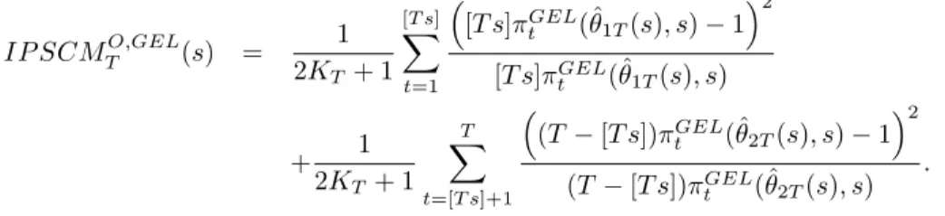
More precisely the statistic is defined as: IP SCTO,GEL(s) = 1 2KT + 1 [T s] X t=1 [T s]πtGEL(ˆθ1T(s), s)−1 2 (14) + 1 2KT + 1 T X t=[T s]+1 (T−[T s])πtGEL(ˆθ2T(s), s)−1 2 (15)
where ˆθ1T(s) = ˆβ1T(s) and ˆθ2T(s) = ˆβ2T(s). The statistic is the sum of the overidentifying restrictions statistics (10) but for the first and the second parts of the sample evaluated at the unrestricted estimator. The next Theorem establishes the asymptotic distribution of this statistic and the corresponding average mappings.
Theorem 4.4. Under Assumptions (7.1) to (7.10), the following processes indexed bys for a given set
S whose closure lies in (0,1) satisfy
IP SCTO,GEL(s)⇒Qq−r(s)
with under the null of no structural change
Qq−r(s)⇒
Bq−r(s)0Bq−r(s)
s +
[Bq−r(1)−Bq−r(s)]0[Bq−r(1)−Bq−r(s)] 1−s
and under the alternative (8)
Qq−r(s) ⇒ Bq−r(s)0Bq−r(s) s + H(s)0Ω−1/2(I−P G) Ω−1/2H(s) s [Bq−r(1)−Bq−r(s)]0[Bq−r(1)−Bq−r(s)] 1−s + [H(1)−H(s)]0Ω−1/2(I−P G) Ω−1/2[H(1)−H(s)] (1−s) ,
whereBq−r(s)is aq−r-vector of standard Brownian motion andPG =PGβ withPGβ = Ω −1/2G β G0βΩ−1G β −1 G0Ω−1/2. Moreover,
supIP SCTO,GEL⇒sup
s∈S
Qq−r(s), aveIP SCTO,GEL⇒
Z
S
Qq−r(s)dJ(s),
expIP SCTO,GEL⇒log
Z S exp[1 2Qq−r(s)]dJ(s) .
Proof: See the Appendix.
The Theorem shows that the proposed test statistics can detect instability occurring in overidentifying restrictions before and after the breakpoint. Indeed, the term H(s)0Ω−1/2(I−PG)Ω−1/2H(s)
s corresponds to a structural change in the moment conditions before the breakpointswhile the term
[H(1)−H(s)]0Ω−1/2(I−PG)Ω−1/2[H(1)−H(s)]
(1−s) to a structural change after the breakpoints.
The asymptotic critical values for the intervalS = [.15, .85] can be found in Hall and Sen (1999). For other symmetric interval [s0,1−s0], critical values can be obtained in Guay (2003), Tables 1 to 3 for a number of overidentifying restrictions divided by 2 (in those Tables). To see this, note that the critical
values for the supremum, the average and the log exponential mappings applied to B2q−2r(s)0B2q−2r(s)
s are
equivalent to ones corresponding to Bq−r(s)0Bq−r(s)
s +
(Bq−r(1)−Bq−r(s))0(Bq−r(1)−Bq−r(s))
1−s for a symmetric intervalS.4
An asymptotic equivalent statistic to (14) in the spirit of the Neyman-modified chi-square is given by:
IP SCMTO,GEL(s) = 1 2KT+ 1 [T s] X t=1 [T s]πGEL t (ˆθ1T(s), s)−1 2 [T s]πGEL t (ˆθ1T(s), s) + 1 2KT + 1 T X t=[T s]+1 (T−[T s])πGEL t (ˆθ2T(s), s)−1 2 (T−[T s])πGEL t (ˆθ2T(s), s) . 5 Simulation Evidence
To evaluate the performance of the test statistics we use the data generating process in Ghyselset al. (1997) and in Hall and Sen (1999). The time series model used is an AR(1) process for the variablext. One parameter is estimated, the autoregressive parameter (denoted byθin the expression below), using two moment conditions formed with the lagged values ofxt.
The data generating process is given by
xt=θixt−1+ut (16)
for t = 1, . . . , T. Structural change in the identifying restrictions (in the parameter) is studied by con-sidering different values ofθi where the indexi= 1,2 denotes the first or second subsamples. Structural stability in the overidentifying restrictions is studied by allowing for an ARMA(1,2) model
xt=θixt−1+ut+αut−2 (17)
and considering nonzero values of αin the second subsample. The change is set at T /2. In the above,
ut∼N(0,1). The sample size was set to 200 observations and the number of Monte Carlo replications was limited to 500 since the time required to estimate by exponential tilting, the method used in these simulations experiments.
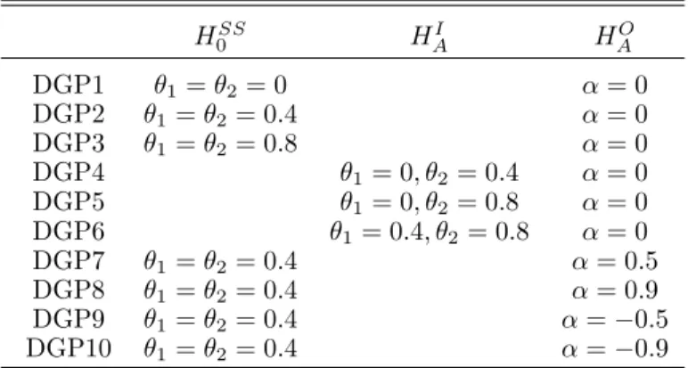
Table 7 summarizes the different parametrization and is taken from Hall and Sen (1999). The null hypothesis of structural stability is denoted byHSS
0 (DGP 1 to 3). For those DGPs we vary the magnitude of the autoregressive parameter θ. The alternatives of instability in the parameters or in the overidenti-fying restrictions are denoted by HAI (DGP 4 to 6), where we vary the magnitude of the change in the autoregressive parameter, andHAO (DGP 7 to 10) where we consider various values of the moving average
4This is verified by comparing the critical values in Hall and Sen (1999) and Guay (2003). The critical values in Table 1
parameter, respectively. In this situation only one parameter is estimated using two moment conditions created with the first two lags ofxt. UnderH0SS, whereα= 0, the instruments are appropriate. Under the first class of alternative hypothesis (HAI) the two instruments are also valid while they no longer are for the second part of the sample with the second class of alternative hypothesis (HAO).
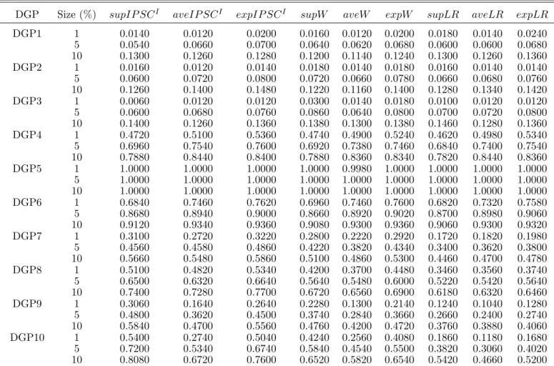
Smoothing the moment conditions is done via an appropriate choice of KT. In a GMM setting this is equivalent to using some form of estimate of the long run covariance matrix of the moment conditions (for example using the Newey-West estimator as the weight matrix in quadratic form). Most of the previous simulation work considered a fixed degree of smoothing (see for example Gregoryet al. (2002) and Guggenberger and Smith (2007)). Otsu (2006) did also look at fixed smoothing but also looked at applying the automatic bandwidth selection rule of Newey and West (1994).
Our Monte Carlo study is not specially designed to investigate smoothing because under the null hypothesis the optimal value of KT is 0 while it is not 0 under the alternative hypothesis HAO. For this reason we setKT = 0 for all DGPs except DGPs 7, 8, 9 and 10. For these DGPs we select a bandwidth parameter chosen via the automatic, data-driven, procedure which chooses a bandwidthmT which is then transformed as KT = [(mT −1)/2]. The average, taken over Monte Carlo replications, KT was found to vary between 1.6 and 2.3, increasing with the moving average component. A complete analysis of the effects of smoothing is left for future work. Lastly, a trimming rule of 0.15 was used, namelyS= [.15, .85]. Table 5 contains the results for the general specification tests IP SC and IP SCM (the supremum, exponential and average version of the test statistics are presented). Table 6 contains the rejection fre-quencies for the test statistics designed to have power against a structural change in the parameters while Table 7 presents the results for test statistics which are designed to have power against a structural change in the overidentifying restrictions. All the test statistics were all computed in the GEL setting. The tests used for comparison appear in Guay and Lamarche (2008). For completeness we report them also here: W aldT(s) =T ˆ β1T(s)−βˆ2T(s) 0 ( ˆVΩ(s))−1 ˆ β1T(s)−βˆ2T(s) , where ˆVΩ(s) = ˆ V1(s)/s+ ˆV2(s)/(1−s) and ˆVi(s) = ˆ Gβi,tT(s)0Ωˆi,T−1(s) ˆGβi(s) −1 fori= 1,2 correspond-ing to the first and the second part of the sample. For the first part of the sample:
ˆ Gβ1,tT(s) = 1 [T s] [T s] X t=1 ∂gtT( ˆβ1(s),δˆ(s)) ∂β01 b Ω1T(s) = 2KT + 1 [T s] [T s] X t=1 gtT(β1(s), δ)gtT( ˆβ1(s),δˆ(s))0
and for the second part of the sample: b Gβ2,tT = 1 T−[T s] T X t=[T s]+1 ∂gtT( ˆβ2(s),δˆ(s)) ∂β20 b Ω2T(s) = 2KT + 1 T−[T s] T X t=[T s]+1 gtT( ˆβ2(s),δˆ(s))gtT( ˆβ2(s),δˆ(s))0.
The Lagrange Multiplier statistic is given by:
LMT(s) = T s(1−s)g1T(˜θT, s) 0Ωˆ−1 T Gˆ β tT h ( ˆGβtT)0Ωˆ−T1GˆβtTi −1 ( ˆGβtT)0ΩˆT−1g1T(˜θT, s). where g1T(˜θT, s) = 1 T [T s] X t=1 gtT(˜θT), ˆ GβtT = 1 T T X t=1 ∂gtT( ˜β,˜δ) ∂β0 , b ΩT = 2KT + 1 T T X t=1 gtT( ˜β,˜δ)gtT( ˜β,δ˜)0. The LR-like statistic is defined as:
LRT(s) = 2T 2K+ 1 T X t=1 h ρ(˜γ(s)0gtT(˜θ, s))−ρ0 i T − T X t=1 h ρ(ˆγ(s)0gtT(ˆθ(s), s))−ρ0 i T
An finally, the test statistic proposed by Hall and Sen (1999) is
OT(s) =O1T(s) +O2T(s) where O1T(s) = 1 p [T s] [T s] X t=1 gtT( ˆβ1(s),δˆ(s)) 0 ˆ Ω−1T1(s) 1 p [T s] [T s] X t=1 gtT( ˆβ1(s),ˆδ(s)) and O2T(s) = 1 p (T−[T s]) [T] X t=[T s]+1 gtT( ˆβ2(s),δˆ(s)) 0 ˆ Ω−2T1(s) 1 p (T−[T s]) X t=[T s]+1 gtT( ˆβ2(s),ˆδ(s))
Focusing first on size we find that the modified tests (IP SCM1I,IP SCM2I andIP SCMO) based on implied probabilities have rejection frequencies that are much too large. The intuition for this is that the modified test statistics contain a more volatile term in the denominator which can inflate the value of the tests and hence increase the rejection frequencies. So for brevity, we don’t report those results here.5
On the other hand, all other tests have rejection frequencies that are quite good, with some overrejec-tion except for theO test statistics which slightly underreject . The supIP SCI has a nominal size close to the true one while the average and exponential forms for this statistic slightly overreject, a property shared by theW aldandLRtests. TheLMtest statistics (supremum, average and exponential mappings) significantly underreject for all DGPs (1 to 3) under the null and have poor power for other DGPs. For these reasons, the rejection frequencies for theLM test statistics are not reported in the tables here.
The study of power is divided into two cases. In case 1 structural change occurs in the parameter values while in case 2 structural change occurs in the overidentifying restrictions. Under the alternative of instability in the parameter,HI
A(DGP 4 to 6), we see that the newly proposed test statistics based on implied probabilities have good rejection frequencies. The power of these test statistics is equal or larger than the power of the standard W ald andLR tests. TheIP SCO and O test statistics, geared toward instability in the overidentifying restrictions, have not useful power while the more general specification test,IP SC, has some reasonable power.
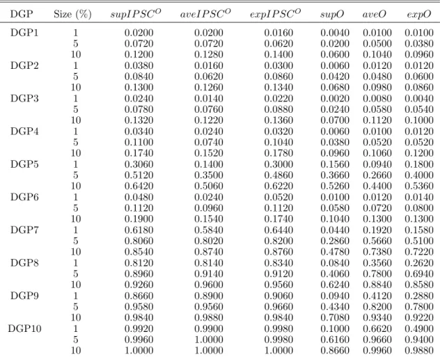
Under the alternative of instability in the overidentifying restrictions, e.g.HO
A, (DGP 7 to 10), we see that the test statistics specially designed to detect a change in the parameterIP SCI, and the standard
W ald and LR tests have little power while the targeted IP SCO and O tests have very good power.
Importantly the tests based on implied probabilities are seen to have significantly higher power than O
tests for all cases. In some cases, the gain in power can be twice as important. As expected, the general specification tests based on implied probabilities have rejection frequencies that fall between those of
IP SCO andIP SCI.
The increase in the autoregressive coefficient from 0 to 0.8 does not impact greatly on the rejection frequencies under the null hypothesis but under the alternative hypotheses the magnitude of the change is important. UnderHI
A, for example, we see that power is close to unity when the change in the autore-gressive parameter is quite extreme (0 to 0.8). UnderHO
A, which captures a change in the overidentifying restrictions, an increase (in absolute terms) in the moving average coefficient increases power.
6 Conclusion
As noted by Back and Brown (1993) implied probabilities obtained from estimation of models using estimating equations could be used as an additional tool for model specification in the researcher’s tool kit. An important specification test that has received considerable attention in the econometric literature has been a test for structural stability of either the underlying key parameters composing the estimation equations and or the stability of the additional equations (the overidentifying restrictions) that are often used in estimation. In this paper we have focused on the class of estimators based on the Generalized Empirical Likelihood approach. This approach is appealing intuitively because it requires the search for a
vector of weights, one for each observation, that yields the most probable data distribution. We view these weights as potentially containing information on the content of the moment conditions (the estimating equations). In a pure entropy setting with no estimating equations the vector of weights is found to be maximally uninformative. That is we obtain weights fluctuating around 1/T whereT is the sample size. With constrains, the weights are chosen to be as maximally uninformative as the constraints will allow.
In this sense the weights make use of the available information contained in the sample. In particular we use the weights to detect an unknown structural change. We suggest three types of testing procedures for the detection of a structural change each based on different measures of the discrepancy between the estimated weights and the unconstrained weights T1. Specifically, we propose general structural change tests to detect instability both in the identifying restrictions and in the overidentifying restrictions, instability in the identifying restrictions and finally instability in the overidentifying restrictions. This type of classification is similar to the one found in classical papers on structural change in time series as proposed by Andrews (1993) and Hall and Sen (1999) for example. We found that tests based on these implied probabilities have good finite sample size and power properties. An issue that was not investigated in length in this paper was the impact of smoothing (to take into account serial dependence) on the performance of the tests. This interesting avenue of research is left for future work. The important question of structural change tests for GEL robust to weak identification is also left for future investigation.
7 Appendix 7.1 Assumptions
Assumption7.1. The process{xt}∞t=1is a finite dimensional stationary and strong mixing coefficients P∞
j=1α(j) (ν−1)/ν
< ∞for someν >1.
Assumption 7.2. (a) (β0, δ0)∈ B×∆is the unique solution to E[g(xt, β, δ)] = 0 where B×∆is compact,
g(xt, β, δ)is continuous at each(β, δ)∈B×∆with probability one;(b)E h
sup(β,δ)∈B×∆kg(xt, β, δ)kα i
<∞for someα >max“4ν,1η”;(c)Ω(β, δ) is finite and positive definite for all(β, δ)∈B×∆.
Define the smoothed moment conditions as: gtT(β, δ) = 1 S t−1 X s=t−T k „ s ST « gt−s(xt, β, δ)
for an appropriate kernel. From now on, we consider the uniform kernel proposed by Kitamura and Stutzer (1997):
gtT(β, δ) = 1 2KT+ 1 KT X s=−KT gt−s(xt, β, δ) Assumption7.3. KT2/T→0andKT → ∞asT → ∞.
Assumption 7.4. (a) ρ(·) is twice continuously differential and concave on its domain, an open interval Φ
containing 0,ρ1=ρ2=−1;(b)γ∈ΓwhereΓ ={γ:kγk ≤D `
T /KT2 ´−ζ
}for some D >0with 12 > ζ > 2αη1 .
Under Assumptions 7.1 to 7.4, Smith (2004) shows that for the full-sample estimators ˜θT p → θ0, ˜ γT p → 0, kγ˜Tk = Op T /2KT+ 1)2 −1/2 and k1 T PT t=1gtT(˜θT)k = Op(T−1/2). Now, Let G(β, δ) = E[∂g(xt, β, δ)/∂(β0, δ0)] andG=G(β0, δ0).
Assumption 7.5. g(·, β, δ) is differentiable in (β0, δ0)∈B0×∆0 where B0×∆0 is a neighborhood of (β0, δ0),sup1≤t≤TE
h
sup(β,δ)∈B
0×∆0k∂g(xt, β, δ)/∂(β
0, δ0)kα/(α−1)i<∞ andrank(G) =p+ν. Assumptions 7.1 to 7.5 yield the asymptotic distribution ofT1/2θ˜T −θ0and T /(2KT + 1)21/2
˜
γT (see Smith, 2004). Also, under these assumptions:
1 T T X t=1 GtT( ˜βT,δ˜T) p →G and ˜ ΩT(˜θT) = 2K+ 1 T T X t=1 gtT( ˜βT,δ˜T)gtT( ˜βT,δ˜T)0 p →Ω.
The following high level assumptions are sufficient to derive the weak convergence under the null of the PS-GEL estimators ˆθT(s) and ˆγT(s) (see Guay and Lamarche, 2008). These assumptions are similar to the ones in Andrews (1993).
Assumption 7.6. V ar√1 T
PT s
t=1g(xt, θ)
→sΩ ∀s∈[0,1] for some positive definite matrix Ωwhere
Ω = limT→∞V ar 1 √ T PT t=1g(xt, θ) .
Assumption 7.7. sups∈SkΩˆT(s)−Ω(s)k p
→0 whereΩ(s)is defined in Section 3.1 andS whose closure lies in(0,1).
Assumption 7.8. sups∈SkθˆT(s)−θ0k p
→0 for someθ0in the interior ofΘandsups∈SkγˆT(s)−0k p →0
andS whose closure lies in (0,1). Assumption 7.9. limT→∞T1
PT s
t=1E∂g(xt, β0, δ0)/∂(β0, δ0)exists uniformly over s∈S and equals sG ∀s∈S andS whose closure lies in (0,1).
Assumption 7.10. G(s)0Ω(s)−1G(s)is nonsingular∀s∈Sand has eigenvalues bounded away from zero ∀s∈S andS whose closure lies in (0,1).
7.2 Lemmas
The following Lemmas are necessary to establish the proofs of the Theorems:
Lemma 7.1. We denote{B(s) :s∈[0,1]} asq-dimensional vectors of mutually independent Brownian motion on[0,1]and define
J(s) =
Ω1/2B(s) Ω1/2(B(1)−B(s))
where B(π) is a q-dimensional vector of standard Brownian motion. Under Assumptions 7.1 to 7.10, every sequence of PS-GEL estimators{θˆ(·),γˆ(·), T ≥1} satisfies
√ TθˆT(·)−θ0 ⇒ − G(·)0Ω(·)−1G(·)−1G(·)0Ω(·)−1J(·), √ T 2KT+ 1 ˆ γT(·) ⇒ − Ω(·)−1−Ω(·)−1 G(·)0Ω(·)−1G(·)−1 G(·)0Ω(·)−1J(·)
as a process indexed bys∈S, whereS has closure in (0,1). Further, the sequence GEL estimatorsθˆT(·)
and the sequence of auxiliary estimatorsγˆT(·)are asymptotically uncorrelated. Under the alternative (8),
the same results hold except that:
J(s) = Ω1/2B(s) +H(s) Ω1/2(B(1)−B(s)) +H(1)−H(s) whereH(s) =Rs
0 h(r)drwithh(r) =h(η, τ, r)to simplify the notation.
Proof of Lemma 7.1: see Guay and Lamarche (2008).
Lemma 7.2. Under Assumptions 7.1 to 7.10, for the unrestricted implied probabilities evaluated at the restricted estimator, we get
πtGEL(˜θT, s) = 1 T + 1 TgtT(˜θT, s) 0 e γT(s)(1 +op(1)) +Op KT/T2
and πGELt (˜θT) = T1 +op(1) uniformly in t = 1, . . . , T. According to notation in Definition 3.4, for
t= 1, . . . ,[T s],
T πtGEL(˜θT, s)−1 =gtT( ˜βT,δ˜T)0eγ1T(1 +op(1)) +Op(KT/T)
and fort= [T s] + 1, . . . , T,
Proof of Lemma 7.2
We need to derive the asymptotic distributions of the partial-sample implied probabilities evaluated at the full-sample estimator, namely:
πGELt (˜θT, s) = ρ1 e γT(s)0gtT(θeT, s) PT t=1ρ1 e γT(s)0gtT(eθT, s) .
A mean value expansion forπGEL
t (˜θT, s) around (˜θT,γ˜T) = (˜θT,0) yields: πGELt (˜θT, s) = 1 T + ρ2 ¯ γT(s)0gtT(eθT, s) PT t=1ρ1 e γT(s)0gtT(θeT, s) gtT(θeT, s) 0 e γT(s)− ρ1 e γT(s)0gtT(θeT, s) h PT t=1ρ1 ¯ γT(s)0gtT(θeT, s) i2 T X t=1 ρ2 ¯ γT(s)0gtT(θeT, s) gtT(θeT, s)0eγT(s)
where ¯γT(s) lies on the line segment joiningeγT(s) and 0 and may differ from row to row.
Since ˜γT(s) converges in probability to 0 and using Lemma A.4 in Smith (2004), this yields that
ρj
¯
γT(s)0gtT(θeT, s)
=ρj(0) +op(1) =−1 +op(1), forj= 1,2,∀t. Thus, we get:
πGELt (˜θT, s) = 1 T + 1 T h gtT(˜θT, s)0eγT(s) (1 +op(1)) i − 1 T2 " T X t=1 gtT(˜θT, s)0eγT(s) (1 +op(1)) # . As PT t=1g(˜θT) = PT t=1gtT(˜θT) +Op K 2/(2K+ 1) = Op(T1/2) which implies PTt=1gtT(˜θT, s) = Op(T1/2),gtT(˜θT, s) =Op((2KT + 1)−1/2) and ˜γT(s) =Op(2KT + 1/ √ T)6yields: πGELt (˜θT, s) = 1 T + 1 T h gtT(˜θT, s)0γ˜T(s) (1 +op(1)) i +Op KT/T2 and πGELt (˜θT, s) = 1 T (1 +op(1)).
uniformly int= 1, . . . , T. Thus, we get:
T πGELt (˜θT, s)−1 =gtT( ˜βT,˜δT)0˜γ1T(1 +op(1)) +Op(KT/T). (18) uniformly int= 1, . . . ,[T s] and
T πGELt (˜θT, s)−1 =gtT( ˜βT,˜δT)0˜γ2T(1 +op(1)) +Op(KT/T). (19) uniformly int= [T s] + 1, . . . , T.
7.3 Proofs of Theorems
Proof of Theorem 4.1
We expand the FOC of the Lagrange multiplier vector for the partial-sample GEL evaluated at the restricted estimator in a Taylor series about 0 for the first part of the samplet= 1, . . . ,[T s]. Thus
1 T [T s] X t=1 ρ1 ˜ γ01TgtT( ˜βT,δ˜T) gtT( ˜βT,δ˜T) = − 1 T [T s] X t=1 gtT( ˜βT,δ˜T)− 1 T [T s] X t=1 gtT( ˜βT,δ˜T)gtT( ˜βT,δ˜T)0γ˜1T + 1 T [T s] X t=1 gtT( ˜βT,˜δT) ∞ X j=2 1 j!ρj+1(0) gtT( ˜βT,δ˜T)0γ˜1T j
where ˜γ1T is the partial-sample Lagrange multiplier evaluated for the restricted estimator for t = 1, . . . ,[T s] andρ1(0) =ρ2(0) =−1. By the fact thatgtT( ˜βT,δ˜T) =Op (2KT + 1)−1/2
, this yields 1 T [T s] X t=1 ρ1 ˜ γ01TgtT( ˜βT,δ˜T) gtT( ˜βT,δ˜T) = − 1 T [T s] X t=1 gtT( ˜βT,δ˜T)− 1 T [T s] X t=1 gtT( ˜βT,δ˜T)gtT( ˜βT,δ˜T)0γ˜1T + Op (2KT + 1)−3/2k˜γ1Tk2 .
By using a consistent estimator ˜ΩT = 2[KT s+1] P [T s] t=1gtT( ˜βT,δ˜T)gtT( ˜βT,˜δT)0and ˜γ1T =Op (2KT + 1)/ √ T, we get under the null:
0 = 1 T [T s] X t=1 gtT( ˜βT,˜δT) + s 2K+ 1 ˜ ΩT˜γ1T +Op (2KT+ 1)−3/2kγ˜1Tk2 which yields s 2KT+ 1 ˜ γ1T =−Ω˜−T1 1 T [T s] X t=1 gtT( ˜βT,δ˜T) +Op KT1/2/T. (20)
Now, expanding this expression aroundβ0 andδ0gives:
s√T 2KT+ 1 ˜ γ1T =−Ω˜−T1 1 √ T [T s] X t=1 gtT(β0, δ0)−sΩ˜−T1G √ T ˜ βT −β0 ˜ δT −δ0 +op(1).
We can easily show for the restricted estimators under the null that (see also Smith, 2004): √ T ˜ βT −β0 ˜ δT −δ0 =− G0Ω−1G−1 G0Ω−1√1 T T X t=1 gtT(β0, δ0) +op(1). (21)
Combining the two preceding results, we obtain
s√T 2KT + 1 ˜ γ1T = −Ω−1 1 √ T [T s] X t=1 gtT(β0, δ0) +sΩ−1G(G0Ω−1G)−1G0Ω−1 1 √ T T X t=1 gtT(β0, δ0) +op (1).