SPC-based Inventory Control Policy to Improve Supply Chain Dynamics

SPC-based Inventory Control Policy to

Im-prove Supply Chain Dynamics

Francesco Costantino#1, Giulio Di Gravio#2, Ahmed Shaban#3,*, Massimo Tronci#4

#

via Eudossiana 18, 00184 Rome, Italy

Department of Mechanical and Aerospace Engineering, University of Rome “La Sapienza”, *Department of Industrial Engineering, Faculty of Engineering, Fayoum University, Fayoum 63514, Egypt

1 [email protected] 2 [email protected] 3 [email protected] 4

Abstract—Inventory control policies have been recognized as a contributory factor to the bullwhip effect and inventory instability. Previous studies have indicated that there is a trade-off between bullwhip effect and inventory performance where the bullwhip effect reduction might increase inventory instability. Therefore, there is a need for inventory control policies that can cope with supply chain dynamics. This paper proposes an inventory control policy based on a statistical process control approach (SPC) to handle supply chain dynamics. The policy relies on applying individual control charts to control both the inventory position and the placed orders adequately. A simulation study has been conducted to evaluate and compare the proposed SPC policy with a traditional order-up-to in a multi-echelon supply chain. The comparison showed that the SPC policy outperforms the order-up-to in terms of bullwhip effect and inventory performances. The SPC succeeded to eliminate the bullwhip effect whilst keeping a competitive inventory performance.

massimo.tronci @uniroma1.it

Keyword—Supply Chain, Inventory Control, SPC, Control Chart, Bullwhip Effect, Inventory Variance, Si-mulation

I. INTRODUCTION

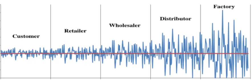
In supply chains, the variability in the ordering patterns often increases as demand information moves up-stream in the supply chain, from the retailer towards the factory and the suppliers. This phenomenon of informa-tion distorinforma-tion has been recognized as the bullwhip effect [1]. Fig. 1 depicts an example of the bullwhip effect in which the orders placed by four supply chain echelons over the same 100 periods are plotted side-by-side. The bullwhip effect has been observed in many industries such as Campbell Soup’s [2], HP and Proctor & Gamble [1], fast moving consumer goods [3], and car manufacturing [4]. Forrester [5] was mostly the first to study this problem through a set of simulation experiments using system dynamics approach. Another number of research-ers developed simulation games to illustrate the bullwhip effect existence and its negative impacts on supply chain performance [6]. Towill, Zhou, and Disney [7] indicated that the bullwhip effect could lead to stock-outs, large and expensive capacity utilization swings, lower quality products, and considerable production/transport on-costs as deliveries are ramped up and down at the whim of the supply chain [8], [9].

Lee, Padmanabhan, and Whang [1] identified five fundamental causes of bullwhip effect: demand signal processing, non-zero lead-time, order batching, price fluctuations and rationing and shortage gaming. Under demand signal processing, demand is forecasted using a forecasting method, and then the parameters of the in-ventory replenishment rules are updated in accordance to demand changes. By doing this, the system may over react to short-run fluctuations, which induces variance amplification [10]. Burbidge’s Law of Industrial Dynics states that ‘If demand is transmitted along a series of inventories using stock control ordering, then the am-plitude of demand variation will increase with each transfer’ [11]. Thus, inventory management decisions can be considered as a main driver of bullwhip effect and can be classified under the demand signal processing cause [10]. However, inventory managers must consider two primary factors when making inventory replenishments [12]. First, a replenishment rule has an impact on order variability (as measured by the bullwhip effect, i.e., the ratio of the variance of orders over the variance of demand) shown to the supplier (see Fig. 1). Second, the re-plenishment rule has an impact on the variance of the net stock (as measured by the net stock amplification, i.e., the ratio of net stock variance over the variance of demand). The bullwhip effect mainly contributes to upstream costs, while the variance of net stock determines the stage’s ability to meet a service level in a cost-effective manner. This trade-off needs designing a good replenishment rule to balance the inventory and production costs whilst ensuring a customer service level [12]. Exhaustive research has been conducted to study the impact of various ordering policies on bullwhip effect and other research has also attempted to develop ordering and re-plenishment rules that can avoid the creation of bullwhip effect [13]-[19].

0 10 20 30 40 50 60 70 80 90 0 100 200 300 400 500 O rde r quan ti ty Customer Retailer Wholesaler Distributor Factory

Fig. 1. An example of demand amplification (bullwhip effect).

The trade-off between bullwhip effect and inventory performance is still a major concern for both supply chain managers and academics. The practitioners need a simple ordering policy that can handle this trade-off without major implementation effort [13]. The ordering policies should also be smart enough to monitor its in-ternal and exin-ternal environments and making the appropriate changes whenever it is needed.

Recently, a few number of researchers have introduced the Statistical Process Control (SPC) tools in the area of inventory planning and control. Watts et al. [20] was mostly the first to present a control chart approach for monitoring the performance of a reorder-point inventory system through monitoring stock-outs and applying control charts for demand and inventory turnover to identify whether the causes of system malfunctions related to system fitness or ongoing operations. Pfohl, Cullmann, and Stölzle [21] developed a real-time inventory deci-sion support system by using the traditional Shewhart control charts for inventory level and demand in which a series of decision rules are provided to help the inventory manager to determine the time and the quantity to or-der. They argued that the proposed inventory decision system showed very good results where the average in-ventory levels could have been reduced by 20% to 65% which might save inin-ventory costs. Cheng and Chou [22] extended the work of Pfohl, et al. and introduced an inventory decision system in which the ARMA control chart was employed to monitor the market demand and the individual control chart with western electric rules was used to monitor the inventory level. Lee and Wu [23] compared two replenishment approaches, namely, traditional replenishment policies and statistical process control SPC-based replenishment policy. They con-cluded that SPC-based policy had shown better reduction of inventory variability than the traditional methods. With exception to Lee and Wu [23] who adopted a two-echelon supply chain to compare a SPC policy with the traditional policies, the majority of the above SPC work considered a single echelon supply chain in order to evaluate the effectiveness of SPC ordering policies. Also, some of those authors neglected the effect of lead-time in their inventory models. Furthermore, the performance measures that have been used in the previous work to evaluate those inventory models did not consider the supply chain dynamics such as bullwhip effect ra-tio and inventory variance. The common measures in their studies were service level and average inventory level. In this study, we will be more interested in the dynamic performance of the supply chain under ordering policies.

This research considers the previous attempts to utilize SPC control charts for inventory control. In particular, this work proposes a new inventory control policy based on SPC control charts to be used in dynamic and com-plex environments like multi-echelon supply chains. The main objective of the SPC policy is to overcome the dynamic problems of the traditional inventory management systems through controlling mainly the problem of demand variability amplification whilst managing simultaneously the inventory position. A simulation approach is adopted to conduct the study and to evaluate the performance of a multi-echelon supply chain under the pro-posed SPC policy. Furthermore, a comparison will be conducted between the SPC policy and the traditional or-der-up-to ordering policy in terms mainly of bullwhip effect, inventory stability and service level. The simula-tion result showed that the SPC performs better than the tradisimula-tional order-up-to policy where SPC succeeded to eliminate the bullwhip effect whist achieving a satisfactory inventory performance.

II. SPCREPLENISHMENT POLICY

The proposed SPC replenishment policy is an integrated inventory control system that can monitor the inven-tory position and place balanced orders to the upstream echelons in the supply chain. The main idea is that us-ing a control chart to establish a statistically valid zone, defined by upper and lower control limits instead of single point replenishment, would allow dampening the overreactions that can cause the bullwhip effect and in-ventory variance amplification.

The SPC replenishment policy relies on two control charts to be used for monitoring demand and inventory position simultaneously. The first control chart is devoted to monitor the variation of the customer demand over time so that the appropriate changes in the ordering behavior can be made whenever a considerable change in the demand has been detected. In other words, if the customer demand is stable (i.e., in-control), then the order quantity will be the same as ever before. However, if the demand control chart signals the presence of an out-of-control situation (i.e., demand change), then the order quantity should be adjusted in order to account for the

in-ventory stability. Accordingly, the demand control chart should be complemented with a number of decision rules in order to decide about the out-of-control situation and how much to order under different out-of-control situations. The base order quantity will then be added to the required adjustment for the inventory position in order to constitute the final order to place.

The second control chart is employed for monitoring and adjusting the inventory position whenever it is needed. This control chart will be employed to identify whether the inventory position variable is in-control or not. This control chart is complemented with a number of decision rules to adjust the inventory position when-ever it is needed. For example, if the current data point of inventory position is very low, then a decision rule will be needed to detect this situation and propose an amount of adjustment to be added to the base order quan-tity.

A. Control Charts and Decision Rules

The type of control chart that will be used for both demand and inventory position is called the individual control chart in which the sample size is equal to one. A typical control chart consists of three basic elements: centerline that represents the average of the process variable, and upper and lower control limits [24]. Based on the normality assumption, it is expected that 99.73% of the demand data points will be within the lower and up-per control limits if a process variable (e.g., customer demand process) is in-control. The control limits of the demand and inventory position control charts can be calculated as follows in Table I.

Table I

Control Charts Calculations

Demand Control Chart Inventory Position Control Chart

ˆ 3 i i i D D D UCL =CL + σ UCLiIP=CLiIP+3σˆIPi 1 1 i t i t D i t w i CL D w − + =

∑

In the above table, the i

D

CL represents the centerline of the demand/incoming order control chart and is

cal-culated based on the average of the last consecutive wi data points of the incoming order data. The

i D LCL

represents the lower control limit and equals the difference between i

D CL and 3ˆi D σ where ˆi D σ is the standard

deviation of the demand variable over the last consecutive wi data points. The upper control limit (

i D UCL )

equals the sum of i

D

CL and 3ˆi

D

σ . The centerline of the inventory position control chart is equal to i

D

CL

multi-plied by the delivery lead-time ( i

d

L ) and added to the safety stock component. Alternatively, we extend the

de-livery lead-time with ki to account for the safety stock.

The decision rules corresponding to the demand control chart will be dependent on the status of the last ob-servations of the incoming order as they are the most important information for managing the ordering process. This is similar to the traditional policies in which the ordering process is driven by a forecasting technique that usually relies on the latest information to make expectations for the future demand.

B. Base Order Quantity

At echelon i, if the last consecutive ni data points of incoming order/demand are either above or below a

de-fined safety zone between i i ˆi

D D D

CL −K σ and i i ˆi

D D D

CL +K σ , then the base order quantity (Oti) should be set as

follows in equation (1). However, if this condition is not satisfied, then the base order quantity should be equal to the centerline of the demand control chart as follows in equation (2). In case of the demand or the incoming

order to echelon i is zero, then, the order quantity of echelon i should be set to zero (i.e., i 0

t O = ). 1 1 i t i i t t t n i O IO n − + =

∑

∑

At echelon i, if the last observation on the inventory position control chart, i t

IP , is above the upper limit of a

safety zone ( i i i

IP IP IP

CL +K σ ), then, a negative inventory balance should be added to the base order quantity. This

inventory balance ( i

t

Invb ) can be calculated as follows in equation (3):

i i i i i

t IP IP IP t

Invb =CL +K σ −IP (3)

Otherwise, if the last observation on the inventory position control chart, i

t

IP , is below the lower limit of a

safety zone ( i i i

IP IP IP

CL −K σ ), then, a positive inventory balance should be added to the base order quantity (see,

equation (4)).

i i i i i

t IP IP IP t

Invb =CL −K σ −IP (4)

Finally, if the last observation is within the safety zone (i.e., i i i i i i i

IP IP IP t IP IP IP

CL −K σ ≤IP ≤CL +K σ ), then, there

is no need for inventory balance, i.e., i 0

t Invb = .

The final order that should be placed at the end of review time t will be equal to the sum of the base order

quantity and the inventory balance as shown in equation (5):

{ , 0}

i i i

t t t

O =Max O +Invb (5)

III. SUPPLY CHAIN MODELING AND SIMULATION

A. Supply Chain Model and Assumptions

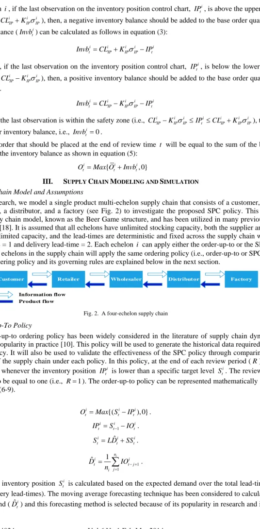
In this research, we model a single product multi-echelon supply chain that consists of a customer, a retailer, a wholesaler, a distributor, and a factory (see Fig. 2) to investigate the proposed SPC policy. This is a well-known supply chain model, well-known as the Beer Game structure, and has been utilized in many previous investi-gations [16]-[18]. It is assumed that all echelons have unlimited stocking capacity, both the supplier and the fac-tory have unlimited capacity, and the lead-times are deterministic and fixed across the supply chain with

order-ing lead-time = 1 and delivery lead-time = 2. Each echelon i can apply either the order-up-to or the SPC policy.

However, all echelons in the supply chain will apply the same ordering policy (i.e., order-up-to or SPC). The or-der-up-to ordering policy and its governing rules are explained below in the next section.

Retailer Wholesaler Dis tributor Factory

Customer

Information flow Product flow

Fig. 2. A four-echelon supply chain B. Order-Up-To Policy

The order-up-to ordering policy has been widely considered in the literature of supply chain dynamics be-cause of its popularity in practice [10]. This policy will be used to generate the historical data required to initiate the SPC policy. It will also be used to validate the effectiveness of the SPC policy through comparing the

per-formances of the supply chain under each policy. In this policy, at the end of each review period (R), an order

i t

O is placed whenever the inventory position i

t

IP is lower than a specific target level i

t

S . The review period is

considered to be equal to one (i.e., R=1). The order-up-to policy can be represented mathematically as follows

in equations (6-9). {( ), 0} i i i t t t O =Max S −IP . (6) 1 i i i t t t IP =S₋ −IO . (7) ˆ i i i t t t S =LD +SS . (8) 1 1 1 ˆi ni i t t j j i D IO n = − + =

∑

The target inventory position i

t

S is calculated based on the expected demand over the total lead-time

(order-ing and delivery lead-times). The mov(order-ing average forecast(order-ing technique has been considered to calculate the

as well [10], [14]. In this model, we have considered the safety stock by extending the lead-time by ki [16],

[18], [25] so that the target inventory position Sti can thus be reformulated as shown below in equation (10).

This is similar to what we have done with the centerline of the inventory position control chart. ˆ ( ) i i t i t S = L+k D (10) C. Performance Measures

The performance of the supply chain under the proposed SPC and OUT policy will be evaluated through characterizing the ordering and inventory behavior under each policy throughout the whole supply chain. The ordering behavior will be evaluated by estimating the following performance measures: average order level,

to-tal variance amplification or bullwhip effect (TVAi), and stage variance amplification (SVAi). The TVAi and

i

SVA are used to quantify the demand amplification throughout the supply chain. The TVAi, as shown in

equa-tion (11), is estimated in terms of the ratio of orders variance divided by the corresponding orders average at

echelon i to the customer demand variance divided by the average demand [10], [14], [18].

2 2 / / i i O O i D D TVA σ µ σ µ = (11)

The SVAi is estimated by comparing the order variance at echelon i to the order variance at echelon i−1;

each is divided by the corresponding mean as shown in equation (12) [26].

1 1 2 2 / / i i i i O O i O O SVA σ µ σ µ − − = ₍₁₂₎

The inventory behavior will be evaluated through estimating the following performance measures: average net inventory, inventory variance ratio, and average service level. The inventory variance ratio represents the

ra-tio of the actual net inventor variance ( 2

i

NI

σ ) to the customer demand variance as shown in equation (13) [27].

2 2 i NI i D InvR σ σ = (13)

The average service level quantifies the percentage of items delivered immediately by echelon i to the

in-coming order from echelon i−1. Service level or fill rate is computed every review time R over the effective

delivery time (i.e., i 0

t

IO > ) as shown in equation (14), where i

t

SR stands for the shipment from echelon i to

echelon i−1 at t, 1

i t

B₋ stands for the initial backlog at echelon i at t, i

t

IO is the incoming order to echelon i

at time t, and Teff stands for the effective delivery time.

1 1 1 100 0 0 0 i i i i t t t t i i t t i i t t SR B if SR B IO Sl if SR B − − −  − × − >  =   _{− ≤}  (14) 1 eff T _i t t i eff Sl ASl T = =

∑

IV. SIMULATION RESULTS AND ANALYSIS

A simulation model has been developed for the supply chain described above using SIMUL8 simulation package. To evaluate the proposed policy, the simulation model was run for 10 replications of 2400 periods each. Each simulation run consists of four stages, the first stage is a warm-up period for the order-up-to policy, and the second stage is the effective simulation run that the performance of the order-up-to will be collected over it. Then, another warm-period for the SPC policy is considered, followed by an effective simulation run for the SPC to collect the supply chain performance for the analysis. Both warm-up periods are set to be of the same length (i.e., 200 periods), and both effective simulation runs are set to be of the same length (i.e., 1000 periods). The warm-up period has been determined based on a set of preliminary experiments, and the numbers of repli-cations are based on a calculator tool in SIMUL8. This tool continues to run replirepli-cations until a confidence in-terval with a specified level (95%) and precision (15%) is obtained for a set of a predetermined performance measures.

The customer demand pattern was assumed to follow the normal distribution with a mean of 30 and a

stan-dard deviation of 3. The parameters of the order-up-to are set to ki =1, and mi =100, and the SPC policy

pa-rameters are set towi =100, 0.25

i IP

K = , i 1.5

D

K = , and ni =4. Furthermore, for simplicity, we set ˆ ˆ

i i

IP D

σ =σ

in all the following simulation experiments. A. Ordering Behavior

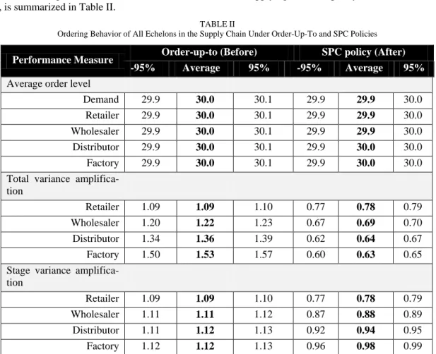
The ordering behavior of the supply chain in terms of average order level, total variance amplification, and stage variance amplification at each echelon, before and after applying the SPC policy, with 95% confidence level, is summarized in Table II.

TABLE II

Ordering Behavior of All Echelons in the Supply Chain Under Order-Up-To and SPC Policies

Performance Measure Order-up-to (Before) SPC policy (After)

-95% Average 95% -95% Average 95%

Average order level

Demand 29.9 30.0 30.1 29.9 29.9 30.0

Retailer 29.9 30.0 30.1 29.9 29.9 30.0

Wholesaler 29.9 30.0 30.1 29.9 29.9 30.0

Distributor 29.9 30.0 30.1 29.9 30.0 30.0

Factory 29.9 30.0 30.1 29.9 30.0 30.0

Total variance

amplifica-tion

Retailer 1.09 1.09 1.10 0.77 0.78 0.79

Wholesaler 1.20 1.22 1.23 0.67 0.69 0.70

Distributor 1.34 1.36 1.39 0.62 0.64 0.67

Factory 1.50 1.53 1.57 0.60 0.63 0.65

Stage variance

amplifica-tion

Retailer 1.09 1.09 1.10 0.77 0.78 0.79

Wholesaler 1.11 1.11 1.12 0.87 0.88 0.89

Distributor 1.11 1.12 1.13 0.92 0.94 0.95

Factory 1.12 1.12 1.13 0.96 0.98 0.99

Although we have selected a set of parameters for the order-up-to policy that was sufficient to reduce the bullwhip effect to a great extent, the results show that the order-up-to policy is still generating the bullwhip ef-fect and it is increasing as we move upstream from the retailer to the factory. In contrast, the SPC policy was successful to eliminate the bullwhip effect where the total variance amplification at all echelons (i.e., throughout the supply chain) is less than one. It can also be observed that the bullwhip effect under the SPC is decreasing as orders moves upstream in the supply chain. This can also be explained by the stage variance amplification that has a value lower than one at all echelons which means that each echelon is acting as a filter for the incoming order from the precedent echelon. However, the order-up-to is working as an amplifier as the stage variance am-plification has a value higher than one at all echelons. The major reduction in the bullwhip effect has been achieved at the factory which places orders with a variability less than 0.63 of the customer demand variability. Both ordering policies stabilize at the same average ordering level with a very little difference between them. It can be concluded that applying the SPC policy might allow the upstream echelons to save capacity and other operational costs as they receive balanced orders with very low variability.

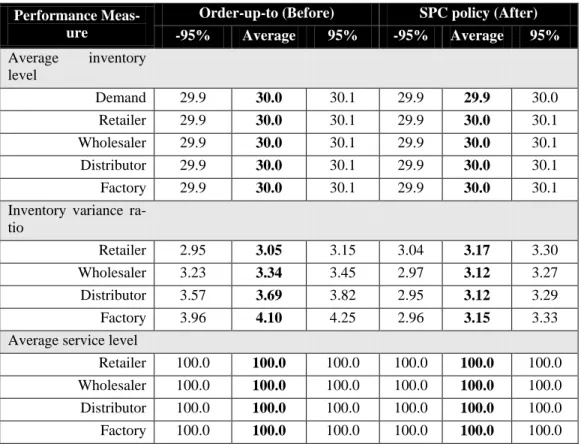
B. Inventory Behavior

The inventory behavior is a big issue for the local decision makers in the supply chain as they want to have a high service level without keeping a large safety stock. The results in Table III show that both ordering policies are successful to stabilize at the same average inventory level while achieving the same average service level throughout the supply chain. However, the SPC has achieved a better performance in terms of the inventory variance ratio than the order-up-to especially at the upstream echelons; wholesaler, distributor, and factory. The retailer has achieved a higher inventory variance ratio under the SPC than when order-up-to is applied. This can be attributed to the high level of smoothing of orders placed by the retailer whilst receiving demand of higher variance to some extent. This situation could be altered by reducing the width of the safety zone on the demand

control chart, i.e., decreasing the value of i D

K , to make the SPC policy more sensitive to demand/incoming

or-der changes. However, this action is not important because this higher inventory variance ratio does not have a significant impact on the average service level at the retailer where the retailer was able to satisfy 100% of the customer demand immediately.

TABLE III

Inventory Behavior at All Echelons in the Supply Chain Under Order-Up-To and SPC Policies Performance

Meas-ure

Order-up-to (Before) SPC policy (After)

-95% Average 95% -95% Average 95% Average inventory level Demand 29.9 30.0 30.1 29.9 29.9 30.0 Retailer 29.9 30.0 30.1 29.9 30.0 30.1 Wholesaler 29.9 30.0 30.1 29.9 30.0 30.1 Distributor 29.9 30.0 30.1 29.9 30.0 30.1 Factory 29.9 30.0 30.1 29.9 30.0 30.1

Inventory variance

ra-tio

Retailer 2.95 3.05 3.15 3.04 3.17 3.30

Wholesaler 3.23 3.34 3.45 2.97 3.12 3.27

Distributor 3.57 3.69 3.82 2.95 3.12 3.29

Factory 3.96 4.10 4.25 2.96 3.15 3.33

Average service level

Retailer 100.0 100.0 100.0 100.0 100.0 100.0

Wholesaler 100.0 100.0 100.0 100.0 100.0 100.0

Distributor 100.0 100.0 100.0 100.0 100.0 100.0

Factory 100.0 100.0 100.0 100.0 100.0 100.0

An order-up-to policy is optimal in the sense that it minimizes the inventory cost (i.e., expected holding and shortage costs). However, some authors have been worried about the trade-off between bullwhip effect and in-ventory variance [28] where a replenishment rule might smooth the orders variability but this would be on the expense of inventory variation and service level. Here, we introduced a new, simple, ordering policy that can account for both orders and inventory variability. This could be a good choice by supply chain managers to con-trol their ordering and inventory systems.

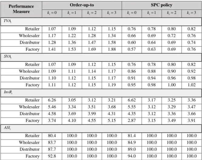
V. SENSITIVITY ANALYSIS

With using the above simulation settings, we have further investigated the sensitivity of the supply chain

per-formances to the safety stock level (k_i) under both ordering policies. The sensitivity analysis results are

summa-rized in Table IV. It can be observed that the TVAiand InvRi values are increasing as the safety stock level

in-creases whatever the applied ordering policy. However, the increasing rate is much higher when the order-up-to is applied. This confirms the findings in the literature for the order-up-to policy [14]. Also, the SPC policy was stable even when the safety stock level was low as we can see that the SPC outperforms the order-up-to in terms

of average service level when there is no safety stock (i.e., ki =0).

It can be concluded that the SPC will be able to eliminate the bullwhip effect at high levels of safety stock whilst keeping a competitive inventory performance at all echelons. However, it is still needed to do further analysis on the impact of the variation of the different parameters of the SPC policy on the supply chain dynam-ics. It is also worth investigating the performance of the proposed SPC policy with other traditional ordering policies that allow order smoothing as in [12] and [18]. This is planned for future work.

TABLE IV

The Impact of Safety Stock Variation on Both Ordering Policies Performance Measure Order-up-to SPC policy 0 i k = ki=1 ki=2 ki=3 ki=0 ki=1 ki=2 ki=3 i TVA Retailer 1.07 1.09 1.12 1.15 0.76 0.78 0.80 0.82 Wholesaler 1.17 1.22 1.28 1.34 0.66 0.69 0.72 0.76 Distributor 1.28 1.36 1.47 1.58 0.60 0.64 0.69 0.74 Factory 1.41 1.53 1.69 1.88 0.57 0.63 0.69 0.76 i SVA Retailer 1.07 1.09 1.12 1.15 0.76 0.78 0.80 0.82 Wholesaler 1.09 1.11 1.14 1.17 0.86 0.88 0.90 0.92 Distributor 1.10 1.12 1.15 1.17 0.91 0.94 0.96 0.98 Factory 1.11 1.12 1.15 1.19 0.95 0.98 1.00 1.02 i InvR Retailer 6.26 3.05 3.12 3.21 6.62 3.17 3.25 3.36 Wholesaler 5.46 3.34 3.51 3.68 5.55 3.12 3.29 3.47 Distributor 4.58 3.69 3.99 4.31 4.35 3.12 3.36 3.66 Factory 3.74 4.10 4.55 5.15 2.87 3.15 3.49 3.91 i ASl Retailer 80.4 100.0 100.0 100.0 81.4 100.0 100.0 100.0 Wholesaler 83.7 100.0 100.0 100.0 84.9 100.0 100.0 100.0 Distributor 87.7 100.0 100.0 100.0 89.0 100.0 100.0 100.0 Factory 92.8 100.0 100.0 100.0 94.0 100.0 100.0 100.0 VI. CONCLUSIONS

Inventory control policies have been recognized as a contributory factor to supply chain dynamics problems such as bullwhip effect and inventory variance amplification. A lot of research has been conducted considering the impact of different ordering policies on supply chain performances in order to provide the decision makers some insights on how to select the appropriate policy. Recently, some authors have applied the SPC control chart in the area of inventory control, however, they have not evaluated such policies in multi-echelon supply chains. In this research, we have considered a similar approach and developed an inventory control policy that relies on individual control charts to monitor and control both demand and inventory position so that balanced orders might be placed while achieving the target service level without keeping much safety stock. We adopted a simulation approach to evaluate the proposed SPC policy and to compare it with the traditional order-up-to policy in a multi-echelon supply chain. The simulation results showed that the SPC outperforms the order-up-to policy in terms of bullwhip effect, inventory variance ratio and average service level. The SPC was generally able to eliminate the bullwhip effect without hurting the inventory performance at any of the supply chain eche-lons. The astonishing performance of the SPC in terms of bullwhip and inventory variance would motivate sup-ply chain mangers to select it for the operation of their inventory systems. However, further analysis should be done to investigate the sensitivity of the SPC to other demand patterns with autocorrelation and seasonality components. Also, further analysis should be done to compare the proposed SPC policy to other ordering poli-cies that allow order smoothing.

VII. REFERENCES

[1] Lee, H. L., V. Padmanabhan, and S. Whang. 1997. “Information Distortion in a Supply Chain: The Bullwhip Effect.” Management Science 43:546–558.

[2] Fisher, M., J. Hammond, W. Obermeyer, and A. Raman. 1997. “Configuring a Supply Chain to Reduce the Cost of Demand Uncer-tainty”. Production and Operations Management 6:211–225.

[3] Zotteri, G. 2012. “An Empirical Investigation On Causes And Effects Of The Bullwhip Effect: Evidence From The Personal Care Sec-tor.” International Journal of Production Economic 143:489-498.

[4] Klug, F. 2013. “The Internal Bullwhip Effect in Car Manufacturing.” International Journal of Production Research 51:303-322. [5] Forrester, J. W. 1958. “Industrial Dynamics—a Major Breakthrough for Decision Makers.” Harvard Business Review 36:37-66. [6] Sterman, J. D., 1989. “Modeling Managerial Behavior: Misperceptions of Feedback in a Dynamic Decision Making Experiment.”

Management Science 35:321-339.

[7] Towill, D. R., L. Zhou, and S.M Disney. 2007. “Reducing the Bullwhip Effect: Looking through the Appropriate Lens.” International Journal of Production Economics 108:444-453.

[8] Costantino, F., G. Di Gravio, and M. Tronci. 2005. "Simulation model of the logistic distribution in a medical oxygen supply chain". Simulation in Wider Europe - 19th European Conference on Modelling and Simulation, ECMS 2005, 175-183.

[9] Faccio, M., A. Persona, F. Sgarbossa, and G. Zanin. 2011. "Multi-stage supply network design in case of reverse flows: A closed-loop approach". International Journal of Operational Research 12(2):157-191.

[10] Disney, S. M., and M. R. Lambrecht. 2008. “On Replenishment Rules, Forecasting, and the Bullwhip Effect in Supply Chains. Foun-dation and Trends in Technology”. Information and Operations Management 2:1-80.

[11] Burbidge, J. L. 1984. “Automated Production Control with a Simulation Capability.” Proceedings of IFIP Conference, WG 5-7, Co-penhagen.

[12] Disney, S. M., I. Farasyn, M. Lambrecht, D. R. Towill, and W. V. de Velde. 2006. “Taming the Bullwhip Effect Whilst Watching Cus-tomer Service in A single Supply Chain Echelon”. European Journal of Operational Research 173:151-172.

[13] Chandra, C., and J. Grabis. 2005. “Application of Multi-Steps Forecasting for Restraining the Bullwhip Effect and Improving Inven-tory Performance Under Autoregressive Demand.” European Journal of Operational Research 166:337-350.

[14] Chen, F., Z. Drezner, J. K. Ryan, and D. Simchi-Levi. 2000. “Quantifying the Bullwhip Effect in A Simple Supply Chain: The Impact of Forecasting, Lead Times, and Information”. Management Science 46:436–443.

[15] Ciancimino, E., S. Cannella, M. Bruccoleri, and J.M. Framinan. 2012. “On the Bullwhip Avoidance Phase: The Synchronised Supply Chain”. European Journal of Operational Research 221:49–63.

[16] Costantino, F., G. Di Gravio, A. Shaban, and M. Tronci. 2013a. “Information Sharing Policies Based on Tokens to Improve Supply Chain Performances”. International Journal of Logistics Systems and Management 14:133-160.

[17] Costantino, F., G. Di Gravio, A. Shaban, and M. Tronci. 2013b. “Replenishment Policy Based on Information Sharing to Mitigate the Severity of Supply Chain Disruption”. International Journal of Logistics Systems and Management, forthcoming.

[18] Dejonckheere, J., S. M. Disney, M. R. Lambrecht, and D. R. Towill. 2004. “The Impact of Information Enrichment on the Bullwhip Effect in Supply Chains: A control Engineering Perspective”. European Journal of Operational Research 153:727–750.

[19] [19] D’Avino, M., M.M. Correale, and M.M. Schiraldi. 2013. "No news, good news: positive impacts of delayed information in MRP". International Journal of Management and Decision Making 12(3):312-334.

[20] Watts, C. A., C. K. Hahn, and B. K. Sohn. 1994. “Monitoring the Performance of a Reorder Point System: A control Chart Approach.” International Journal of Operations & Production Management 14:51-61.

[21] Pfohl, H. C., O. Cullmann, and W. Stölzle .1999. “Inventory Management with Statistical Process Control: Simulation and Evalua-tion.” Journal of Business Logistics 20:101–120.

[22] Cheng, J. C., and C. Y. Chou. 2008. “A Real-Time Inventory Decision System Using Western Electric Run Rules and ARMA Control Chart”. Expert Systems with Applications 35:755-761.

[23] Lee, H. T., and J. C. Wu. 2006. “A study on Inventory Replenishment Policies in a Two-Echelon Supply Chain System.” Computers & Industrial Engineering 51:257-263.

[24] Montgomery, D. C. 1996. “Introduction to Statistical Quality Control.” 3rd ed. Wiley, New York.

[25] Costantino, F., G. Di Gravio, A. Shaban, and M. Tronci. 2013c. “Exploring Bullwhip Effect and Inventory Stability in A Seasonal Supply Chain”. International Journal of Engineering Business Management, 5: 1-12.

[26] Chatfield, D. C., J. G. Kim, T. P. Harrison, and J. C. Hayya. 2004. “The Bullwhip Effect—Impact of Stochastic Lead Time, Informa-tion Quality, and InformaInforma-tion Sharing: A simulaInforma-tion study”. ProducInforma-tion and OperaInforma-tions Management 13:340-353.

[27] Disney, S. M., and D. R. Towill. 2003. “On the Bullwhip and Inventory Variance Produced by an Ordering Policy.” OMEGA: The International Journal of Management Science 31:157–167.

[28] Dejonckheere, J., S. M. Disney, M. R. Lambrecht, and D. R. Towill. 2003. “Measuring and Avoiding the Bullwhip: A Control Theo-retic Approach.” European Journal of Operational Research 147:567–590.