DeepX: A Software Accelerator for Low-Power Deep Learning Inference on Mobile Devices

DeepX

: A Software Accelerator for Low-Power

Deep Learning Inference on Mobile Devices

Nicholas D. Lane

, Sourav Bhattacharya

, Petko Georgiev

Claudio Forlivesi

, Lei Jiao

, Lorena Qendro

, and Fahim Kawsar

‡_{Bell Labs,}†_{University of Cambridge,}∗_{University of Bologna}

Abstract—Breakthroughs from the field of deep learning are radically changing how sensor data are interpreted to extract the high-level information needed by mobile apps. It is critical that the gains in inference accuracy that deep models afford become embedded in future generations of mobile apps. In this work, we present the design and implementation of DeepX, a software accelerator for deep learning execution. DeepX signif-icantly lowers the device resources (viz. memory, computation, energy) required by deep learning that currently act as a severe bottleneck to mobile adoption. The foundation of DeepX is a pair of resource control algorithms, designed for the inference stage of deep learning, that: (1) decompose monolithic deep model network architectures into unit-blocks of various types, that are then more efficiently executed by heterogeneous local device processors (e.g., GPUs, CPUs); and (2), perform principled resource scaling that adjusts the architecture of deep models to shape the overhead each unit-blocks introduces. Experiments show, DeepX can allow even large-scale deep learning models to execute efficiently on modern mobile processors and significantly outperform existing solutions, such as cloud-based offloading.

I. INTRODUCTION

Today the most accurate and robust statistical models for inferring many common user behaviors and context are built on algorithms from deep learning[1] – an innovative area of machine learning that is rapidly changing how noisy complex data from the real world is modeled. The range of inference tasks impacted by deep learning includes the recognition of: faces [2], emotions [3], objects [4] and words [5]. However surprisingly, even though such inferences are critical to many mobile apps (e.g., assistants like Siri, or mHealth apps [42]) – very few of them have adopted deep learning techniques.

Mainstream mobile usage of deep learning is primarily isolated to only to a few global-scale software companies (such as Google and Microsoft), that have the resources to build proprietary, and largely cloud powered systems (with limited mobile computation), for specific high-value scenarios like speech recognition [6]. One of the key reasons for this situation is the shear complexity and associated heavy computation, memory and energy demands of the deep learning models themselves. For example, Deep Neural Networks [7] (DNNs) and Convolutional Neural Networks [8] (CNNs) routinely use networks containing thousands of interconnected units, and total millions of parameters [2], [4]. As a result, the majority of mobile sensor-based apps, both commercially and academically, rely on classifiers with lower resource overhead (such as Decision Trees and Gaussian Mixture Models [9]);

even when they are well known to be inferior to deep learning techniques.

Existing approaches for mobile deep learning have con-siderable drawbacks. Offloading inference execution to the cloud is a natural solution, but is impractical for prolonged periods (such as, augmented reality or cognitive assistance) due wireless energy overhead. Furthermore, when network conditions are poor cloud offloading, and therefore the app itself, will be unavailable. Operating on local device CPUs are feasible for some scenarios through handcrafted small footprint DNNs [11], [12], [43]; but not only does this demand a high degree of effort and skill, it is also infeasible for the majority of existing deep learning models [2], [5], [4]. More importantly, it is these complex models where we see the transformative leaps in inference accuracy and robustness that mobile apps desperately need.

The GPUs found in most mobile devices present an attrac-tive potential solution, especially because they are well suited to the type of computation common within deep models [13]. However, GPUs can consume mobile battery reserves at an alarming rate (similar to the cost of the GPS, a notoriously power hungry sensor). As a result, GPU-only solutions (just like cloud offloading) are not suitable for apps that either frequently use inference or continuously require it for long periods.

In this paper, we take important strides towards removing the barriers preventing deep learning from being broadly adopted by mobile and wearable devices. Our central con-tribution isDeepX – a software accelerator for deep learning models run on mobile hardware. This accelerator dramatically lowers resource overhead by leveraging a mix of heteroge-neous processors (e.g., GPUs, LPUs) present, but seldom utilized for sensor processing, in mobile SoCs. Each com-putational unit provides distinct resource efficiencies when executing different inference phases of deep models. DeepX allows non-expert developers to exploit these benefits by simply specifying a deep model to run. But beyond just using various local processors, DeepX amplifies the advantages they offer through two inference-time resource control algorithms, namely: (1) Runtime Layer Compression (RLC) and (2) Deep Architecture Decomposition (DAD). Through these runtime algorithms, DeepX can automatically decompose a deep model across available processors to maximize energy-efficiency and execution time, within fluctuating mobile resource constraints such as computation and memory. When necessary, resource

overhead is scaled through the novel application of SVD-based layer compression methods to remove (primarily) any redundancy from the decomposed model blocks. Importantly, this enables low-power processors to execute even larger fractions of the deep model due to the reduction in complexity. As a result, DeepX enables otherwise impossible combinations of low-power and high-power (such as GPUs) processors to service complex deep learning models with acceptable resource consumption levels. The contributions of this research include:

∙ The first software-based deep learning accelerator that makes such models practical on mobile class hardware, without manual model-specific tuning.

∙ Two novel algorithms – namely, DAD and RLC – that offer brand new forms of resource control and optimization for deep learning on mobile platforms.

∙ A proof-of-concept prototype that validates our design. This prototype also enables a broad evaluation, including com-parisons to existing solutions using popular deep models.

II. BACKGROUND

We begin with a primer on deep learning methods, before describing their relationship to mobile apps and highlighting the opportunities that mobile SoCs offer.

Deep Neural Networks.

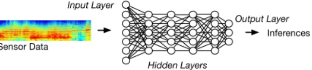
As shown in Figure 1, a series of fully-connected layers col-lectively form a DNN architecture with each layer comprised by a collection of units (or nodes). Raw data (e.g., audio, images) initialize the values of the first layer (the input layer). The output layer (the last layer) corresponds to inference classes, with units capturing individual inference categories (e.g., music or cat). Hidden layers are contained between input and output layers. Collectively, they are responsible for transforming the state of the input layer into the inference classes captured in the last layer. Every unit contains an activation function that determines how to calculate the units’s own state based on units from the immediately previous layer. The degree of influence of units between layers vary on a pairwise basis determined by a weight value. Naturally, the output of the unit also helps to determine the unit state in the next layer.

Inference (i.e., classify a sensor input) is performed with a DNN using a feed-forward algorithm that operates on each segment of data (an image or audio frame) separately. The algorithm begins at the input layer and progressively moves forward layer by layer. At each layer feed-forward updates the state of each unit one by one. This process terminates once all units in the output layer are updated. The inferred class corresponds to the output layer unit with the largest state.

Convolutional Neural Networks .An alternative formulation of deep learning are CNNs. Primarily, they are used for vision and image related tasks where are state-of-the-art [8], although their usage is expanding. A CNN is often composed of one or more convolutional layers, pooling or sub-sampling

Sensor Data

Output Layer Inferences Input Layer

Hidden Layers Fig. 1:Deep Neural Network

layers, and fully connected layers (with this final layer type being equivalent to those used in DNNs). The basic idea in CNN models is to extract simple features from the high resolution input image (2D data) and then converting them into more complex features at much coarser resolutions at the higher layers. This is achieved by first applying various convolutional filters (with small kernel width) to capture local data properties. Next follow max/min pooling layers causing extracted features to be invariant to translations, this also acts as a form of dimensionality reduction. Often before applying the pooling, sigmoidal non-linearity and biases are added.

Inference under a CNN proceeds very similarly to that of a DNN. Again, inference operates only on a single segment of data at a time. Typically sensor data is first vectorized into two dimensions (a natural representation for images). Next, these these data are provided to convolutional layers at the head of the model architecture. The net effect of convolution layers is to pre-process the data operating as a series of patches before arriving at the fully connected feed-forward layers within the CNN. Inference then proceeds exactly as previously described for DNNs until ultimately a classification is reached.

Mobile Sensing Apps. Although they come in a variety of forms and target a wide range of scenarios, the unifying element between mobile sensing apps is they all involve the collection and interpretation of sensor data. To accomplish this they embed machine learning algorithms into their app designs. DeepX is designed to be used as a black-box by developers of these mobile apps and provide a replacement inference execution environment for any deep learning model they adopt. A key dimension to this problem is the frequency at which sensor data is collected and processed; sensor apps that continuously interpret data (e.g., those targeting life-logging or mHealth) present the most challenging scenario as they may perform inference multiple times a minute; and therefore per-inference resource usage must be small if the app is to have good battery life. Apps that sense less continuously on the other hand can afford higher per inference costs. However, deep models need resource optimization before they can even execute on a mobile platform [43]; many deep models have memory requirements that are too high for a mobile SoC to support. Similarly, execution times can easily exceed limits that are accepted to an app (e.g., 30 seconds), presenting a problem even if the inference is sporadically activated by the user throughout the day. One potential solution we propose in this paper is runtime compression of fully connected deep ar-chitecture layers to reduce memory requirements and inference times (see§III-A).

in mobile devices evolve they are squeezing in an increasingly wide range of different computational units (GPUs, low-power CPU cores, multi-core CPUs). Even the Android-based LG G Watch R [16] includes a Snapdragon 400 [17] that contains a pairing of DSP and a dual-core CPU. Each processor presents its own resource profile when performing different types of computation. This creates different trade-offs for them to execute portions of a deep model architecture, depending on layer type or other characteristic. This diversity is relatively recent for mobile devices and we propose a layer-wise parti-tioning approach followed by solving an optimization equation (see §V-A) to decide how this heterogeneity should be best leveraged under various runtime conditions, e.g., instantaneous processor loads and memory availabilities. In this work, we explore this critical question facing the mobile computing community and explore within it an important aspect, namely: Can the readily available heterogeneity in mobile SoCs over-come the daunting resource barriers that currently prevent deep learning from being adopted in mobile sensing apps? In the next section, we present our answer.

III. DEEPX DESIGN

Starting in this section, and spanning the three that follow, we detail DeepX design, algorithms and prototype.

A. Design Principles

We first highlight the key issues underpinning our design. ∙ Runtime Optimization: Various methods for optimizing

deep learning models prior to execution [18], [19], [21] while useful, are insufficient. Because mobile resources (especially network connectivity) are unpredictable, even if a model has been modified to lower resource consumption, there is always the need for runtime changes. Without runtime adaption, pre-facto model changes cause resources under-utilization at times of resource scarcity, and visa versa.

∙ Do Not Ignore Low-power Processors: Matching the high computational demands of deep learning inference with high performance GPUs is a natural solution. It is also a mistake. Low-power processors (such as LPUs) can be very efficient at common inference calculations, and because of their energy efficiency can be better choices than GPUs for smaller scale DNNs. Moreover, by combining low and high energy processors, larger models can be executed still within execution time constraints, but at a reduced energy budget than high energy processors alone.

∙ Broad Deep Learning Support: The success of deep learning has resulted in thousands of model designs for many inference tasks. A natural narrow waist of com-patibility is to support both CNNs and DNNs, the two most popular deep learning algorithms today; doing so is sufficient to run thousands of existing deep models. However, other deep model varieties, such as RNNs that include sequential structure, are not currently supported.

∙ Principled Scaling of Model Resources: Adopting mobile techniques already used to manage the system resources of shallow models, such aspersonalization [22] orcontext adaption [23] is attractive. But these techniques, not built for deep learning, run the risk of damaging a deep model. Instead systems should build upon principled deep learning specific techniques (e.g., [18], [19], [21]).

B. Algorithms

DeepX aims to radically reduce mobile resource use (viz. memory, computation and energy), in addition to the execution time, of performing inference with large-scale deep learning models by exploiting a mix of network-based computation and heterogeneous local processors. Towards this goal, we propose two novel techniques:

∙ Runtime Layer Compression (RLC): A building block to optimizing mobile resource usage for deep learning is an ability to shape and control them. But existing approaches, such as those of model compression, focus on the training phase of deep learning models, rather than the inference. RLC provides runtime control of the memory and com-putation (along with energy as a side-effect) consumed during the inference phase by extending model compression principles. To provide error protection, the design seeks more conservative opportunities in redundant aspects of model representation, rather than truly simplify the model. Furthermore, by focusing on the layer level (instead of whole model), changes to a deep learning model are isolated to only where they are required. The design of RLC ad-dresses significant obstacles such as: low overhead operation suitable for runtime use, the need to retrain, and the need for local test datasets to assess the impact of model architecture changes.

∙ Deep Architecture Decomposition (DAD): A typical deep model is comprised of an architecture of many layers and thousands of units. DAD efficiently identifies unit-blocks of this architecture and creates a “decomposition plan” that allocates blocks to local and remote processors; such plans maximize resource utilization and seek to satisfy user performance goals. Existing cloud offloading algorithms can not identify the best optimization opportunities as they lack an understanding of deep learning algorithms. Distributed deep learning frameworks [13] focus on the training of algorithms and do not mix consideration for remote com-putation and local processors, that for example, operate at very distinct time-scales. DAD overcomes challenges such as a potentially prohibitive search space and inference and considering hardware heterogeneity and de- and re-composition overhead.

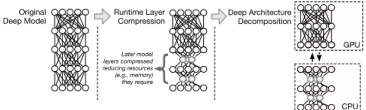
Through the combination of these two techniques, DeepX per-forms inference across a standard deep learning model with an innovative use of resources. Figure 2 provides a representative example of DeepX inference in action. A deep model that otherwise is too resource intensive for a mobile device to support in isolation, is shown to be decomposed into two

unit-Original

Deep Model Runtime Layer Compression Deep ArchitectureDecomposition

GPU CPU Later model layers compressed reducing resources (e.g., memory) they require

Fig. 2: Representative example of model decomposition and com-pression in operation under DeepX

blocks. The mobile CPU (or another constrained processor) supports initial model layers that have been compacted to meet its memory and computational limits. The remaining majority of model layers are then completed by GPU computation. Note, the model is compressed only where needed by resource constraints, instead of compression being applied across all layers. Without any compression, the CPU computation at the mobile would not have been utilized and thus wasted, for reasons as simple as a lack of local memory. Instead a better balance of layer compression and energy is reached by less compression and initial use of the CPU processor.

C. Proof-of-Concept

To demonstrate and evaluate the algorithms of RLC and DAD, and the end-to-end operation of DeepX, we develop a proof-of-concept system shown in Figure 3. We now briefly describe components of this system and how they interact within the context of a workflow.

Model Interpreter. Any already trained DNN or CNN model can be provided to DeepX. Model specifications come from developers who then incorporate the use of DeepX into the logic of a mobile or wearable app. The specification of the model describes not only the model (e.g., layer types, weight matrices, activation functions) but also information needed for inference to be performed, such as sensor type (e.g., microphone) and pre-processing steps that are applied to the data.

Performance Targets. The default semantics of DeepX are simple. It attempts to lower resources as much as possible while respecting two bounding factors. First, a single inference execution is never longer than 5 seconds, and second: the reconstruction error of any model compression (described in §IV-B) corresponds to around a 5% fall in model accuracy. Developers are free to modify these two parameters, although we expect in practice only the inference execution limit is changed. For example, an inference in response to user input may be set to 250 msec. as the user is waiting. In contrast, other inferences used for long-term tracking of activity is less time sensitive and so further resource savings can be sought. Furthermore, we expect the reconstruction error to be seldom changed as we have already set this to a very conservative value to reduce the chance any noticeable accuracy drops may occur. This behavior, and response to user inputs, is determined by a threshold described in§V-A.

Inference Interface. Requests to perform an inference using an earlier provided model are made via an API. A developer then includes an API call within a mobile app. If an app, for instance, wants to authenticate a user it can use a face recognition model like DeepFace [2]. The model reports the recognition result via the interface.

Execution Planner. Each time an inference is requested DeepX determines a new plan for execution. This enables the execution plan to be optimized for the current local device and network resource conditions. Determining this plan is the responsibility of DAD that works closely with RLC in this process. DAD examines candidate decomposition plans of the inference model and possible allocations of unit-blocks (i.e., subsections of the whole model) to all available processors. RLC allows DAD to consider an even wider set of possible execution plans by performing model compression to unit-blocks. Not only does this allow different trade-offs to be explored as the resources used by different blocks can be adjusted; but it also expands the possible matching of unit-blocks to processors, for example, by reducing the required memory of a unit-blocks to a level a processor can support. DAD also considers a variety of other factors, not only the current performance objectives; but also processor migration overhead and how certain layers are best computed by specific processor types. Of course, to arrive at a final inference result decomposed unit-blocks must have their results reassembled (see§V-B). This is also the responsibility of the Planner.

Resource Availability. Selection of a decomposition plan is strongly influenced by the current available resources. Via OS hooks DeepX receives current resource usage levels before performing an inference. But better decisions can be made using accurate predictions of resource load, and planing for predicted levels. Many approaches to resource prediction exist (e.g., [24], [25]) and could be adopted without changes to the design.

Resource Consumption. Decisions by DAD consider, of course, the resource overhead of possible decomposition plans. Doing this before execution requires estimation; this is done through the use of a coarse prediction model. Because deep learning inference is highly structured it is more predictable than arbitrary code. Even more flexible examples of mobile workloads have proven to be highly predicable [26]. DeepX also verifies predictions, and update its prediction model, by

Execution Planner Applications

Executing Deep Model

Resource Estimator

Resource Monitor

CPU GPU LPU …..

Inference Hosts Model Interpreter Inference Interface

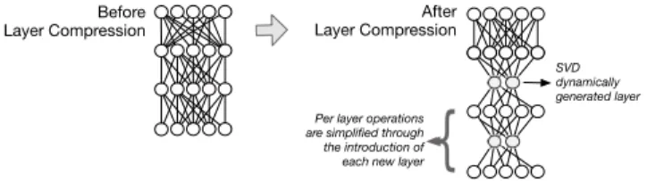
Before Layer Compression

Per layer operations are simplified through the introduction of each new layer

After Layer Compression

SVD dynamically generated layer

Fig. 4:Illustration of the RLC technique. Layer compression is shown taking place; the new generated layer is inserted into between two prior adjacent layers from the original model.

observing actual costs after a plan is selected.

Inference Host. Supporting efficient inference operations across many processor types force the use of many host implementations that include platform specific optimizations. Examples include: implementations conscious of processor ar-chitecture (decisions over fixed or floating point, awareness of cache lines) and optimized network communication (attention to the payload).

IV. RUNTIMELAYERCOMPRESSION

Through RLC, DeepX can scale the complexity of individual model layers and in doing so it controls the memory computa-tion and energy consumed by a layer during inference. DAD (see §V) strongly relies on this capability when considering possible decomposition plans for deep models; especially when plans include local processors with otherwise insufficient resources

Overview. There are two key components to RLC. First, a dimensionality reduction process (§IV-A) used to lower the computations required as one layer feeds into the next. Second, an estimator (§IV-B) that regulates the level of dimensionality reduction to be applied before model accuracy is effected beyond the intent of the DeepX user. The input to RLC is: (1) a pair of adjacent layers (𝐿 and 𝐿+ 1) from the model to be executed (as represented by weight matrices that describe their interaction); and (2), an error limit used by the estimator that describes the observed reconstruction error after dimensionality reduction is applied. Both inputs are provided by the DAD which also receives the output of RLC; specifically a replacement for weight matrix between layer 𝐿 and𝐿+1that requires fewer parameters and less computation. A. Layer Compression

Existing approaches (e.g., [18], [19], [21]) for simplifying a model require it to be re-trained as part of the process. Re-training is not practical during RLC because the Re-training of deep learning models is extremely resource intensive1 _and therefore is not feasible to perform every time the model performs an inference (in order to optimize its execution relative to available resource). We adopt the previously used method of SVD-based layer compression (such as [21]) in our design of RLC; however, our usage without training data, and for the purposes of controlling the usage of system resources is novel.

1 _{The training of deep architectures is orders of magnitude more resource}

intensive than the inference stage DeepX seeks to improve.

As a result, RLC is designed based on layer-oriented model reduction techniques specific to deep architectures that is commonly used to speed-up model training, and that impor-tantly does not require retraining. As illustrated in Figure 4, RLC adapts this approaches to control resource consumption at inference time. First the weight matrix 𝑊_𝑚𝐿+1_×𝑛 for two adjacent layers (𝐿and𝐿+ 1) with𝑚and𝑛units respectively undergoes singular value decomposition (SVD). Under SVD decomposition, the weight matrix can be represented as:

𝑊𝐿+1

𝑚×𝑛=𝑈𝑚×𝑚Σ𝑚×𝑛𝑉𝑛𝑇×𝑛 (1) Further, the weight matrix can be approximated by keeping𝑐 biggest singular values, i.e.,:

ˆ 𝑊𝐿+1 𝑚×𝑛 = 𝑈𝑚×𝑐Σ𝑐×𝑐𝑉𝑐𝑇×𝑛 (2) ˆ 𝑊𝐿+1 𝑚×𝑛 = 𝑈𝑚×𝑐𝑁𝑐𝑇×𝑛 (3)

Next, the weight matrix 𝑊_𝑚𝐿+1_×𝑛 is replaced by the product of new matrices 𝑈𝑚×𝑐 and 𝑁_𝑐𝑇_×𝑛 , which is achieved by introducing a new layer𝐿′ with𝑐≪𝑚, 𝑛units between layer 𝐿and𝐿+1. Because𝐿and𝐿+1units are fully connected, the introduction of𝐿′ causes the number of pairwise calculations and weight parameters to fall dramatically – from 𝑚𝑛 to (𝑚+𝑛)×𝑐, this in turn translates into both a lower memory requirements and lower computational load. An overview of the SVD-based compression of a deep architecture layer is given in Figure 4. Although SVD is often used by other training-time model compression approaches, our core novelty is in the use of this technique to: (1) dynamically scale resources according to availability, and (2) develop a practical version of this technique that can be applied at runtime (and not requiring, for instance, training data to be available).

Prior empirical and theoretical results support the RLC de-sign in two important ways. First, even though the architecture of the model is changed the impact on downstream layers, trained assuming the original architecture, does not typically result in large increases in error. Thus, if the product of𝑈𝑚×𝑐 and𝑁_𝑐𝑇_×𝑛 matrices accurately approximates 𝑊𝑚×𝑛, then the functional property of the original model stays similar. Second, in fact considerable amount of compression are possible, if carefully applied to certain layers, before significant accuracy declines are observed (under DeepX the degree of compression is cautiously applied by the DAD search algorithm detailed in §V-A). One reason for this is that model representations produced by training processes do not always produce the most compact representation.

B. Redundancy Estimation

Conventionally, the degree of compression to be applied is determined by running a set of off-line experiments using test data that can measure the impact on the overall accuracy. DeepX can not use this approach because analysis over test data would introduce too much overhead and require a local device to maintain large multi-GB test datasets for this purpose. RLC approaches this problem by proposing an estimator,ℰ, designed specifically to recognize redundancy in

a layer representation. The general problem of determining the relationship of model accuracy to the amount of compression applied at different layers within a model, in absence of test data, is very difficult. But by instead focusing on redundancy that corresponds to small amount of accuracy loss, the problem is made significantly easier.

The estimator ℰ computes the reconstruction error for approximating 𝑊_𝑚𝐿+1_×𝑛 with the product 𝑈_𝑚×𝑐 ⋅𝑁_𝑐𝑇_×𝑛 (see Equation 3). More specifically:

ℰ(𝑊𝐿+1

𝑚×𝑛,𝑊ˆ𝑚𝐿+1×𝑛) = √∑_𝑚

𝑖=1∣∣𝑤𝑖−𝑤ˆ𝑖∣∣22

𝑚 , (4)

where, 𝑤_𝑖 ∈ 𝑅𝑛. Additionally, as the compression can be applied to various fully-connected layers of the deep ar-chitecture, we compute the overall reconstruction error by summing all estimatedℰ across modified layers. Without the test dataset, the overall reconstruction error thus computed, provides a simple metric for measuring the deviation in model functionality. Although, overall accumulated reconstruction error (across multiple layers) follows a non-linear relationship on the effect of model performance, in our experiments we will show that small value of the reconstruction error indicates good recognition performance of the modified model.

However, users of DeepX can specify directly an upper bound as to an acceptable parameter value, or this can be done indirectly for them through loose translation of increases in error into a threshold provided to the estimator. Regulating the amount of compression applied to a layer in this way means that RLC is conservative in how much is applied. This is consistent with the design of DeepX in that the executed deep model does not deviate significantly in accuracy.

V. DEEPARCHITECTUREDECOMPOSITION

Large complex deep models are decomposed by DAD into unit-blocks that are assigned to the available local and remote processors. This allows DeepX to increase the utilization of the full range of resources available, leading to significant improvements in energy efficiency and execution latency at inference time.

Overview. DAD spans a pair of components: Decomposition Search (§V-A) and Recomposition Inference (§V-B). The first component aims to efficiently consider a range of possible decomposition plans of the deep architecture, each is assessed in terms of estimated performance (e.g., energy usage, memory requirements) relative to the provided DeepX user goals. RLC expands the search space of DAD through compression of layers within candidate plans. The second component performs inference, and arrives at a model result (e.g., classification), by recomposing the decomposed execution of model unit-blocks that are allocated to separate local- and network-based computational units. The inputs to DAD include: (1) the deep model to be executed, (2) a set of performance goals (one or more metrics from: energy, execution time, model error). The output from DAD is ultimately the inference from the provided model.

Algorithm 1 Decomposition Search

1: Input: (i) Model with 𝑛 layers, (ii) ℰ_{𝑇 𝐻} (Allowed level of overall approximation error), and (iii) 𝑒₁, 𝑒₂, . . . , 𝑒_𝑘 (Energy footprint of all available processors).

2: for all layer_𝑖∈Modeldo

3: layerType = getLayerType(layer𝑖) ⊳Identifying layer type based on operations

4: iflayerType == convolution or poolingthen 5: BlockSize = extractFilteringBlocks()

6: else ⊳Fully connected layers

7: BlockSize = extractFeedForwardBlocks()

8: for𝑗= 1to𝑃 do ⊳Extracting parameters for all processors 9: 𝐸_𝑗, 𝐵_𝑗=getProcessorParameters(BlockSize,𝑒_𝑗)

10: iflayerType == Feed-forwardthen

11: fork=90,-10,10do ⊳Linear searching parameter space 12: ℰ=CompressSVD(𝑊𝑙𝑎𝑦𝑒𝑟𝑖 𝑚×𝑛 , 𝑘)⊳Estimating Reconstruction Error 13: ifℰ<ℰ_{𝑇 𝐻}then 14: Save𝑈𝑚×𝑐and𝑁_𝑐𝑇_×𝑛 15: else

16: break ⊳Stop parameter searching

17: updateLayer(𝑙𝑎𝑦𝑒𝑟𝑖,𝑈𝑚×𝑐,𝑁_𝑐𝑇_×𝑛)

18: applyOptimization(BlockSize,{𝐸}𝑘_𝑗=1,{𝐵}𝑘_𝑗=1) ⊳using Equation 5a

19: Assignblocks to processors as identified by the optimizations

A. Decomposition Search and Optimization

Ultimately, the decomposition plan reached by DAD must reflect the currently available network- and device-based re-sources, and therefore a new plan is computed each time a model is executed. But due to the large number of units and layers that comprise typical deep models, a large variety of potential decompositions exist. Consequently, the search for this plan must balance the speed and efficiency it identifies the plan, along with the need to satisfy user performance goals.

Search. Algorithm 1 details the approach by DAD to cope with these competing concerns. Three specific techniques are employed, each narrow the search space by encoding an understanding of the deep learning algorithms and how they execute on within the resource limits presented by hardware. First, the architecture of each deep learning model includes a series of dependencies based on factors such as layer type, which determines the units must be computed in series. This limits groups of layers (Algorithm 1, line2−7) and units that can be packed together to maximize desirable properties like parallel execution. Second, hardware resource limits dictate if a unit-block of the model is viable or not (line 5 and 7). For example, a collection of units and layers may require too much memory than a particular processor can currently (or is expected to) support; in such cases the candidate partition and allocation can be ignored. Finally, levels of compression (denoted by the parameter𝑘) is estimated by allowing to retain 𝑘% variance in the weight matrix by selecting top eigen-values based on their cumulative distribution function (line 12). The resulting compression may be within the general viability for DeepX (e.g., a drop in accuracy of 5% – not considered excessive). Figure 5 illustrates an overview of the decomposition scheme described above for computational layers identified within a group.

Deep Architecture

Decomposition GPU CPU LPU

Fig. 5:Illustration of deep architecture decomposition. Different parts of the model architecture are assigned to available computational resources for runtime efficiency.

Optimization. We follow a layer wise partitioning approach and decompose the overall computations needed to evaluate the states of the nodes within a layer (e.g.,𝐿), given the states of all the nodes in the previous layer (𝐿−1), into groups of smaller computation tasks. This layer-wise decomposition strategy allows us to consistently update states of nodes within a deep architecture in a feed-forward fashion and improve overall inference efficiency. In the following, we describe the optimization approach in detail.

Unit-Block: Given a layer 𝐿, we define a unit-block as the lowest number of computations needed to update the state of a single node in that layer. Computations involved in evaluating the state of a node in layer 𝐿 is given by: 𝑥𝐿_𝑖 = 𝑔(∑_𝑗𝑥𝐿_𝑗−1⋅𝑤𝑖𝑗+𝑏𝑖

)

, where,𝑤_𝑖𝑗 is the weight connecting the 𝑖𝑡ℎ node in layer 𝐿 with the𝑗𝑡ℎ node in layer 𝐿−1, 𝑏𝑖 is the bias term and𝑔(⋅)is the non-linear function. The total number of unique blocks in a layer is the number of nodes𝑁 present in the layer. The decomposition task can be viewed as identifying a suitable number of blocks and then assigning them to an available resource.

Allocation: Formally, let 𝒫 = {1,2, ..., 𝑃} be the set of processors available in the system,𝐵𝑖,∀𝑖∈ 𝒫be the number of blocks assigned to processor 𝑖, and 𝐿𝑖 be the load limit of processor 𝑖. Further, let 𝐸_𝑖 and 𝑇_𝑖 denote the energy and the time needed to compute a single block on processor 𝑖 respectively. The optimization problem, which minimizes the overall energy consumption and execution time, can be formulated as follows: min. 𝛼 𝑃 ∑ 𝑖=1 𝐸𝑖𝐵𝑖+𝛽max 𝑖∈𝒫{𝑇𝑖𝐵𝑖} (5a) s.t. 𝑃 ∑ 𝑖=1 𝐵𝑖=𝑁 𝐵𝑖≤𝐿𝑖,∀𝑖∈ 𝒫, 𝐵𝑖≥0, 𝐵𝑖∈ 𝒵,∀𝑖∈ 𝒫,

where 𝒵 is the set of integers. Note that 𝛼, 𝛽 ≥ 0 are the weights that can be tuned to achieve any arbitrary trade-off between energy and time. The inputs𝑃,𝐸_𝑖and𝑇_𝑖are platform specific, and we estimate them by running a large number of experiments and taking the average.

We can transform (5a) to a Mixed Integer Linear Program (MILP) by introducing an auxiliary variable 𝐴, replacing max𝑖∈𝒫{𝑇𝑖𝐵𝑖} by 𝐴, and adding the constraint 𝑇𝑖𝐵𝑖 ≤ 𝐴,

Krait CPU — Core 1 Hexagon DSP

Krait CPU — Core 2

Krait CPU — Core 3

Krait CPU — Core 4

Adreno GPU Connectivity 4G LTE, WiFi BT, FM, USB (a)Snapdragon 800 DDR3 DDR3 DDR3 DDR3 Memory Controller L2 L2 Cache ARM ARM ARM ARM 192-core CUDA GPU Low Power Core (ARM CPU)

(b)Tegra K1

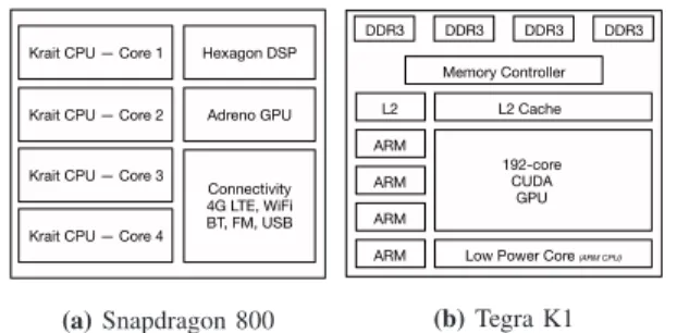
Fig. 6:Internal Architecture of SoCs used for DeepX Prototype

(a)Snapdragon 800 (b)Tegra K1

Fig. 7:Developer Boards for SoCs used for DeepX Prototype

∀𝑖∈ 𝒫 to the formulation, and solve the problem by invoking any standard MILP solvers, such as CPLEX [27].

B. Recomposition Inference

Although, distributed forms of model training are common, it is unconventional to attempt to decompose the execution of inference across local and remote resources. a number of im-plementation level optimizations are done after the deposition plan is determined, the necessary model parameters and model state are copied. For those components that can operate in parallel are executed in parallel, e.g., convolution tasks. Others wait until earlier dependencies are completed. To further save energy, DeepX powers down the state of the processors, if possible.

VI. IMPLEMENTATION

We conclude our description of DeepX by detailing its imple-mentation, and highlighting two prototype systems.

A. Prototype Platforms

The software described in §VI-B is implemented as two prototypes, each targeting Qualcomm and Nvidia SoCs. Before describing this software, we first provide details of each SoC; while some components are written differently for each SoC processor, in all cases components remain logically equivalent.

Qualcomm Snapdragon 800 SoC. As one of the most popular mobile SoCs, the Snapdragon 800 (Figure 7a) is already present in many phones (e.g., Nexus 5, Nokia Lumia 1520 and 930). As shown in Figure 6a, this SoC contains 3 programmable processors: a Krait 4-core 2.3 GHz CPU, an Adreno 330 GPU and the 680 MHz Hexagon DSP. To program this SoC, we use Qualcomm’s Mobile Development Platform that offers low-level DSP APIs within the Hexagon SDK.

Nvidia Tegra K1 SoC. Although not as popular as the Snapdragon, the Tegra K1 (Figure 7b) provides extreme GPU

performance. The heart of this chip, as illustrated in Figure 6b, is the Kepler 192-core GPU which is coupled with a 2.3Ghz 4-core Cortex CPU and an extra low-power5𝑡ℎcore (LPC) (that is designed for energy efficiency). The K1 SoC is used in the Nexus 9, Google’s phone prototype within Project Ara [28], and even high-end cars [29]. It is also used in IoT devices like the June Oven [30]. Executing code on the LPC requires the toggling of linux system calls, while access to the GPU is available from CUDA drivers [10].

B. Prototype Components

We now detail prototype components. Our Tegra version is written in Lua and C++, in contrast the Snapdragon prototype replaces Java for Lua. Each prototype spans 7.1k and 4.8k lines-of-code, respectively.

Model Interpreter. Any CNN or DNN is supported; a model is described to the interpreter as a JSON encoding of model architecture and parameters. This input also specifies details like the input sensor, sampling rates and pre-processing steps. Model file formats of deep learning toolkits, such as Torch [31], are also accepted.

Inference APIs. Mobile apps at runtime interact with the accelerator via a simple API. The two primary API calls are for: (1) providing new input data (e.g., audio clip); and (2) collecting inferences (e.g., recognized objects). Optional call parameters set target execution time and reconstruction error (recall §IV-B).

OS Interface. Because DeepX reacts to changes in system resources (e.g., available memory, processor load), the accel-erator needs to track these closely. This provided by a thin wrapper inside DeepX that uses Android APIs (in the case of the Snapdragon port) and exposed file-system bindings (for the Tegra).

Execution Planner. As suggested by Figure 3, the Execu-tion Planner is the hub of DeepX operaExecu-tion. It is invoked when inference is required (either by API call, or due to a pre-defined sampling rate). Given current system resource conditions it manages and optimizes the execution of the specified deep model against raw data from the sensor. As a result, the implementation of this planner includes both RLC and DAD, along with estimators for per-plan resource usage. For RLC and DAD, we adopt well-known high-speed (and portable) libraries for commonly occurring operations; for example, SVD operations use SVDPACKC [20] and mixed integer linear program solving is based on CPLEX [27]. Estimators of resources required by candidate plans based on spline regressions performed with python libraries. Factors like memory or computation time are predicted based on large-grain deep model characteristics (number of layers and units, type of layers); regressions are updated as models execute and provide additional data, per processor energy profiling (an offline step) allow execution time to be mapped to energy consumption. We find techniques like [26] are relatively easily adapted for this process.

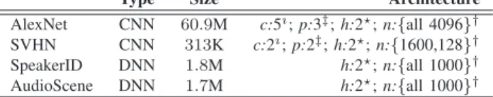
Type Size Architecture

AlexNet CNN 60.9M c:5𝚤;p:3‡;h:2★;n:{all 4096}† SVHN CNN 313K c:2𝚤;p:2‡;h:2★;n:{1600,128}† SpeakerID DNN 1.8M h:2★;n:{all 1000}† AudioScene DNN 1.7M h:2★;n:{all 1000}†

𝚤_{convolution layers;}‡_{pooling layers;}★_{hidden layers;}†_{hidden nodes}

TABLE I: Representative Deep Models

Inference Host. We implement 5 different inference hosts, 2 for the Qualcomm (viz. CPU, DSP) and 3 for the Nvida (viz. CPU, GPU, LPC). Each host is customized for the specific processor, given its limitations (such as memory) and strengths (e.g., instruction set, or architectural aspects for efficient deep layer/unit calculations). Code also carefully considers cache/memory block size when deciding how to chunk data processing operations.

VII. EVALUATION

In this section through a comprehensive set of experiments, we examine the benefits and design choices of DeepX. A. Methodology

The following setup is general to all the experiments we per-form. For those experiments that alter this setup we discuss this at the point of presenting results. Unless otherwise stated the energy and latency measurements reported are for performing a single inference. In other words, recognizing the objects in a single image, or classifying a single audio clip. Where we refer to the cloud we use average WiFi performance of 5Mbps and strong signal strength (unless otherwise stated). No resources used by the cloud are considered, but all device side data processing costs are included (such as inference computation, and network transmission); note, sensor sampling costs are not reflected in any evaluation.

Representative Workloads. We use in total four deep learning models, described in Table I. One of these is a large-scale model having over 60.9M parameters, two models are moderately large, respectively having 1.8M and 1.7M parameters. These models were originally conceived to run on the cloud. We use one CNN and two DNNs of this type. We also test a relatively small-scale CNN model with 313K parameters to test performance improvements of models under DeepX.

AlexNet. Our first large-scale model – AlexNet (CNN) per-forms object recognition [4] and supports more than 1,000 object classes (e.g., dog, car). It is the most complex model studied (60.9M parameters). In 2012, it offered state-of-the-art levels of accuracy for well-known datasets like ImageNet. SpeakerID. For our first moderately learge-scale model, we implement a 2-hidden layer (each comprising of 1000 nodes) DNN and train to identify the speakers among 106 participants (45 male and 61 female) from text-independent audio signals as provided in the Automatic Speaker Verification Spoofing and Countermeasures Challenge Dataset [39]. This speech recognition model is designed to be run continuously and has more than 1.8M nodes.

SVHN. Our first smaller scale model [32] is a CNN that is designed to read images of house numbers captured in natural settings. SVHN has been used to recognize such numbers from Google Streetview images.

AudioScene. Our second moderately large-scale model fol-lows similar architecture as in the speaker identification task (2-hidden layer DNN) and we train the model to identify among19different ambient audio environments. Examples of the audio environment includes ‘busy street’, ‘plane’, ‘bus’, ‘cafe’, ‘student hall’ and ‘restaurant’. This dataset is publicly available [40] and contains over 1500 minutes of audio scenes. This audio recognition model has over 1.7M nodes.

Baselines. We report comparisons approaches that include those that are conventional (e.g., use of the CPU only and use of cloud offloading) and rare (e.g., directly using the DSP, LPU, GPU on mobile SoCs). When we report results using the cloud, GPU, LPU, DSP or CPU then these do not involve any other computational units. For some detailed results (such as Figure 8, we also report various cloud partition splits (i.e., a fraction of the computation is done locally on the CPU, with the remainder on the cloud) to indicate the possible trade-offs in execution and energy in relation to those that DeepX enables. Cloud results consider of course the networking energy and latency of transmitting either raw sensor data or intermediate model state information (in the case of inference being partitioned).

In comparison to these baselines, DeepX is free to use any supported unit, and has constrained use of RLC; specifically we only set ℰ_{𝑇 𝐻} to allow expected accuracy drops of<5%. To validate the accuracy drop, we use the original datasets used to train the respective models and run a large number of offline experiments with varying parametric settings used for RLC and DAD (See Algorithm 1). We empirically validate that this expectation is met, and in no case find a drop greater than 5%. We note however, that this threshold of 5% that we use in this paper is somewhat arbitrary and the actual range of importance will be highly application dependent. Thus it is a tunable parameter of the system, and within our evaluation we provide examples of how changing this alters resource consumption (such as in Figure 9).

B. Energy and Execution Time Benefits

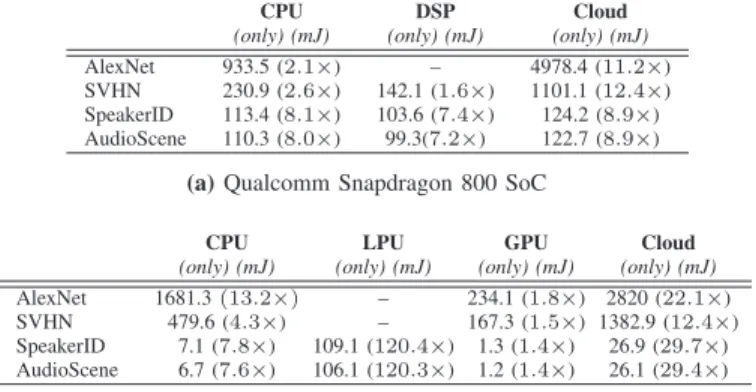
Table II summarizes the improvements to energy efficiency we observe when using DeepX to execute each deep model. Each table reports energy efficiency in terms of how many multiples of additional energy are consumed if executing each model on any of the available processor within the target SoCs (Tegra or Snapdragon). For example, when SpeakerID is running on the Snapdragon it will use a factor of 8.9× (given within parentheses) more energy if executed using the cloud than under DeepX. These tables are calculated assuming no additional background load on any processor, and with multiple execution time requirements set (viz. 100, 500 and 2000 msec.) – average values are reported. Across all model and processor combinations, the mean energy benefit

CPU DSP Cloud

(only) (mJ) (only) (mJ) (only) (mJ) AlexNet 933.5 (2.1×) – 4978.4 (11.2×) SVHN 230.9 (2.6×) 142.1 (1.6×) 1101.1 (12.4×) SpeakerID 113.4 (8.1×) 103.6 (7.4×) 124.2 (8.9×) AudioScene 110.3 (8.0×) 99.3(7.2×) 122.7 (8.9×)

(a)Qualcomm Snapdragon 800 SoC

CPU LPU GPU Cloud

(only) (mJ) (only) (mJ) (only) (mJ) (only) (mJ) AlexNet 1681.3(13.2×) – 234.1 (1.8×) 2820 (22.1×) SVHN 479.6 (4.3×) – 167.3 (1.5×) 1382.9 (12.4×) SpeakerID 7.1 (7.8×) 109.1 (120.4×) 1.3 (1.4×) 26.9 (29.7×) AudioScene 6.7 (7.6×) 106.1 (120.3×) 1.2 (1.4×) 26.1 (29.4×)

(b)Nvidia Tegra K1 SoC

TABLE II:DeepX needs only a fraction of the energy required by methods that do not decompose a model across available processors, and do not remove redundancy. Latency gains are also present, but we emphasize here benefits to energy consumption. (Average reported energy gains assuming maximum execution time set to 100, 500, and 2000 msec.)

of DeepX is 7.12×(Snapdragon) and 26.7×(Tegra) relative to each baseline. We note that in these tables some individual processors are unable to execute specific deep models (such as AlexNet on the DSP of snapdragon), we find this is either (1) due to a lack of memory on the processor along with the fact none of the baseline have the ability to the reduce model size like DeepX; or (2) they are unable to match any execution time requirement.

Figure 8 provides a more detailed view of the improved resource trade-offs that DeepX can enable, when 500 msec. execution time (only) is considered for two models: AlexNet and SpeakerID. In each case, DeepX provides the lowest energy and is always under the time requirement (500 msec). Additionally, we compare against an expanded set of baselines that include a range of cloud partitioning of the model. While running the model execution using various processors, often they are unable to meet the execution time requested, they only provide best effort. In the case of cloud offloading, a combination of cloud splits are shown, which further highlight that the energy/latency trade-offs are much poorer than DeepX. We do not show these cloud trade-offs in the prior Table II to keep the comparison clear.

Contrary to running all the computations on a specific processor, DeepX allows for alleviating high memory require-ments for deep models by partitioning of layers and then utilizing unused hardware like the DSP (without requiring any model compression). For example 93% of the total memory needed for AlexNet is concentrated only in two fully con-nected layers [44]. Model partitioning employed by DeepX allows us to overcome the need for huge memory before inference can be started. Moreover, given a relatively large execution time (e.g., 500 m sec) requirement, high energy-demanding processors, e.g., GPU, can be put to sleep sooner and one or more low power cores can be utilized to compute the residual task to minimize the overall power consumption.

(a)AlexNet – Snapdragon (b)AlexNet – Tegra (c)SpeakerID – Snapdragon

Fig. 8:Benefits to both execution time and energy consumption are observed under DeepX against a variety of baseline runtime strategies. AlexNet is shown running on both platforms and SpeakerID is shown to run on snapdragon with a requested execution time of 500 msec.

Fig. 9:Memory requirement of AlexNet under DeepX

C. Safely Identifying and Leveraging Redundancy

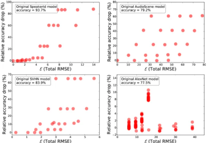
The objective of RLC is to identify redundancy within deep models to be exploited, allowing system resources to be managed but without overly impacting accuracy. Table III shows a key result. Our experimental setup seeks to constrain accuracy loss to 5% or less (compared to the original model before any changes are made). Here we show the result of RLC being applied to each deep model we test. We find that a large amount of model parameter reduction is possible, on average > 75%, while no model suffers a drop in accuracy of more than 4.9% (AlexNet). Importantly, RLC uses an estimator threshold (ℰ, see §IV-B) for each model to limit the accuracy drop. Here, e.g., we set ℰ to be 12 (RMSE) for AlexNet, a value we find through empirical testing. However, to understand the relationship between overall reconstruction error and accuracy drop, in Figure 10 we summarize extensive experimental results from all the four deep models for various compression amounts. Interestingly, for all the models the relationship between RMSE and accuracy drop is highly non-linear. However, smaller RMSE values indicate smaller accuracy drops for all the models. DeepX exploits this fact while searching for better resource utilization (see Algorithm 1). Figure 10 also exhibits instances, where a high RMSE also results in a small accuracy drop. Clearly, further theoret-ical research is required to fully understand the relationship between RMSE and accuracy drop. The current heuristic, i.e., minimizing RMSE with an empirically determined threshold, allows developers to operate without requiring time consuming re-training for models evaluated so far.

Figure 9 provides a detailed view for a single model (AlexNet) of the same overall results presented in Table III. We report results here for a single model running on the Tegra hardware, but the trends we describe are seen in all other deep models. Here we use RLC to examine how much redundancy is identified when executing DeepX under varying operating conditions, such as requests to execute the model with faster or slower execution times or processor loads. De-pending on these conditions RLC, in combination with DAD, attempts to remove different amounts of redundancy. Figure 9 shows AlexNet can be compressed significantly allowing large amounts of resources to be saved when necessary. Note, these savings are discovered by DeepX on demand; in theory a developer could apply ideas from RLC to find similar savings for a specific set of resources. But a core idea of DeepX, is for this to be doneat runtime, and change a model requested to be executed as little as possible while operating within the resources available and the performance targets expressed.

Figure 10 also shows the impact of ℰ. A cluster of redun-dancy results are shown that cause an accuracy loss greater than 5%. However, these are only identified by RLC when the estimator threshold is changed, and a few iterations performed. All other results shown, that are consistently below the target threshold, occur with the ℰ threshold set. This is another of the core innovations of DeepX. Here we show it is possible to limit the accuracy drop, and reduce the size of the model significantly without datasets that are impractical to reside on mobiles simply for performance tuning.

Existing approaches first apply an offline compression of deep models using SVD, and then use the compressed model for all inference tasks. This approach, however, does not allow application developers to control the accuracy and energy trade-offs. Depending on the application scenarios, developers can accommodate a small drop in recognition accuracy (e.g., 5%), when the resource gain is significant. Not only memory benefits, smaller models also improve the overall execution time and help to improve overall battery life. DeepX allows accuracy and energy trade-offs by applying dynamic model compressions using RLC under various user defined accuracy requirements. The opportunity of resource trade-offs under DeepX is also highlighted in Figure 9, which shows that the requirement on recognition accuracy significantly influences the memory foot print of the model. For example, in case of the

Relative Accuracy Memory Loss (%) Reduction (%) AlexNet 4.9(77.5 to 72.6) 75.5(233 MB to 57 MB) SVHN 0.2(83.9 to 83.7) 58.8(16 MB to 7 MB) SpeakerID 3.2(93.7 to 90.5) 92.8(28 MB to 2 MB) AudioScene 4.3(79.2 to 74.9) 77.8(27 MB to 6 MB) TABLE III: Model size reduction relative to accuracy loss, when applying the estimator threshold. Large reductions are clearly possible with only a small impact on accuracy. Note, for all deep models the accuracy does not drop more than the targeted 5% due to the use of the redundancy estimator.

Fig. 10:Loss in accuracy under RLC for varying estimator threshold values for the four models. By altering the threshold, the impact on accuracy can be limited as needed.

SpeakerID model, an allowance of 5% drop in accuracy runs 5.8 times faster (0.54 ms on Tegra) than the model allowing only 1% drop (3.16 ms on Tegra). Thus DeepX can adjust the model size dynamically based on the memory availability and can be deployed to new hardware platforms with different memory sizes without requiring system changes.

D. Decomposition and Assignment to Processors

The main objective of the decomposition and the assignment operation is to divide the computational task into smaller groups of blocks and assign them to the available processors, such that the overall energy-consumption and latency remain low. In the following we summarize the performances of executing the optimization on both tegra and snapdragon while running the AlexNet inference. The optimization equation (Equation 5a) requires platform specific parameters for its execution, which we compute by running experiments with a different block size on each processor and then fitting a linear model for generalizability. For the tegra this is done for: LPU, CPU, GPU; for snapdragon this is done for DSP, CPU.

On tegra, the average runtime for the optimization solver is around 14.1 ms per layer and 92.3 ms on snapdragon. Note that, often the optimization solver does not need to run repeatedly for each layer of the deep architecture, as often the block size and processor loads remain similar (after evaluating the state of all nodes in a layer). Thus the overall runtime of the optimizer remains much smaller than the inference time needed to evaluate the entire model architecture.

VIII. LIMITATIONS

Network Layout Optimization. Currently DeepX is appli-cable to the widespread varieties of deep learning networks, namely CNNs and DNNs, but not to others such as those cap-turing temporal information. In addition, the observed perfor-mance gains will vary depending on the network architecture since some layer types (e.g., feed-forward vs. convolution) benefit more than the others. Models that have been already optimized for embedded scenarios (typically by hand, e.g., [11]) are not expected to experience significant gains from RLC, although DAD is likely to still boost performance.

Changes in Resource Availability. DeepX performs per-inference optimization across memory, energy and latency, but we have not shown how it adapts to changes in the availability of device resources (such as network connectivity or CPU load) within the execution time frame. This is a limitation in our evaluation and we plan to address it in future work. Statically optimized models, as shown in [38], will perform poorly when the assumptions about resources do not hold.

Novelty of SVD Compression. Although the SVD approach to compressing layers in itself is not novel [21], we find novel ways of applying the compression technique at runtime for resource scaling and without the need for training data. The latter extension is shown to work well empirically, but more models and architectures need to be tested and a better theoretical study is required to understand how much we can compress before significant accuracy losses begin to emerge.

Resource Need Estimator. We use a simple model to estimate how the candidate layout configurations will use energy, memory, etc., and our initial findings suggest the model works fairly well. However, a more rigorous approach to predicting resource needs and adaptation to fluctuations is desirable.

Maximizing Hardware Usage. At the moment DeepX use the GPU and CPU resources na¨ıvely, without considering the underlying hardware architecture. Targeted optimizations that thoroughly make use of the hardware specifics would complement our approach with even higher performance gains.

Deep Learning Hardware. Although, DeepX is not tested on purpose built hardware for deep learning [41], [45], our software approach to accelerating models in general should apply in this case. However, the potential gains we see in software may complement the produced hardware gains resulting in both approaches amplifying each other’s benefits.

IX. RELATEDWORK

Some of the strongest examples of successful deep learning systems for mobile devices today come from industry. For example, Google has enabled forms of its deep machine translation models to run directly on a phone [36]; deep learning has already transformed commercial mobile speech recognition [37]. Technical details for these systems are usu-ally sketchy. But these few examples rely on manual per-model optimizations, provided by teams of people with high-levels of expertise in deep learning and mobile devices. In contrast,

DeepX aims to allow any developer to use deep learning methods and automatically lowers resource usage to levels that are feasible for mobile devices.

Similarly, researchers have also demonstrated one-off opti-mizations such as [33] that scaled down DNNs to run directly on a DSP only, offering energy efficiency. Others also propose deep models that are much smaller than normal and so can run on phones [11], [12]. DeepX instead targets full-scale deep models that otherwise only appear in cloud systems.

Hardware specialization is another promising direction for deep learning optimization with many studies already un-derway [41], [45]. However often these prototypes perform a specific type of deep learning (such as a CNN) or only certain types of deep model layer types (e.g., a convolution), with remaining layers executed as normal. Furthermore, we also expect DeepX will leverage specialist hardware as they become more available.

Use of more general-purpose low-power processors [46] have proven especially effective for continuous sensing types of applications. Systems like SpeakerSense [47] or DSP.Ear [48] apply application-level optimizations to balance the com-putational workload between the main CPU and the assisting co-processor. However, neither of these systems considers the n-way division by DeepX (viz. CPU, GPU, LPU or DSP).

X. CONCLUSION

In this paper, we have presented the design, implementation and evaluation of DeepX – a first-of-its-kind software ac-celerator that offers forms of resource optimization that are critical when using the best available learning algorithms, namely deep learning models, that are notably absent from mobile usage today. We believe our design and results will promote much needed further research into sensor processing and mobile machine learning inference. More importantly, DeepX shows that the bleeding edge of machine learning – as it currently manifests in deep learning – can actually run on the latest mobile hardware, all with a reasonable energy and latency performance.

REFERENCES [1] Y. Bengio, et al., “Deep learning,” MIT Press 2015

[2] Y. Taigman, et al., “Deepface: Closing the gap to human-level perfor-mance in face verification,”CVPR ’14

[3] Y. Kim, et al., “Deep learning for robust feature generation in audiovisual emotion recognition,”ICASSP ’13

[4] A. Krizhevsky, et al., “Imagenet classification with deep convolutional neural networks,”NIPS ’12

[5] A. Y. Hannun, et al., “Deep speech: Scaling up end-to-end speech recognition,”CoRR, vol. abs/1412.5567, 2014.

[6] G. Hinton, et al., “Deep neural networks for acoustic modeling in speech recognition,”Signal Processing Magazine, 2012.

[7] G. E. Hinton, et al., “A fast learning algorithm for deep belief nets,” Neural Comput., vol. 18, no. 7, pp. 1527–1554, Jul. 2006.

[8] Y. LeCun, et al., “Gradient-based learning applied to document recog-nition,”Proc. of IEEE, vol. 86, no. 11, pp. 2278–2324.

[9] C. M. Bishop,Pattern Recognition and Machine Learning (Information Science and Statistics). Springer-Verlag, 2006.

[10] “Nvidia CUDA,” http://developer.nvidia.com/cuda-zone

[11] G. Chen, et al., “Small-footprint keyword spotting using deep neural networks,”ICASSP’14

[12] E. Variani, et al., “Deep neural networks for small footprint text-dependent speaker verification,”ICASSP ’14

[13] J. Dean, et al., “Large scale distributed deep networks,” inNIPS ’12

[14] “Qualcomm Snapdragon 800,” https://www.qualcomm.com/products/ snapdragon/processors/800

[15] “Nvidia Tegra K1,” http://www.nvidia.com/object/tegra-k1-processor. html.

[16] “LG G Watch R,” https://www.qualcomm.com/products/snapdragon/ wearables/lg-g-watch-r.

[17] “Qualcomm Snapdragon 400,” https://www.qualcomm.com/products/ snapdragon/processors/400.

[18] Y. Gong, et al., “Compressing deep convolutional networks using vector quantization,”arXiv preprint arXiv:1412.6115, 2014.

[19] T. He, et al., “Reshaping deep neural network for fast decoding by node-pruning,”ICASSP ’14

[20] “SVDLIBC,” http://tedlab.mit.edu/∼dr/SVDLIBC.

[21] J. Xue, et al., “Restructuring of deep neural network acoustic models with singular value decomposition,”Interspeech ’13

[22] E. Miluzzo, et al., “Darwin phones: The evolution of sensing and inference on mobile phones,”MobiSys ’10

[23] H. Lu, et al., “Stresssense: Detecting stress in unconstrained acoustic environments using smartphones,”UbiComp ’12

[24] K. Czajkowski, et al., “A resource management architecture for meta-computing systems,” inJob Scheduling Strategies for Parallel Process-ing. Springer, 1998, pp. 62–82.

[25] R. Wolski, et al., “Predicting the cpu availability of time-shared unix systems on the computational grid,” inHPDC ’99

[26] C. Min, et al., “Powerforecaster: Predicting smartphone power impact of continuous sensing applications at pre-installation time,”SenSys ’15’ [27] ILOG Cplex, “12.2 User’s Manual”,IBM, 2010.

[28] “Google Project Ara,” http://www.projectara.com.

[29] “Audi self-driving car brings NVIDIA Tegra K1 front and center,” http://www.slashgear.com/ audi-self-driving-car-brings-nvidia-tegra-k1-front-and-center-25322090/.

[30] “June Oven,” http://techgage.com/news/

nvidias-tegra-k1-soc-has-made-it-into-an-oven-that-detects-what-its-cooking/. [31] “Torch,” http://torch.ch/.

[32] Y. Netzer, et al., “Reading digits in natural images with unsupervised feature learning,” NIPS workshop on deep learning and unsupervised feature learning, 2011.

[33] N. Lane, et al., “Deepear: Robust smartphone audio sensing in uncon-strained acoustic environments using deep learning,”UbiComp ’15 [34] O. Russakovsky, et al., “ImageNet Large Scale Visual Recognition

Challenge,” 2014.

[35] K. K. Rachuri, et al., “Emotionsense: A mobile phones based adaptive platform for experimental social psychology research,”Ubicomp ’10 [36] “How Google Translate squeezes deep learning onto

a phone,” http://googleresearch.blogspot.co.uk/2015/07/ how-google-translate-squeezes-deep.html.

[37] G. Hinton, et al., “Deep neural networks for acoustic modeling in speech recognition: The shared views of four research groups,” IEEE Signal Processing Mag, vol. 29, no. 6, pp. 82–97, 2012.

[38] D. Chu, et al., “Balancing Energy, Latency and Accuracy for Mobile Sensor Data Classification,”SenSys, 2011.

[39] W. Zhizheng, et al., “Automatic Speaker Verification Spoofing and Countermeasures Challenge (ASVspoof 2015) Database,”University of Edinburgh. The Centre for Speech Technology Research (CSTR), 2015. [40] A. Rakotomamonjy, et al., “Histogram of gradients of Time-Frequency representations for audio scene detection,”Technical report, HAL, 2014. [41] T. Chen, et al., “Diannao: A small-footprint high-throughput accelerator

for ubiquitous machine-learning,”ASPLOS ’14

[42] N. Lane, et al., “BeWell: Sensing Sleep, Physical Activities and Social Interactions to Promote Wellbeing,”Mobile Networks and Applications, vol. 19, no. 3, pp. 345–359, 2014.

[43] N. Lane, et al., “Can Deep Learning Revolutionize Mobile Sensing?,” HotMobile 2015.

[44] N. Lane, et al., “An Early Resource Characterization of Deep Learning on Wearables, Smartphones and Internet-of-Things Devices,” IoT-App workshop, 2015.

[45] C. Zhang, et al., “Optimizing fpga-based accelerator design for deep convolutional neural networks,”SIGDA ’15

[46] B. Priyantha, et al., “Enabling energy efficient continuous sensing on mobile phones with littlerock,” inIPSN ’10

[47] H. Lu, et al., “Speakersense: Energy efficient unobtrusive speaker identification on mobile phones,”Pervasive’11

[48] P. Georgiev, et al., “Dsp.ear: Leveraging co-processor support for continuous audio sensing on smartphones,”SenSys ’14