Bayesian sequential D-D optimal model-robust designs.

(1)

KATIlOLIEKE UNIVERSlTEIT LEUVEN

DEPARTEMENT TOEGEPASTE

ECONOMISCHE WETENSCHAPPEN

RESEARCH REPORT 0260

BAYESIAN SEQUENTIAL D-D OPTIMAL MODEL-ROBUST DESIGNS

by

A. RUGGOO M. VANDEBROEK

(2)

Bayesian sequential

v-v

optimal

model-robust designs

Arvind Ruggoo Martina Vandebroek

Department of Applied Economics, Katholieke Universiteit Leuven

Abstract

Alphabetic optimal design theory assumes that the model for which the optimal de-sign is derived is usually known. However in real-life applications, this assumption may not be credible as models are rarely known in advance. Therefore, optimal designs derived under the classical approach may be the best design but for the wrong assumed modeL In this paper, we extend Neff's (1996) Bayesian two-stage approach to design experiments for the general linear model when initial knowledge of the model is poor. A Bayesian optimality procedure that works well under model uncertainty is used in the first stage and the second stage design is then generated from an optimality procedure that incorporates the improved model knowledge from the first stage. In this way, a Bayesian V-V optimal model robust design is devel-oped. Results show that the Bayesian V-V optimal design is superior in performance to the classical one-stage V-optimal and the one-stage Bayesian V-optimal design. We also investigate through a simulation study the ratio of sample sizes for the two stages and the minimum sample size desirable in the first stage.

Keywords: sequential designs, two-stage procedure, V-V optimality, posterior prob-abilities, model-robust.

1

Introduction

Many scientific investigations study processes in which the nature of the relationship be-tween the process outcome and number of explanatory variables is unknown. In such situations, a collection of statistical techniques commonly referred to as Response Surface Methodology (RSM) has been developed (see Myers and Montgomery (1995) and Myers (1999) for more details).

(3)

More specifically, RSM is based on the premise that there exists some true physical relationship between the expectation E(y)

=

TJ of the response of interest y as a function of controllable inputs x, via physical constants 8

TJ

=

E(y)

=

h(x, 8).

The response surface h(x, 8) is typically unknown and may be in fact complex. Through a Taylor series expansion, it is assumed that within a region of interest the response surface TJ can be approximated by a linear graduating polynomial model of the form

TJ

=

E(y)

==

f'(x)f3,

where f3 is a vector of model parameters to be estimated and f is the polynomial ex-pansion of the inputs x. Under this modelling assumption a number of techniques has been developed for general exploration of the response surface, which provides invaluable knowledge in several applications in industry. The three major stages in RSM involve (1) data collection, which can be achieved by using carefully designed experiments (2) data analysis, which is related to model building and (3) optimization, having to do with searching for the best combination of input variables to optimize the response. In the sequel of this paper, we however concentrate on the data collection phase, where experi-mental design theory is involved.

An experimental design basically involves the specification of all aspects of an experi-ment. These may include the number of experimental units needed, levels of input or control variables to be used and choice of blocking factors. This is why the design of an experiment is as much an art as it is a science. The fundamental idea behind successful experimental design is that statistical inference about quantities of interest can be im-proved by appropriate choice of the input or control variables.

In all areas of experimental research work, costs and other limitations naturally dictates the parsimonious use of the available resources. Much of the statistical work on response surfaces in the literature has concerned the use of optimal design theory. The theory involves optimal selection of values of design factors under consideration within available resources.

(4)

Design optimality has gained momentum following the work by Kiefer (1958, 1959) and Kiefer and Wolfowitz (1959,1960) and has since become established in the statistical lit-erature. To apply optimal design theory in practice necessitates a criterion for comparing experiments and an algorithm for optimising the criterion over the set of experimental designs.

In the context of the classical linear model theory, the statistical model that describes the assumed relationship between the response variable denoted as y, and the m factors or independent variables Xl, ... ,Xm is usually written as

y

=

f/(X)f3

+

C, (1.1)

where f(x) is the p x 1 vector representing the polynomial expansion of x

=

[Xl, ... ,Xm ]'

and

f3

the p x

1

vector of parameters [,8l, ... ,.sp]'. Because the observations are subject to random variation, the error term c is added. The ith observation Yi can now be written as

Yi = f/(X;)f3

+

Ci, (1.2)

where Xi denotes the factor level combination for the ith observation. In experimental

design, factor level combination X; is referred to as the design point associated with the ith observation. For n observations, it is convenient to rewrite (1.1) as

y

= Xf3+

e, (1.3)

where Y

=

[YI, ...

,Yn]'

denotes the n x 1 vector of observations, X is the extended design matrix of size n x p and e = [Cl, ... ,cn]' is the n x 1 vector of random error tenns. The random error tenns are usually assumed to be independent and identically distributed with zero mean and common variance (12, i.e. E(e) = 0 and the variance-covariance ma-trix of the error terms is equal to cov(e)

=

(12In.

In the full rank model, X'X is nonsingular and (1.3) has a unique solution, namely

(1.4)

which is equivalent to the maximum likelihood estimator under normal errors.

(5)

The variance-covariance matrix of j3 is equal to

(1.5) Based on the parameter estimates (1.4), the predicted response at x is given by

y(x)

=

f/(X)j3 (1.6)

and a measure of the precision of the predicted value y(x), usually referred to as the prediction variance is

var {y(x)}

=

a2 f/(X) (X/X)-lf(x). (1.7)

Classical design optimality theory involves selecting the rows of X so as to optimize some function of the Fisher's information matrix, (X'X).

With the advent of computer-generated designs in the 1980's, various algorithms have been written to make these optimal designs available for practitioners. However these computer generated designs have also suffered serious setbacks with the criticism that the criteria they use are heavily model dependent. One of the major arguments against the use of optimal design theory is the need to specify a model for the response function, coupled with the fact that optimal designs are frequently quite sensitive to the form of the model (See for example Box (1982) or the historical review by Myers, Khuri and Carter (1989)). Usually the knowledge of the form of f in (1.1) is a weak one, since there may be little regressor knowledge before conducting the experiment. This makes it difficult to use optimality criteria in practice for RSM, as overspecification of f may result in a design with some observations wasted trying to estimate unimportant parameter effect or in the opposite scenario, underspecification of f may result in an inadequate model with not all necessary parameters being estimated.

It is thus fundamental that designs which are less dependent on the effect of model mis-specification be developed. Box and Draper (1959) were the first authors to consider this issue in depth. They argued that a more appropriate criterion for such model-robust designs is one which uses the average mean squared error over the region of interest. We include some non-exhaustive literature on the topic for the interested reader: Lauter (1974) proposed using an average criterion that measures the precision of parameter esti-mation and also deals with effective discrimination for polynomial models. Huber (1975)

(6)

has investigated the effect of model misspecification by conducting a minimax analysis. He found that optimal designs based on first-degree polynomials may be subject to con-siderable bias from quadratic terms. Cook and Nachtsheim (1982) and Dette and Studden (1995) provided some analytical solutions to Lauter designs and expanded her work to include other robust criteria. Steinberg and Hunter (1984) give a nice overview with ex-tensive references on these model-robust and model-sensitive designs.

The Bayesian approach to design optimality has gained popularity among research workers over the recent years as a way to address this problem of strong model dependence of optimality criteria. Covey-Crump and Silvey (1970) introduced the notion of Bayesian V-optimality in the linear model case. O'Hagan (1978) postulated a Bayesian model in which the dependence of

f3

on x is characterised by a prior probability distribution that reflects beliefs about the likely smoothness and stability of the true response function. The work of Chaloner (1984) who derived Bayesian design optimality criteria for estimation and prediction for the linear model has led to progress within the Bayesian optimality paradigm over the years. An extensive bibliography of Bayesian designs is present in her work. Another excellent review is found in Chaloner and Verdinelli (1995) that explain the basis of Bayesian optimality with several practical applications. The basic idea to Bayesian design optimality is to choose the design that maximizes posterior information about some or all of the f3's conditional on the prior information available.

2

Overview of design optimality

In what follows, we shall first give an overview of non-Bayesian and Bayesian design optimality for the linear model and briefly review approaches for obtaining optimal designs when initial model knowledge is poor.

2.1 Non-Bayesian optimal design theory

Design optimality was introduced as early as 1918, by Smith. However, major con-tributions to the area are attributed to Kiefer (1958, 1959) and Kiefer and Wolfowitz (1959,1960) who greatly extended previous work and introduced the alphabetic nomen-clature for optimum design. Two approaches to optimal design theory are found in the

(7)

literature. The first approach ignores the integrality constraint of the number of observa-tions at each design point. The resulting designs are called continuous or approximate. In the second approach, designs are constructed for a specified number of observations n. These designs are referred to as discrete or exact designs. In the sequel of this paper, we shall consider exact designs, since they are of practical relevance. However, knowledge of continuous designs is vital in offering insights into the construction of good practical designs for finite n.

Another important result in optimal design theory is the general equivalence theorem of Kiefer and Wolfowitz (1960) in which a design is represented by a probability measure on the predictor variable space (See Atkinson and Donev (1992) for further details).

Both (1.4) and (1.7) depend on the experimental design only through the p x p matrix

(X'X)-l and consequently a good experimental design will be one for which this matrix is 'small'in some sense. Various real-valued functions have been suggested as a measure of the 'smallness' of (X'X)-l. The most popular measure of design criterion is the V-optimality criterion which minimizes the determinant of the variance-covariance matrix of the parameter estimates. The corresponding value of the V-optimality criterion is

(2.1) Under the assumption of independent normal errors with constant variance, the determi-nant of (X'X)-l is inversely proportional to the square of the volume of the confidence region on the regression coefficients. The volume of the confidence region is relevant as it reflects how well the set of coefficients are estimated. A small

I

(X'X)

I

and hence large

I

(X'X) -11 implies poor estimation of

f3.

The A-optimal design deals with the individual variances of the regression coefficients as opposed to the V-optimal criterion which utilises both the variances and covariances of the information matrix. Since the variances of the regression coefficients appear on the diagonals of (X'X)-l, the A-optimal criteria minimizes the trace of (X'X)-l. The corresponding A-criterion value equals

(8)

The Q-optimality criterion minimizes the maximum of the prediction variance over the design region X. The Q-criterion value is given by

max var {y(x)} = max f'(x)(X'X)-lf(x). (2.2)

The V-optimal design minimizes the average prediction variance over the design region

X. This criterion is sometimes referred to as the Q criterion also. The V-criterion value is given by

V

=

ix

f'(x)(X'X)-lf(x) dx.

Excellent reviews of these alphabetic optimality criteria described above and the many others are given in Ash and Hedayat (1978), Atkinson (1982), Myers, Khuri and Carter (1989) and Atkinson and Donev (1992).

2.2 Bayesian optimal design theory

As with many other areas in statistics, Bayesian designs have experienced rapid growth over the years. The Bayesian approach provides a framework where prior information and uncertainties regarding unknown quantities can be incorporated in the choice of a design.

Lindley (1972) presented a two-part decision theoretic approach to experimental design, which provides a unifying theory for most work in Bayesian experimental design today. Lindley's approach involves specification of a suitable utility function reflecting the pur-pose and costs of the experiment; the best design is selected to maximize expected utility (Clyde, 2001).

For the linear model (1.3), the analogue of the widely known non-Bayesian optimality criteria discussed in Section 2.1, such as the V and A-optimality and others can be given a decision-theoretic justification following Lindley'S argument. For example, a utility function based on the Shannon information (1948) leads to Bayesian V-optimality (See Bernando, 1979 for details). In the case of a quadratic loss function, a Bayesian general-ization of the A-optimality design criterion is obtained. For more details on the various classes of Bayesian optimal designs and related discussions, we refer to Chaloner (1984), Verdinelli (1992), Chaloner and Verdinelli (1995), Verdinelli (2000) and Clyde (2001).

(9)

2.3

Model robust Bayesian designs

We now briefly look at designs within the Bayesian paradigm which are robust in some sense to model uncertainty. Dette (1993) developed Bayesian 'V-optimal and model robust designs in linear regression models. The interesting work by DuMouchel and Jones (1994) illustrates a very elegant use of Bayesian methods to obtain designs which are more resis-tant to the biases caused by an incorrect model. They assume that there are two kinds of model terms, namely primary and potential terms which are high and low priority terms in the model respectively. By conceiving a prior distribution on the model coefficients that takes these primary and potential terms under consideration, they generate a Bayesian 'V-optimal design by maximising the posterior information matrix. Similar type of work has been done by Andere-Rendon, Montgomery and Rollier (1997) for mixture models where they show that the performance of their Bayesian designs are superior to standard 'V-optimal designs by producing smaller bias errors and improved coverage over the factor space.

Another strategy to develop robust designs found in the literature is the use of Bayesian sequential procedures. With this approach, it is possible to develop designs in two or more stages that leads to less dependence on model specification. The idea behind the sequential designs is intuitively appealing in the sense that the experimenter could have the opportunity to revise the design and model in the course of the experiment. Box and Lucas (1959) were the first authors to introduce the idea of sequential designs. Box, Hunter and Hunter (1978) also recommend the sequential assembly of smaller experiments over designing large comprehensive experiments, whenever this is feasible.

Throughout the optimal design literature, the sequential approach has been studied and developed within the non-linear framework. This is natural as the classical alphabetic optimality criterion requires prior knowledge of the model parameters, {3 due to the non-linearity of the problem. In this context, several two-stage designs have been developed in the literature. Abdelbasit and Plackett (1983) suggested a two-stage procedure to derive optimal designs for binary responses. Minkin (1987) generalises the idea of Abdelbasit and Plackett and proposes an improvement to their two-stage proposal. Myers, Myers, Carter and White (1996) proposed a two-stage procedure for the logistic regression that uses 'V-optimality in the first stage followed by Q-optimality in the second. Letsinger

(10)

(1995) also developed two-stage designs for the logistic regression model. Sitter and Wu (1995) developed two-stage designs for quantal response studies where they may be in-sufficient knowledge on a new therapeutic treatment or compound for the dose levels to be chosen properly.

Development of two-stage designs for linear models has been limited in the literature. Neff (1996) developed Bayesian two-stage designs under model uncertainty for mean estimation models. Montepiedra and Yeh (1998) developed a two-stage strategy for the construction of V-optimal approximate designs for linear models. Lin, Myers and Ye (2000) developed Bayesian two-stage v-V optimal designs for mixture models.

3 Bayesian two-stage designs under model uncertainty

We now look in detail at the approach of Neff (1996) for developing Bayesian two-stage

V-V optimal designs in the context of linear models. For the linear model y = f/(X),l3

+E:,

a Bayesian two-stage design approach makes it possible to efficiently design experiments when initial knowledge of f is poor. This is accomplished by using Bayesian V-optimality in the first stage following the approach of DuMouchel and Jones (1994) and then the second stage V-optimal design is generated from the first stage by incorporating improved model knowledge from the first stage design.

3.1 Selection of the first stage design

Suppose that in a linear regression model such as (1.3), the regressors believed to be important in modeling the response are called primary terms and the uncertain regressors in the model are referred to as potential terms. The linear model (1.3) can thus be written as

y = Xpri ,l3pri

+

Xpot {3pot

+

e, (3.1)

where y is a vector of (n x 1) responses distributed as N(X{3, 0'21), X = (XpriIXpot) is a matrix of (n x (p

+

q)), ,l3pr; is a p x 1 vector and ,l3pot is a q x 1 vector attached to the primary and potential terms respectively. A first stage V-optimal design can be obtained along the lines described by DuMouchel and Jones (1994). We describe their procedure,

(11)

but first look at a scaling convention and some distributional assumptions they propose.

A preliminary scaling and centering is recommended by DuMouchel and Jones to minimize the correlation between primary and potential terms and to permit the use of a standard prior distribution on the coefficients. The idea of the scaling convention is to make each potential term and all primary terms orthogonal to each other over the set of candidate points. This is achieved as follows in practice: Let X

=

(XpriIXpot) represent the set of candidate points in model space. Regressing the potential terms on the primary terms results in a

=

(X;"'iXpri)-l X~riXpot' the alias matrix measuring how confounded Xpot is with X pri . Replacing Xpot by Z

=

R/(max{R} - min{R}) where R = X pot - aXpri,

essentially eliminates the aliasing over the candidates and this makes the choice of prior distributions easier.

Since the primary terms are likely to be active and no particular directions of their ef-fects are assumed, the coefficients of the primary terms are specified to have a diffuse prior distribution - that is an arbitrary prior mean and prior variance tending to infinity. On the other hand, potential terms are unlikely to have huge effects, and it is proper to assume that they have a prior distribution with mean

°

and a finite variance. The assumption N(O,72(T2I) is appropriate. The parameter 72 will determine the choice of designs, since it reflects the degree of uncertainty associated with potential terms relative to (T2. The larger the value of 7 2 , the stronger the belief in the potential terms. Under

the assumption that primary and potential terms are uncorrelated (following the scaling convention), the joint prior distribution assigned to (3pri and (3pot is N(O, (T27 2K-1) where

K is a (p

+

q) x (p

+

q) diagonal matrix, whose first p diagonal elements are equal to 0 and the remaining q diagonal elements are equal to 1.

Given the above prior distribution, the posterior distribution for the model parameters is also normal (see Pilz (1991)) and

p((3ly, (T2)

~

N [ (XIX

+

~)

-lX/y , (T2 (XIX

+

~)

-1].

(3.2)

DuMouchel and Jones's Bayesian analogue to the classical V-optimal design in the case that prior information is available is the design that numerically maximizes the determi-nant of (X'X

+

K/72 ) with respect to X. The resulting Bayesian V-optimal design will

(12)

be one which will support estimation of both {3pri and {3pot but given the structure of the K matrix, higher priority will be given to the primary terms. It can also easily be seen that as T approaches 00, the Bayesian V-optimal design becomes equivalent to the

classical V-optimal design with all (p

+

q) terms treated equally. In the case T

=

0, we end up with the V-optimal design for the primary terms model only.

3.2

Analysis of first stage design

Let us consider the usual linear model Y

=

X{3

+

e, where it is assumed that Yil{3 rv

N(X;{3, (12 I) for each stage i (i

=

1,2) with nl and n2 observations for the first and

second stage respectively. X is the (nl

+

n2) x (p

+

q) extended design matrix for the combined stages. The first stage Bayesian V-optimal design is selected as described in Section 3.1 by minimising I(X/Xl

+

K/T2)-ll.

The parameter T is unknown in the first stage and will depend on the belief the

experi-menter has on the potential terms. The larger the value T, the more certain these terms

are present in the full model. DuMouchel and Jones (1994) use the default value of T = 1 in their calculations. In the context of the two-stage procedure, Neff (1996) recommends a value of T

=

5 in both the first and second stage for its ability to produce designs which

are robust to model misspecification. Lin, Myers and Ye (2000) recommends a value of T = 1 for mixture models.

Before observing the first stage data, the experimenter has a model with (p+q) regressors. The true relationship between the response and the input variables could be one of the following three types: (i) the model contains only the p primary terms (ii) the model contains all the p primary terms and q potential terms, i.e. the full model or (iii) the

p primary terms and a subset of the q potential terms. Note that the three possibilities always include the p primary terms as these are the terms for which the experimenter has strong beliefs and hence should be present in the model. The total number of plausible models is thus m = 2q • Consequently each candidate model Mi contains all primary terms and a subset qi (0 ::; qi ::; q) of potential terms.

The attractiveness of sequential designs becomes evident now. Once the data from the first stage has been collected, the information from the analysis can be used as prior

(13)

infor-mation to reduce model uncertainty in the next stage. Model knowledge can be updated by scoring each of the plausible candidate models using posterior probabilities indicat-ing the likelihood that a particular candidate model is actually predictindicat-ing the response adequately. These resulting scores or posterior probabilities can then be incorporated as weights to a second stage criterion.

Box and Meyer (1993) suggest a general way for calculating the posterior probabilities of different candidate models within the framework of fractionated screening experiments. Neff (1996) adapted their approach couched within the sequential Bayesian designs par-adigm. We now describe her approach and adapt it to incorporate uncertainty in T2.

The Bayesian approach to model identification is as follows (See for e.g. Box and Tiao (1968)). Let us label the set of all candidate models as Mo, Ml, ... , Mm where Mo cor-responds to the primary terms model only. Each model Mi contains the parameters

f3i

= [

f3pri ] where f3 pri contains all the p primary terms and f3 pot(i) contains a subset

(3pot(i)

qi of the q potential terms so that the sampling distribution of data Yl, given model Mi

is described by the probability density !(Yl!Mi,{3;). The prior probability of model Mi

is p(Mi), and the prior density of {3i is !({3i!Mi). In the context of the first stage design, the predictive density of Yl given model Mi is given by the expression

(3.3) where Bi is the set of all possible values of (3i. Given the first stage data, the posterior probability of the model Mi given the data Yl is then

(3.4)

The posterior probabilities p(Mi!Yl) provide a basis for model identification and tenta-tively plausible models are identified by their large posterior probabilities. Now, each candidate model Mi contains the p primary terms and qi potential terms (0 ::; qi ::; q).

(14)

model. Assuming that anyone of the potential term being active is independent of beliefs about the other terms, the prior probability P(Mi) of model Mi is given by

(M) - qi(l )q-qi· - 1 2

p i - 7r - 7r , 2 - , , ... , q. (3.5)

The value of 7r should be chosen to represent the proportion of potential terms to be active. Since the experimenter may expect only a few of the potential terms to be really active, appropriate values of 7r would be in the range from 0 to 0.50. Box and Meyer (1993) found sensible results for 7r = 0.25. The analysis can be repeated for different val-ues of 7r, say 0.1,0.25, 0.5 but in general, the same factors will be identified as potentially active. Neff (1996) as well as Lin, Myers and Ye (2000) use 7r=1/3 in their computations.

Since we have assumed a normal linear model, the probability density of Yl given Mi is given by

!(YIIMi,,Bi) IX (J-n'exP[-(Yl - Xi,Bd(Yl - X i,Bi)/2(J2].

Integrating (3.3) along the lines shown in Box and Meyer (1992) and assuming that ,B1(J2, 72 ~ N(O, (J272K-l) following the scaling convention described previously, we get

(3.6) where Xi is the first stage design in model Mi space and

and

The resulting posterior probability for model Mi becomes

(3.7)

(15)

where C is the normalisation constant that forces all probabilities to sum to one.

In practice to avoid floating-point overflow, one actually computes

(3.8) for each model Mi , where Mo is the model with primary terms only. Dividing by the

constant p(MO)f(Yl\Mo) does not change the final result as all the posterior probabilities are eventually scaled to unity, but this prevents getting large numbers as intermediate results (Box and Meyer, 1993).

Using (3.5) and (3.6), the expression (3.8) becomes

(3.9) Recall that in the first stage, it is assulIl:ed that all coefficients of potential terms are specified to have a N(O,7 2(1'21) prior. The value of 7 2 is unknown and a guess value based on prior beliefs of the experimenter is used. Neff (1996) uses the same value of

T = 5 in both her first and second stage designs. We propose to update the value of 7 2

to yield f2 for use in the second stage. We follow the approach of Box and Meyer (1992) for modelling and updating the uncertainty of 7 2 . Similar type of approach for mixture

models has been proposed by Lin, Myers and Ye (2000). A convenient update of f2 is obtained as the mode of the posterior density of p(72\Yl)' Setting the prior density of

p( 7 2) to be locally uniform, i.e. substituting it with a constant, results in the posterior

density p(72\Yl) to be given approximately by

m

=

I>(Mi)p(Yl\Mi,72)

i=O

(16)

Since f is the value most likely to occur in the posterior density of T2 given YI, it is a more reasonable value to be used in all calculations after the first stage. In practice to compute f, we repeat the posterior probabilities calculations for f over a fine grid of T

values and extract the value of T that maximizes (3.10).

3.3

Selection of second stage Bayesian

V-V

optimal design

In the first stage it is assUilled that the joint prior distribution of ,610'2, T2 is N(O, 0'2T2K-I) and the resulting first stage posterior distribution of ,610'2,T2 is N(bl, VI) where bl = (XiXI +K/T2)-IXiYI and VI = 0'2(XiXI +K/T2)-I. Let the second stage

prior distribution of,6 be the first stage posterior. Assume that Y2, the n2 second stage

observations are also normal, namely, Y21,6,0'2 "" N(X2,6, 0'21), where X 2 is the second stage design expanded to full model form. Then, the second stage posterior distribution of,6 is also normally distributed with mean b2 = (XiXI + X~X2 + K/f2)-IXiYI and variance V 2 = 0'2(XiXI + X~X2 + K/f2)-1. Note that T2 has been updated to f2 in the second stage.

Since,6 contains all (p + q) parameters of the full model, a Bayesian V-V optimal design for the full model is found by choosing X 2 so as to minimize 1 (XiXI +X~X2+K/f2)-II.

However, the full model is only one of the candidate models and in most cases not the most appropriate. Let us consider our subset models Mo, Ml, ... ,Mm as discussed previously, with each model Mi defined by its parameters ,6i' The posterior variance of ,6i is now

V 2(i) = 0'2(Xi(i)XI(i) + X~(i)X2(i) + Kdf2)-I,

where X1(i) and X 2(i) are the first stage and second stage design matrices respectively, expanded to model space Mi and Ki = [Opx p Opxq,

1

is the

(P+qi)

x

(P+qi)

matrix. A

Oq, xp Iq, xq,

Bayesian

v-v

optimal design for model Mi is the set of design points X 2 which minimizes Vi=IV2(i)I· Since the posterior Box and Meyer probabilities computed from first stage data as described before reflect model importance, they can be incorporated as weights to average the V criterion when the second stage is selected. This is performed by choosing the second stage design points so as to minimize 1)i for each model Mi. In practice, this is done by choosing the second stage design points X 2 E X so as to minimize

LVi

P(MiIYl)'

M,

(17)

4

The two-stage design procedure

The two-stage design procedure is best understood by contrasting it with the single stage design. A single stage design of size N implies that all the N design points are optimally selected and executed as a group. Analysis and statistical inference are then based on the resulting N observations. In contrast, a two-stage design is one in which the N

observations are obtained by a series of two experiments run sequentially of each other. The first stage experiment is optimally designed using a certain optimality criterion, then conditional on the information provided from the first stage, the second stage design is chosen to create certain optimal criteria conditions in the combined design. Statistical inferences are then made based on all N observations obtained from the two-stages, as if it was completed in a single stage (Neff, 1996).

4.1 Effect of

r

in the first stage design

Before looking at some examples of two-stage designs, we briefly examine the effect of T

on the selection of the first stage Bayesian V-optimal design. Intuitively the parameter

T2 will determine the choice of designs as it reflects the degree of uncertainty associated

with potential terms relative to 0"2. The larger the value of T2, the stronger the belief in

the potential terms.

Let us suppose that the full model under consideration by the experimenter comprises the following regressors:

with p = 4 primary terms, {1,Xl,X2,X3} and q

=

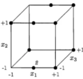
6 potential terms, {X1X2,X1X3, X2X3, X12, X22, X3 2 }. Twelve runs are allocated to the first stage. The resulting designs

for various values of T are shown in Figure 1.

It can be seen that for T

=

0.1, implying very little belief in the potential terms, the

Bayesian V-optimal design points spans at the extremes replicating four of the corner points. This is well-known with V-optimality which usually pushes design points to ex-tremes. It is not possible to estimate the quadratic effects in the potential terms. The same design points are selected for values of T up to 0.4. For T

=

0.5, the overall centroid

(18)

•

+ 1 . . - - f - - - _ .

•

X2 X2

•

+1 +1 +1 X3 X3 X3 -1 2 -1 -1 -1 -1 Xl +1 -1 Xl +1 (a) T= 0.1 (b)T=0.5 (c)T=0.6

Figure 1: First stage designs with varying TAU values

is selected. The overall center point provides some information about the quadratic terms. However, it is still not possible to obtain independent information on the potential terms. When T = 0.6, three center points, one on each of the Xl, X2, Xg planes and a mid-edge

point on the Xl plane are selected. These additional four runs enable estimation of the

potential terms. It could be seen that for T

>

0.6, the eight corner points together with

three center points and a mid-edge point on any of the planes are ever in the design. This abrupt change in the Bayesian V-optimal solution at around T

=

0.6 is also seen in the

theoretical examples presented in Section 3 of the paper by DuMouchel and Jones (1994). It can easily be seen when T

<

0.4, the Bayesian V-optimal design will be identical to the classical V-optimal for the primary terms model only. In case T 2:: 0.6, the Bayesian V-optimal design will become equivalent to the classical V-optimal design with all (p

+

q)

terms treated equally, i.e. for the full model. The classical non-Bayesian V-optimal de-signs obtained using PROC OPTEX in SAS for the primary terms and full model are shown in Figure 2 for comparison. The designs for T = 0.1 to 0.4 are identical to the primary terms model design as in Figure 2. With some rotation around the axes, the de-sign for the full model in Figure 2 is similar to the Bayesian V-optimal dede-signs for T 2:: 0.6.

We make the following concluding remark when an experiment is carried out solely in a one-stage procedure; the default value of T

=

1 proposed by DuMouchel and Jones is a good compromise to use in that context. This is also supported by the work of Lin, Myers and Ye (2000) where the default value of T = 1 works well in the first stage design for

mixture models. Neff (1996) recommends using T

=

5 in a two-stage procedure. We shall investigate further the effect of T on the combined two-stage design in Section 5.

(19)

+1 2

+1.---+--.-•

•

._---+-... +1

( a) Primary terms model (b) Full model

Figure 2: Non-Bayesian V-optimal design for the primary terms and full model

4.2

Some examples of two-stage designs

We now present a few examples of Bayesian two-stage V-'D optimal designs under different true models. Let us suppose that the full model under consideration by the experimenter comprises the following regressors:

(4.1) withp

=

4 primary terms {1,X1,X2,Xi} and q

=

4 potential terms {X3,X1X2,X1X3,X2X3}. Since the second stage design is a random variable depending on the first stage, response data from the first stage experiment are needed in the computation of the posterior proba-bilities used in the second stage criterion. We consider data simulated from three different true models under the assumption that c rv N(O, 1). A moderate value of 7r=1/3 is used

in all the examples.

CASE I

The first stage data set is simulated from the true model comprising only the primary terms {I, Xl, X2, xi} namely,

(20)

._----11-__.+1 Xg

-1 __ - ... -~-1

-1 Xl +1

Figure 3: First stage design

The coefficients of the parameters of the true model are large compared to 0"2 (assumed to be unity) thereby indicating importance of the primary terms. Ten runs are allocated to each stage of the experiment and 1" = 5 is used in the first stage. The Bayesian optimality

criterion presented in Section 3.1 is used to select the first ten runs. The resulting design is shown in Figure 3.

It can be seen that the design is desirable with all extreme points selected and two edge points on the Xl plane for estimation of {3n in the full model (4.1). Only two levels of X2 and X3 are necessary since there is no interest in estimating {322 and {333. According

to Section 3.2, the response data from the first stage are used to get the value of f. The results shown here are for one simulation data set only. Figure 4 shows the poste-rior density of 1"2 given Y1, which shows that the value of f with maximal probability

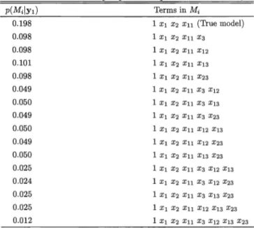
is very close to zero. This is logical considering that the true model comprises primary terms only. The first stage data and value of f is used to compute the Box and Meyer posterior probabilities associated with each candidate models according to Section 3.2. The posterior probabilities are shown in Table 1 and we clearly see that the true model 'enjoys' the highest posterior probability. Several other simulations showed similar results.

For this simulation set, ten observations of a second stage design are chosen according to Section 3.3. Figure 5 shows the second stage design. Given the true model contains only primary terms, it can be seen that in the second stage design points are selected to better estimate these terms, namely several mid-edge points on the Xl plane to estimate

{3n adequately.

(21)

0.5 1.5 2 2.5 3 3.5 4 4.5 5 5.5 TAU

Figure 4: Posterior density of 7 2 given Y1'

Table 1: Box and Meyer posterior probabilities for Mi

0.198 1 Xl X2 Xu (True model) 0.098 1 Xl X2 Xll X3 0.098 1 Xl X2 Xll X12 0.101 1 Xl X2 Xll X13 0.098 1 Xl X2 Xll X23 0.049 1 Xl X2 Xll X3 X12 0.050 1 Xl X2 Xll X3 X13 0.049 1 Xl X2 Xll X3 X23 0.050 1 Xl X2 Xll X12 X13 0.049 1 Xl X2 Xll X12 X23 0.050 1 Xl X2 Xll X13 X23 0.025 1 Xl X2 Xll X3 X12 X13 0.024 1 Xl X2 Xll X3 X12 X23 0.025 1 Xl X2 Xll X3 Xu X23 0.025 1 Xl X2 Xll X12 X13 X23 0.012 1 Xl X2 Xll X3 X12 X13 X23

(22)

+1 X2 2 +1 X3 -1 -1 -1 Xl +1

Figure 5: Second stage design

CASE II

The first stage data set is now simulated from the true model comprising all the primary terms and two potential terms {1,Xl,X2,xf,X3,XlX2} namely,

y = 50.0

+

9.2 Xl

+

11.7 X2

+

14.4

xi -

1.80 X3

+

1.3 XlX2

+

C.

The coefficients of the parameters of the potential terms X3 and XlX2 are small compared to 0"2 and thus their effect will be only marginally significant in the true model. Again ten

runs are allocated to each stage of the experiment and T

=

5 in the first stage. The first

stage design is shown as previously in Figure 3. According to Section 3.2, the response data from the first stage are used to get the value of f as previously. The results are for one simulation data set only. Figure 6 shows the posterior density of T2 given Yb which

reveals that the value of f is very close to two. This makes sense considering that the true model comprises primary terms and two potential terms whose effects are only marginally significant compared to 0"2 given the parameters assigned to them in the true model. The

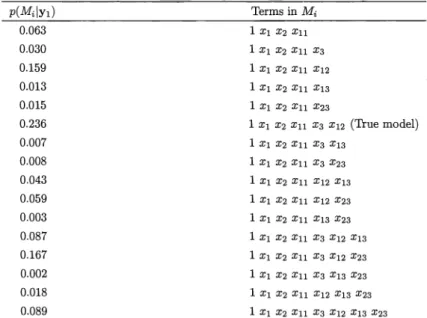
first stage data and value of f are used to compute the measure of fit associated with each candidate models according to Section 3.2. The posterior probabilities are shown in Table 2 and we clearly see that the true model 'enjoys' the highest posterior probability. Several other simulations showed similar results.

For this simulation set, ten observations of a second stage design are chosen according to Section 3.3. Figure 7 shows the second stage design. The second stage design concentrates more points in estimating the terms in the true model, replicating one of the mid-edge point on the Xl plane and selecting other mid-edge points on the Xl plane so that

(23)

18 16

O+--'~.-.--'--.--r-'.-.--.--'--o

0.5 1.5 2.5 3 3.5 4 4.5 5 5.5

TAU

Figure 6: Posterior density of T2 given Yl'

p(MiIYl) Terms in Mi 0.063 1 Xl X2 Xu 0.030 1 Xl X2 Xu X3 0.159 1 Xl X2 Xu X12 0.013 1 Xl X2 Xu X13 0.015 1 Xl X2 Xu X23 0.236 1 Xl X2 Xu X3 X12 (True model) 0.007 1 Xl X2 Xu X3 X13 0.008 1 Xl X2 Xu X3 X23 0.043 1 Xl X2 Xu X12 X13 0.059 1 Xl X2 Xu X12 X23 0.003 1 Xl X2 Xu X13 X23 0.087 1 Xl X2 Xu X3 X12 X13 0.167 1 Xl X2 Xu X3 X12 X23 0.002 1 Xl X2 Xu X3 X13 X23 0.Q18 1 Xl X2 Xu X12 X13 X23 0.089 1 Xl X2 Xu X3 X12 X13 X23

(24)

+l.._-j-e--_. X2 +1 2 x3 -1 -1 -1 Xl +1

mation of (311 is very adequate as it has major importance with its large coefficient in the true model.

CASE III

The first stage data set is now simulated from the true model comprising the primary terms and the two potential terms as in Case II {I, Xl, X2,

xi,

X3, XIX2} namely,

y

=

50.0

+

9.2 Xl

+

11.7 X2

+

14.4

xi -

6.2 X3

+

9.8 XIX2

+

c.

However, the coefficients of the parameters of the potential terms X3 and XIX2 are now

larger and thus their effect will be more significant in the true model as opposed to Case II where their effect were less prominent. Again ten runs are allocated to each stage of the experiment and 7

=

5 in the first stage. The response data from the first stage are

used to get the value of f associated with each candidate model and the results shown are for one simulation data set. The posterior density of 7 2 given Yl (Figure 8) shows that

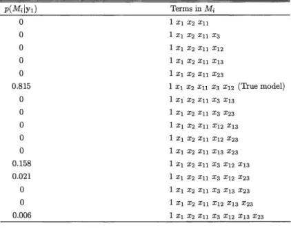
the value of f is very close to twenty-two. This is natural considering that the true model comprises primary terms and two potential terms. However, the effects of the potential terms are now much more important compared to Case II. This obviously reflects very strong beliefs in these terms and consequently leads to the large value of f to be used in the second stage design. The Box and Meyer posterior probabilities associated with each candidate model are shown in Table 3 and we clearly see that the true model has the highest posterior probability.

The ten observations of the second stage design are shown in Figure 9. Since the potential

(25)

10000000

..

8000000 0 'CIII 'sGl 6000000 III:;:; 0= a.ji 'tllll GlJl 4000000 'iijo ~a c: ::J _2000000 0 0 5 10 15 20 25 30 35 TAU

Figure 8: Posterior density of T2 given YI.

0 1 Xl X2 Xll 0 1 Xl X2 Xll X3 0 1 Xl X2 Xll X12 0 1 Xl X2 Xll X13 0 1 Xl X2 Xll X23 0.815 1 Xl X2 Xll X3 X12 (True model) 0 1 Xl' X2 Xll X3 Xl3 0 1 Xl X2 Xll X3 X23 0 1 Xl X2 Xll X12 X13 0 1 Xl X2 Xll X12 X23 0 1 Xl X2 Xll X13 X23 0.158 1 Xl X2 Xll X3 X12 X13 0.021 1 Xl X2 Xll X3 X12 X23 0 1 Xl X2 Xll X3 X13 X23 0 1 Xl X2 Xll X12 X13 X23 0.006 1 Xl X2 Xll X3 X12 X13 X23

(26)

+1..--+---..

~-_>-i---"+1

-1 *---.-1 -1 Xl +1

terms are more important than in Case II above, there is no replication of the mid-edge point on the Xl plane as in Figure 7, but the design points in the second stage spans at

the extremes again so that estimation of the potential terms parameters are adequate.

4.3

Conclusions from two-stage examples

The essence of all these examples is to demonstrate that the value of T is updated

ac-cordingly in the second stage to reflect more belief in the potential terms, should they be important in the true model. In other words, f is small if the true model contains only primary terms and becomes larger as the marginal significance of the potential terms increases relative to (J2. Also we can deduce that in general, the second stage design is

very effective in selecting design points based on information from the first stage design and considering terms present in the true model. The choice of T in the combined design

will be investigated in the next section.

Additional simulations were also conducted to study the influence of 7r on the two-stage

procedure, by repeating the analyses above using 7r

=

0.1, 0.25, 0.3 and 0.5. In general,

the procedure is quite robust to different values of 7r in the sense that usually the same

design points are selected in the second stage. The nominal value of 7r

=

1/3 has served

well, but in any case experimenters should select 7r based on their prior expectations on

the proportion of potential terms in the model.

(27)

5

Evaluation of Bayesian Two-Stage

V-V

Optimal

Designs

The performance of the Bayesian two-stage V-V optimal designs presented in Sections 3.1 - 3.3 will now be evaluated relative to the classical one-stage designs. Since the second stage design is a random variable dependent on first stage data through the Box and Meyer posterior probabilities, we need a simulation approach to evaluate the performance of the two-stage procedure. We make use of the equality for the variance of a random variable Y which is observed only in the presence of a random variable W

Var(Y)

=

Ew[Var(YIW)] + Varw[E(YIW)].

In our context the variance expression becomes

Var(fj)

=

Ew[Var(fjIW)] + Varw[E(fjIW)], (5.1)

where W is a vector comprising the second stage design points X2 and 7 2 , which are

random variables dependent on first stage parameter estimates. Since

fj

is the maximum likehood estimate of j3, equation (5.1) can be used in conjunction with a simulation approach to find the asymptotic variance-covariance properties of

fj.

Asymptotically, the second expression of (5.1) is zero as the expectation of

fj

given W is j3. Therefore we have

Var(fj) ~ Ew[Var(fjIW)]. (5.2)

Hence Var(fj) for the two-stage procedure can be obtained by averaging Var(fjIW) over numerous simulated two-stage designs.

The full model under consideration for the numerical evaluation is defined by the following set of regressors representing the full quadratic polynomial with 10 parameters.

(5.3)

with p

=

5 primary terms {1, Xl, X2,

xL xD

and q

=

5 potential terms {XIX2, X3, XIX3, X2X3,

xn.

We use (p+q+2) as the sample size for the first stage as suggested by Neff

(28)

purposes we shall consider a full range of true models to evaluate the two-stage V-V procedure. Case I y = 50.0

+

9.2 Xl

+

11.7 X2

+

14.4

xf -

16.2 x~

+

c. Case II y = 50.0

+

9.2 Xl

+

11.7 X2

+

14.4

xf -

16.2 x~ - 4.8x3

+

c. Case III y = 50.0

+

9.2 Xl

+

11.7 X2

+

14.4

xf -

16.2 x~

+

3.0XIX2 - 2.8x3

+

E. Case IV y = 50.0

+

9.2 Xl

+

11.7 X2

+

14.4

xi -

16.2 x~

+

1.8XIX2 - 1.4X3

+

2.0XIX3

+

c. Case V Y

=

50.0

+

9.2 Xl

+

11.7 X2

+

14.4

xi -

16.2 x~

+

9.6xIX2 - 8.4x3

+

7.4x~

+

c. Case VI y = 50.0

+

9.2 Xl

+

11.7 X2

+

14.4

xi -

16.2 x~

+

3.8xIX2 - 1.4x3

+

6.6x~

+

c. Case VII y = 50.0

+

9.2 Xl

+

11.7 X2

+

14.4

xi -

16.2 x~

+

1.8XIX2 - 8.4X3

+

2.0XIX3

+

5.6x2X3 - 7.4x~

+

c.

The true models above represent a wide range of possible model misspecifications. Since primary terms are believed to be important, they are assigned large coefficients compared to 0'2 (assumed to be unity). Potential terms coefficients are assigned small to moderate

values to cover a large spectrum of possible model misspecifications. 100 data sets were simulated from each of the true models with each data set containing nl

=

12 observations. Each of the simulations produced first stage data and the corresponding values of f and

(29)

consequently the posterior probabilities for use as the measure of fit in selecting the sec-ond stage design. We perform the evaluations with various values of T'S in the first stage

to reflect a range of level of uncertainty in the potential terms and also to investigate how the two-stage procedure performs with different T values in the first stage following the

discussion in Section 4.1. The values of T'S used are 0.5, 0.6, 1.0, 5.0, 10.0 and 7r = 1/3 is used in all the computations. The error c '" N(O, 1) is assumed in all the simulations. The size n2 in the second stage design is chosen as 12 in the computations (Choice of nl and n2 will be taken up in Section 6). The competitors to the Bayesian

v-v

optimal de-sign are the one-stage traditional non-Bayesian V-optimal dede-sign and one-stage Bayesian V-optimal design designed optimally for the full model under consideration with design size n

=

(nl

+

n2)= 24.

The performance of each design is measured by its design efficiency relative to the true models. The measure of efficiency is the usual V-optimality criterion, namely

where X* contains the n

=

(nl

+

n2) design points expanded to contain regressors only in the true model. Following (5.2), the performance of the two-stage procedures is measured by the average V* over the different 100 simulations, i.e.

100 LV* 15* = i=l .

100

The standard errors of 15* are also recorded. The one-stage traditional non-Bayesian V-optimal design and one-stage Bayesian V-V-optimal design are not data dependent and can thus be evaluated by a single V*, namely V*

=

In(X*'X*)-ll for the true models.

Tables 4 - 10, show the results of the evaluation for the different true models defined above namely Cases I to VII. Values in brackets in the Tables 4 - 10, are the standard errors of 15*. In general the 100 simulations seemed adequate for assesing the performance of the two-stage designs as the standard errors were quite low in all the cases.

Since the Box and Meyer posterior probabilities are analogous to all subset regression in that all models being entertained are evaluated, choice of coefficients for the model

(30)

Table 4: Values of

15*

for the two-stage design and single stage competitors

Case I y = 50.0

+

9.2 Xl

+

11.7 X2

+

14.4

xi -

16.2 x~

+

c.

TAU Bayesian One-Stage One-Stage

V-V procedure non-Bayesian V Bayesian V

nl = n2 = 12 n= 24 n = 24 0.5 48.19 57.44 51.84 -(0.217)* 0.6 48.37 57.44 51.84 (0.272) 1.0 47.95 57.44 51.97 (0.133) 5.0 47.82 57.44 57.44 (0.119) 10.0 47.95 57.44 57.44 (0.152)

* -

Standard Error of 15*

parameters 'may' affect the sensitivity and stability of the simulations at times. However, for the range of models considered, results were quite consistent as seen with. quite low standard errors in the simulations performed. For more insights on heuristics of instability and stabilization in model selection, see Breiman (1996).

The results from the tables show that the Bayesian V-V optimal design are more

V-efficient than the one-stage traditional non-Bayesian V-optimal design and one-stage Bayesian V-optimal design for all subsets of the true model, but not for the full model itself. However, even when the true model is the full model (Case VII), the two-stage procedure is very close in performance to its single stage competitors which were in fact constructed under the assumption that the full model is the true model. The procedures are quite robust to the different values of T used in the first stage and work very well for both T

=

5 and T

=

10. We may thus recommend in the context of the two-stage

(31)

Table 5: Values of

15*

Case II y = 50.0

+

9.2 Xl

+

11.7 X2

+

14.4

xi -

16.2 x~ - 4.8x3

+f.

V-V procedure non-Bayesian V Bayesian V

nl = n2 = 12 n = 24 n = 24 0.5 56.06 73.61 66.06 (0.237)* 0.6 56.01 73.61 66.06 (0.252) 1.0 55.15 73.61 66.32 (0.248) 5.0 53.54 73.61 73.61 (0.268) 10.0 53.23 73.61 73.61 (0.236)

* -

(32)

Table 6: Values of

T)*

Case III y = 50.0

+

9.2 Xl

+

11.7 X2

+

14.4 xi - 16.2 x~

+

3.0X1X2 - 2.8x3

+

c.

v-v

procedure non-Bayesian V Bayesian V

nl

=

n2

=

12 n

=

24 n = 24 0.5 107.1 119.7 116.0 (0.62)' 0.6 107.5 119.7 116.0 (0.77) 1.0 106.6 119.7 115.9 (0.65) 5.0 104.8 119.7 119.7 (0.85) 10.0 104.7 119.7 119.7 (0.15)

* -

Standard Error of TJ* 31

(33)

Table 7: Values of f)* for the two-stage design and single stage competitors

Case IV y = 50.0

+

9.2 Xl

+

11.7 X2

+

14.4

xi -

16.2 x~

+

1.8XIX2 - 1.4X3

+

2.0XIX3

+

C.

1)-1) procedure non-Bayesian 1) Bayesian 1) nl

=

n2

=

12 n= 24 n

=

24 0.5 166.0 195.2 189.4 (1.58)* 0.6 165.7 195.2 189.4 (1.62) 1.0 163.8 195.2 189.3 (2.03) 5.0 155.1 195.2 195.2 (2.18) 10.0 157.4 195.2 195.2 (2.23)

* -

(34)

Table 8: Values of

T)*

Case V Y = 50.0

+

9.2 Xl

+

11.7 X2

+

14.4 xi - 16.2 x~

+

9.6xIX2 - 8.4X3

+

7.4x~

+

c.

V-V procedure non-Bayesian V Bayesian V

nl

=

n2

= 12

n= 24 n

= 24

0.5 650.7 803.8 775.1 (1.56)' 0.6 647.1 803.8 775.1 (1.67) 1.0 651.1 803.8 775.2 (1.58) 5.0 631.1 803.8 803.8 (1.70) 10.0 631.9 803.8 803.8 (1.74)

* -

Standard Error of V' 33

(35)

Table 9: Values of

T)*

Case VI y = 50.0

+

9.2 Xl

+

11.7 X2

+

14.4

xf -

16.2 x~

+

3.8xIX2 - 1.4x3

+

6.6x~

+

c.

v-v

procedure non-Bayesian V Bayesian V

nl

=

n2

=

12 n

=

24 n

=

24 0.5 666.6 803.8 775.1 (3.67)* 0.6 663.4 803.8 775.1 (3.44) 1.0 665.3 803.8 775.2 (3.44) 5.0 643.1 803.8 803.8 (3.28) 10.0 640.5 803.8 803.8 (3.39)

* -

(36)

Table 10: Values of fj* for the two-stage design and single stage competitors

Case VII y = 50.0

+

9.2 Xl

+

11.7 X2

+

14.4

xi -

16.2 x~

+

1.8XIX2 - 8.4x3

+

2.0XIX3

+

5.6x2X3 - 7.4x~

+

c.

V-V procedure non-Bayesian V Bayesian V

nl

=

n2

=

12 n= 24 n = 24 0.5 2140 2018 2077 (10.5)* 0.6 2129 2018 2077 (9.1) 1.0 2142 2018 2077 (10.9) 5.0 2095 2018 2018 (5.8) 10.0 2114 2018 2018 (10.4)

* -

Standard Error of Ir 35

(37)

procedure, the robust value of T

=

5 in the first stage as proposed by Neff (1996) as it performs well in all simulations carried out. Also when the full model is chosen as the true model (Case VII), the V-criterion value for T

=

5 comes more closely to the values of the V-criterion when either the one-stage non-Bayesian V-optimal design or the one-stage Bayesian V-optimal design are used.

We further make two very important remarks from our simulation studies about the choice of T in the context of the one-stage and two-stage procedures:

1. In case the experiment is carried out solely in one-stage then use T

=

1 as

recom-mended by DuMouchel and Jones (1994). This is confirmed from our simulation studies where in Tables 4 - 10, the one-stage Bayesian V-optimal design outperforms the classical V-optimal design when T

=

1 in all cases except when the true model is the full model. Use of T

=

5 or T

=

10 gave the same efficiency as the classical

V-optimal design and is therefore not recommended in a single stage procedure. 2. In the context of the two-stage procedures, if the experimenter wishes to use the

Bayesian V-V optimality procedure and has no prior beliefs on the potential terms, then it is recommended to use the default value of T

=

5 in the first stage to give robust designs to model misspecifications.

6

Ratio of Sample Size between two-stages

We now investigate in a simulation study the distribution of sample sizes between the two-stages and the number of design points desirable in the first stage. Letsinger (1995) and Myers et al. (1996) conclude from their study on logistic regression that the best performance of the two-stage designs was achieved when the first stage contained only 30% of the combined design size and 70% are reserved for the second stage. Neff (1996), without presenting the results of her simulations in her thesis recommends a 50% distrib-ution of sample sizes in the stages to produce robust designs to model misspecifications. Lin, Myers and Ye (2000) also recommend a ratio of 1:1 between the two-stages to give satisfactory results for the mixture models.

(38)

Simulations are now used to investigate the reasonable ratio between the sample sizes and the minimun amount of observations required in the first stage. In all simulations that follow 7"

=

5 in the first stage and consequently updated to f in the second stage, 7f

=

1/3

and the error term E is simulated from N(O, 1).

It is assumed that the full model under consideration for the evaluations is defined by the following set of regressors representing a subset of the full quadratic polynomial comprising three input variables, namely

(6.1)

with p

=

4 primary terms {I, Xl, X2, XIX2} and q

=

3 potential terms {xa, X2Xa, xf}. For

simulation purposes we shall consider the following true models. Again primary terms are assigned large parameter values and potential terms moderate coefficient values compared to (j2, as they are less important.

Case I y = 42.0

+

8.0 Xl

+

lOA X2

+

9.3 XIX2

+

E.

Case II y = 42.0

+

8.0 Xl

+

lOA X2

+

9.3 XIX2 - 404 Xa

+

E.

Case III y = 42.0

+

8.0 Xl

+

lOA X2

+

9.3 XIX2 - 4.4 X3

+

5.8

xf

+

E.

The total sample size of 20 available for the whole experiment is divided as follows and the five methods are considered below:

1. Bayesian V-V optimal design with nl=7 and n2=13. 2. Bayesian V-V optimal design with nl=9 and n2=11. 3. Bayesian V-V optimal design with nl=l1 and n2=9. 4. Bayesian V-V optimal design with nl=13 and n2=7. 5. Bayesian V-V optimal design with nl=10 and n2=10. 6. Non-Bayesian one-stage V-optimal design with n=20.

(39)

Table 11: Values of

T)*

for the different designs

V-V

V

procedure procedure procedure procedure procedure procedure

7-13 9-11 11-9 13-7 10-10 20

Case I 1.464 1.353 1.414 1.5625 1.305* 1.5625

Case II 1.522 1.371 1.417 1.5625 1.288* 1.5625

Case III 11.01 10.99 9.765* 9.765* 9.765* 9.765*

The best design is marked with an asterisk for each case

Vie use the notation nl - n2 to represent the partition of the total sample size n between the two-stages. For e.g. a 10-12 partition would imply 10 runs in the first stage and 12 runs in the second. From Table 11, it can be seen that the 10-10 partition, implying a 1:1 ratio between the different stages works well compared to the other partitions. The values of

15*

for Case III are very close to that of the one-stage V-optimal competitor, as we are considering six terms in the true model which is very near the full model with seven terms. Further, the 9-11 partition gives good results compared to other partitions, suggesting that a reasonable sample size for the first stage should be at least equal to

(p

+

q

+

2) where p and q are the number of primary and potential terms respectively.

For the same models considered above, we now increase the total sample size to 30 and consider the following partitions 15-15, 12-18, 18-12, 14-16, 16-14. From Table 12, it can be seen that the 15-15 partition is most efficient for Cases I and II. The 16-14 per-forms better for Case III, though it is very close to the performance of the 15-15 partition.

We now examine with some additional simulations the larger full quadratic model with three input variables, namely

(6.2) with p = 5 primary terms {I, Xl,X2, xi,

x§}

and q = 5 potential terms {XIX2,X3,XIX3, X2X3,

xn.

The total sample size available is 24 and this is partitioned as 12-12, 10-14 and

14-10. We consider the following five cases as true models for the simulation purposes. Again the primary terms are assigned large coefficient values relative to (J2 and coefficients

(40)

Table 12: Values of 15* for the different designs

V-V

V

procedure procedure procedure procedure procedure procedure

15-15 12-18 18-12 14-16 16-14 30

Case I 1.3451* 1.3597 1.3494 1.3542 1.3484 1.8822

Case II 1.3576- 1.3619 1.3576* 1.3587 1.3586 1.9039

Case III 9.7420 9.7420 9.7420 9.7420 9.7418* 9.7769

of potential terms are assigned small to moderate values to reflect a range of possible model misspecification. Case I y

=

50.0

+

9.2 Xl

+

11.7 X2

+

14.4

xi -

16.2 x~

+

c. Case II y

=

50.0

+

9.2 Xl

+

11.7 X2

+

14.4

xi -

16.2 x~ - 4.8x3

+c.

Case III y = 50.0

+

9.2 Xl

+

11.7 X2

+

14.4

xi -

16.2 x~

+

3.0X1X2 - 2.8x3

+

c. Case IV y = 50.0

+

9.2 Xl

+

11.7 X2

+

14.4

xi -

16.2 x~

+

9.6xlX2 - 8.4X3

+

7.4x~

+

c. Case V Y = 50.0

+

9.2 Xl

+

11.7 X2

+

14.4

xi -

16.2 x~

+

1.8X1X2 - 8.4x3

+

2.0X1X3

+

5.6x2X3 - 7.4x~

+

c.

From Table 13, the 12-12 partition is most efficient for Cases II and III. The 14-10 parti-tion performs slightly better than the 12-12 partition for Case I and is the most efficient for Case IV. In case of the full model Case V, the one-stage procedure is most efficient, though the 12-12 partition is better than all other partitions in that case.

(41)

Table 13: Values of 15* for the different designs

1)-1) 1)-1) 1)-1) 1)

procedure procedure procedure procedure

12-12 10-14 14-10 24 Case I 47.82 51.49 47.74' 57.44 Case II 53.54* 59.59 58.05 73.61 Case III 104.8' 116.8 107.6 119.7 Case IV 631.1 731.2 619.0* 803.8 Case V 2095 2527 2120 2018*

From the simulation studies described above and others conducted, the 1:1 partition be-tween the two stages is a robust choice and a reasonable sample size for the first stage should be at least equal to (p

+

q + 2).

We make a few additional observations based on our simulation results: too few runs in the first stage in general produce less efficient combined design, so if possible try to have at least (p+q+2) in the first stage if resources permit. Trying to allocate more runs in the second stage than in the first generally leads to a decrease in efficiency of the combined design. Thus should practical situations prevent the use of an equal partition in the stages, we would recommend using a larger number of runs in the first stage than in the second stage. The reason is that allocating more resources to the first stage design, will generate a more efficient design robust to model misspecification. This in turn will give rise to better selection of the second stage design points via the Box and Meyer probabilities. The crucial idea in the two-stage procedure is thus to have adequate data collection in the first stage as the second stage is a random variable dependent on the first stage.

7

Discussion

Someone said, "The only time to design an experiment is after it has been run" as once the experimenter has an observation in hand, he begins to wish that he had collected the data differently.