Chalmers Publication Library
Initialization of nonlinear state-space models applied to the Wiener–Hammerstein benchmark
This document has been downloaded from Chalmers Publication Library (CPL). It is the author´s version of a work that was accepted for publication in:
Control Engineering Practice (ISSN: 0967-0661)
Citation for the published paper:
Marconato, A. ; Sjöberg, J. ; Schoukens, J. (2012) "Initialization of nonlinear state-space models applied to the Wiener–Hammerstein benchmark". Control Engineering Practice, vol. 20(11), pp. 1126â1132.
http://dx.doi.org/10.1016/j.conengprac.2012.07.004
Downloaded from: http://publications.lib.chalmers.se/publication/164073
Notice: Changes introduced as a result of publishing processes such as copy-editing and
formatting may not be reflected in this document. For a definitive version of this work, please refer to the published source. Please note that access to the published version might require a
subscription.
Chalmers Publication Library (CPL) offers the possibility of retrieving research publications produced at Chalmers University of Technology. It covers all types of publications: articles, dissertations, licentiate theses, masters theses, conference papers, reports etc. Since 2006 it is the official tool for Chalmers official publication statistics. To ensure that Chalmers research results are disseminated as widely as possible, an Open Access Policy has been adopted. The CPL service is administrated and maintained by Chalmers Library.
Initialization of nonlinear state-space models applied to
the Wiener-Hammerstein benchmark
Anna Marconatoa, Jonas Sj¨obergb, Johan Schoukensa
aDept. ELEC, Vrije Universiteit Brussel, Pleinlaan 2, 1050 Brussels, Belgium,
Email: [email protected], Fax: +32-2-629.28.50
bDept. Signals and Systems, Chalmers Univ. of Technology, 412 96 Gothenburg, Sweden
Abstract
In this work a new initialization scheme for nonlinear state-space models is applied to the problem of identifying a Wiener-Hammerstein system on the basis of a set of real data. The proposed approach combines ideas from the statistical learning community with classic system identification methods. The results on the benchmark data are discussed and compared to the ones obtained by other related methods.
Keywords: System identification, nonlinear models, Wiener-Hammerstein benchmark data, state-space models, neural networks
1. Introduction
Nonlinear system identification represents a challenging research field. While linear system identification is a well studied domain encompassing many different methods, developed both in time and in frequency domain (Ljung, 1999; Pintelon & Schoukens, 2012), for nonlinear system identifi-cation there is not yet a unified framework. A wide variety of methods is currently under study. These include parametric and non-parametric ap-proaches, ranging from NARX models to Volterra techniques (Billings & Fakhouri, 1982; Rugh, 1981), block structure, e.g. in (Lauwers, 2011; Wills & Ninness, 2009) and state-space modeling, e.g. in (Paduart et al., 2010; Ver-dult, 2002), all with a common goal: obtaining a mathematical description of the underlying system, based on a set of input/output measurements.
A different class of modeling paradigms, for which relying on data again represents a founding element, takes its origins from the statistical learn-ing community, and comprises widely accepted techniques such as Neural
Networks (NNs) and Support Vector Machines (SVMs) (Hastie et al., 2009; Vapnik, 1998).
State-space models are general representations that allow one to describe a variety of systems. In particular, nonlinear state-space modeling represents a promising, and at the same time challenging, class of techniques. In this work the focus is on the initialization of nonlinear state-space models of the form:
x(t+ 1) =f(x(t),u(t)) (1)
y(t) =g(x(t)) (2)
where u(t) ∈ Rnu and y(t) ∈
Rny are the given input and output signal
vectors at time instant t, x(t) ∈ Rnx is the unknown state vector of the
system, and f(·) and g(·) are the nonlinear functions to be estimated. When trying to obtain an accurate description of a given system, it is particularly interesting to test several different choices of nonlinear model
structures (nonlinear functions f and g in this case), to choose the most
suitable one for the problem at hand. In order to do this, it is important to be able to deal efficiently with the recursive nature of state equation (1), since when optimizing the model parameters (e.g. in an iterative search procedure) recursions cost a large amount of time.
In this paper a combination of two different approaches is suggested in a single modeling scheme for the initialization of nonlinear models: on one hand classic system identification techniques are used to capture system dy-namics, and on the other hand nonlinear regression methods are employed to model the nonlinearities. More in details, as will be explained in Section 3, the goal is to try to obtain an approximate version of problem (1-2) by es-timating the nonlinear state x(t), in order to turn the problem into a static
one, where f and g can be estimated individually, as static mappings. In
this way, several model structures can be rapidly tested to describe the non-linearities. Furthermore, hopefully good starting values for the parameters to be optimized are generated, to try to avoid bad local minima issues.
The focus of the present paper is the application of this new initialization scheme for nonlinear state-space models to the identification of a Wiener-Hammerstein system, on the basis of a set of input/output measurement data. In 2009, a session of the SYSID conference was devoted to the presen-tation of different modeling techniques on this Wiener-Hammerstein bench-mark (Schoukens et al., 2009b). The problem turned out to be an interesting
nonlinear modeling challenge, so it can be considered to be useful to assess the performance of the proposed approach.
This paper is organized as follows. Section 2 briefly discusses some re-lated methods that have already been applied to the Wiener-Hammerstein benchmark problem, while Section 3 describes the details of the proposed ap-proach. The application of the method on the benchmark data is presented in Section 4, and concluding remarks are given in Section 5.
2. Related work
In this section an overview on some of the methods that were applied to the Wiener-Hammerstein problem during the SYSID benchmark session is given. The aim is not to provide an exhaustive survey, rather to discuss some of the works that are more closely related to the approach presented in this paper.
In (Marconato & Schoukens, 2009), an approach based on the standard SVM for regression was presented. The quite poor results obtained in that work highlighted some of the limitations of the method. In particular, only a NFIR model structure was taken into account, which did not perform well since the considered system has a long impulse response. Another problem was given by the high computational time and memory usage, which made it difficult to work with a large amount of data.
Other SVM-like algorithms, based on the Least Squares SVM (LSSVM) paradigm (Suykens et al., 2002), were employed in (Falck et al., 2009) and (De Brabanter et al., 2009). The first paper makes use of an overparametrization technique to deal with the Wiener-Hammerstein structure, while the sec-ond approach considers a Fixed-Size LSSVM to handle very large data sets, and uses a NARX model structure. In both cases good results in terms of RMSE were obtained, though with models characterized by a high number of parameters.
Nonlinear state-space models were used in (Paduart et al., 2009). Starting from the Best Linear Approximation (BLA) of the system, a polynomial ex-pansion is considered to model the system’s nonlinear behavior. This method resulted in a model characterized by a very low RMSE value, with a rather high number of parameters.
Another approach based on the BLA is presented in (Lauwers, 2011), where good starting values for the linear dynamic blocks are obtained from the poles and zeros of the BLA.
Recently, another method that, starting from the BLA, performs a par-titioning of the poles and zeros of the linear model to estimate the linear blocks in the Wiener-Hammerstein structure has been applied to the
bench-mark problem, obtaining very good results in terms of RMSE (Sj¨oberg &
Schoukens, 2011).
A last successful example is given by the work described in (Wills & Nin-ness, 2009), where a generalized Hammerstein-Wiener structure, expressed as the concatenation of a number of Hammerstein systems, was considered.
A qualitative comparison between the approach proposed in this paper and the methods presented above is provided in Section 4.8, in the discussion of the results obtained on the benchmark problem.
3. Proposed method
In this section the different steps of the algorithm are presented, while the application of the method to the benchmark problem is extensively discussed in Section 4.
To describe the nonlinear dynamics in Eqs. (1-2) the following model representation is considered:
f(x(t),u(t)) = Ax(t) +Bu(t) +fN L(x(t),u(t)) (3)
g(x(t)) = Cx(t) +gN L(x(t)) (4)
where matricesA,BandCdenote the linear part of the system, andfN Land gN L are the nonlinearities in the state equation and in the output equation
respectively. In this way, it is possible to identify the linear dynamics and the nonlinear terms independently.
The initialization scheme proposed for the identification of nonlinear state-space models consists of the following three main steps:
1. obtain a linear model to capture the dynamics of the system; 2. approximate the nonlinear states;
3. estimate the nonlinearities.
The approach presented in this paper is intended to target systems for which the dynamics can be captured by the BLA. A typical example is given
by Wiener-Hammerstein systems (defined as the cascade of two linear dy-namic blocks with a static nonlinearity in between) and in that case even very high nonlinearities, such as saturation, clipping and deadzone nonlin-earities, can be handled without a problem (Pintelon & Schoukens, 2012).
Since in the proposed method there are a number of extra parameters that need to be tuned by the user, the following splitting of the data is considered: an estimation set used to build the model, a validation set used to tune these parameters and for model selection, and a test set to assess the performance of the model on previously unseen data.
3.1. Obtain a linear model
As a first step, the Best Linear Approximation (BLA) is estimated to get an initial linear description of the system behavior (Pintelon & Schoukens,
2012). The BLA is a linear approximation G belonging to the class G of
linear models, such that: ˆ
GBLA = arg min
G∈G E
{|y(t)−G(u(t))|2}
where u(t) and y(t) are the input and output of the nonlinear system (Pin-telon & Schoukens, 2012; Enqvist, 2005). Here it is assumed thatu(t) belongs to the class of Gaussian excitation signals (Schoukens et al., 2009a).
By transforming the resulting BLA into state-space form, matrices ˆA, ˆB
and ˆC are obtained, that capture the dynamics of the system. 3.2. Approximate the nonlinear states
Based on the obtained linear model, and on the set of available data {u(t),y(t)}Nt=1, an approximation of the (unknown) nonlinear states x(t) is obtained. If this can be done, it is possible to solve an approximate version of (1-2), eliminating the recursion in the state equation.
The nonlinear states ˆxLS are obtained by solving the following Least
Squares problem: ˆ xLS(t) = arg min {x(t)} X t (y(t)−Cxˆ (t))2+λX t (x(t+ 1)−Axˆ (t)−Buˆ (t))2
This equation expresses a trade-off between data fit (first term) and the
lin-ear model fit (second term), while λ is the trade-off parameter to be tuned
optimal value of λ is chosen such that a given performance criterion is opti-mized. In this work several initialized models resulting from different choices
of λ are compared, and the value of λ minimizing the RMSE between the
initialized model output and the measured output (for the validation data set) is selected.
Here Kalman filtering represents an alternative method for approximating the nonlinear states.
3.3. Estimate the nonlinearities
Thanks to the estimated states {xˆLS(t)}Nt=1, the problem to be solved becomes the following static version of problem (3-4):
ˆ
xLS(t+ 1) = f(ˆxLS(t),u(t)) +rLS(t) =
= AˆxˆLS(t) + ˆBu(t) +fN L(ˆxLS(t),u(t)) +rLS(t) (5) y(t) = g(ˆxLS(t)) +eLS(t) = ˆCxˆLS(t) +gN L(ˆxLS(t)) +eLS(t) (6)
whererLS(t) andeLS(t) are error terms resulting from the fact that here the
approximated nonlinear states are introduced in the problem.
Regression methods can then be employed to estimatef(ˆxLS(t),u(t)) and g(ˆxLS(t)) individually, as static mappings. The main advantage of such an
approach is that, having cut the recursion in the state equation, the process of estimating f and g can be significantly speeded up, so that many different nonlinear model structures can be tried out and tested more efficiently in less time.
As will be explained in the next section, in this work a particular choice of nonlinearities is considered, namely one-hidden-layer feedforward NNs with sigmoids as activation functions, but it would be straightforward to replace these nonlinear terms with other examples of nonlinear functions.
Once the estimates ˆfN L and ˆgN L are obtained, it is possible to go back
to problem (3-4), by including again the dynamics in a general nonlinear state-space structure.
As a last step, all parameters of the nonlinear model need to be opti-mized, starting from the obtained initialized model. This is done by using an iterative search method, such as a Levenberg-Marquardt technique (Fletcher, 1987).
3.4. Computational savings due to the proposed initialization scheme
The main underlying idea of the approach presented in this paper, namely the transformation of the nonlinear dynamic problem into a static
approx-imate formulation that can be solved more efficiently, results not only in a combination of the best features of two different worlds (system identifica-tion and statistical learning), but also allows one to reduce the computaidentifica-tional costs involved in the identification procedure. If compared with a typical ap-proach in which a linear model is used as initial guess to describe a nonlinear system (i.e. the nonlinear terms of the model are initially set to zero), the proposed scheme is of course more computationally expensive as far as the initialization step is concerned, but guarantees significant savings in the later stages, as explained in the remaining of this section.
A clear advantage is observed during the model selection phase. In par-ticular, model selection can be performed already after initialization, and some bad nonlinear models can be discarded without the need of optimizing all model parameters to be able to assess the performance of the different nonlinear models. Note that in the case of linear initialization, this is never possible, since obviously no nonlinear estimates are available after initializa-tion.
Moreover, the nonlinearities in the state and in the output equations are estimated separately, as two different static regression problems, and there-fore several different nonlinear functions can be tested much more efficiently for f and g (while for a linear initialization, all combinations of the
nonlin-ear terms in f and g need to be tried out, after parameter optimization has
occurred).
Finally, since with the proposed method better initial estimates of the model are generated, the time to convergence when fitting the model param-eters is likely to be reduced.
4. Application of the method to the Wiener-Hammerstein bench-mark
4.1. Benchmark problem description
In this work the proposed approach is applied to the problem of identify-ing a Wiener-Hammerstein system on the basis of a set of real measurement data. In particular, a benchmark problem that was studied during an invited session at the IFAC SYSID conference in 2009 is considered. Details about the benchmark data can be found in (Schoukens et al., 2009b), here some of the most relevant information is recalled.
In general, a Wiener-Hammerstein system is described as the cascade of two linear dynamic blocks with a static nonlinearity sandwiched in between.
9/15 Example f0 R0 S0 y0 u0 f f
Figure 1: Wiener-Hammerstein system used to generate the benchmark data.
0 50 000 100 000 150 000 -3 -2 -1 0 1 2 Sample number Amplitude @ V D Input 0 50 000 100 000 150 000 -1.0 -0.5 0.0 0.5 Sample number Amplitude @ V D Output
Figure 2: Input and output signals. The black part of the data is used for the estimation of the model, while the gray part is used for testing.
The benchmark data were generated from a nonlinear electronic system with a Wiener-Hammerstein structure, as depicted in Figure 1.
The two linear blocks are a third order Chebyshev low-pass filter with 0.5 dB ripple and cut-off frequency at 4.4 kHz, and a third order inverse Chebyshev low-pass filter with a -40 dB stop band from 5 kHz, respectively. The static nonlinearity is built using two resistors and a diode.
The system was excited with a filtered Gaussian input signal, with cut-off frequency at 10 kHz. The sampling frequency is chosen to be equal to 51.2 kHz.
Figure 2 shows the measured input u(t) and the measured output y(t). The dataset consists of two parts: an estimation set of 100000 input/output data, and a test set made of the remaining 88000 data. The estimation portion of the data is meant to be used to build and validate the model, while the performance of the obtained model is assessed on the test data. 4.2. Considered model structure
In this work one-hidden-layer feedforward sigmoidal NNs are used to
model nonlinearities f and g. They are proved to be “universal
approxima-tors”, meaning that any continuous function can be approximated arbitrary well by these networks (Hornik et al., 1989). In the model, since both non-linearities in Eqs. (1-2) are estimated as a linear plus a nonlinear term, a feedforward NN block is added in parallel to the linear model for bothf and g.
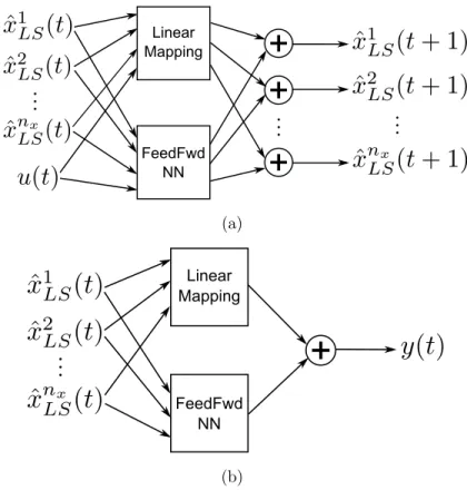
Figure 3 shows the considered model structure, for one input, one output
and nx states. Notice that the input and output signals of the benchmark
problem are one-dimensional, while the number of states nx is determined
by the order of the obtained BLA.
The first part of the model (Figure 3(a)) represents the state equation (1), with ˆx1
LS(t),xˆ2LS(t), . . . ,xˆ nx
LS(t) and u(t) as inputs, and ˆx1LS(t+ 1),xˆ2LS(t+
1), . . . ,xˆnx
LS(t+ 1) as outputs. Figure 3(b) instead shows the model used for
the output equation (2), where the states ˆx1
LS(t),xˆ2LS(t), . . . ,xˆ nx
LS(t) are the
inputs, and y(t) is the output signal.
Each NN block consists of the sum of sigmoid functions, characterized by three types of parameters, namely center position, width and amplitude. More details about the number of parameters in the model (coming from both linear and nonlinear terms) will be provided later in this section, when the obtained results will be discussed.
4.3. Identification of the BLA
Following the approach presented in Section 3, the first step towards the identification of the considered Wiener-Hammerstein system consists of obtaining a linear model that describes the input/output behavior.
The BLA is estimated following the Output Error approach (Ljung, 1999) on a part of the estimation data, namely using {u(t),y(t)}55000t=5001, excluding the first 5000 data points to eliminate transient effects. Different model orders have been tried out, by testing the performance of the resulting linear model on the remaining portion of the estimation set (used for validation).
Linear Mapping FeedFwd NN
+
+
+
(a) Linear Mapping FeedFwd NN+
(b)Figure 3: Model structure used to describe (a) the state equation, (b) the output equation,
for one input, one output and nx states. The feedforward NN block is added in parallel
to the linear model.
The best result in terms of RMSE is given by a 6th order model. The RMSE value obtained by this model on the test set is equal to 56.1 mV (the RMS value of the output signal is equal to 242.3 mV).
Figure 4 shows the error of the BLAeBLA(t) = y(t)−GˆBLA(u(t)) on the
test portion of the data set, together with the output values y(t).
In this way, matrices ˆA, ˆB and ˆC are obtained, and will be used in the next steps.
4.4. Approximation of the nonlinear states
Once the best linear model is available, an approximation of the nx = 6
nonlinear states can be obtained, as explained in Section 3.2. Here several
values (on a logarithmic scale) of λ were tried out, and an optimal value
0 20 000 40 000 60 000 80 000 -1.0 -0.5 0.0 0.5 Sample number Amplitude @ V D
Figure 4: Error obtained with the BLA - 6th order linear model - on the test set (gray), and measured output values (black).
æ æ æ æ æ æ à à à à à à 0.01 0.1 1 10 100 1000 0.030 0.035 0.040 0.045 Lambda value Validation RMSE
Figure 5: RMSE values on the validation data obtained by two initialized models, for
different choices of the trade-off parameterλ.
by the lowest RMSE on the validation data. Figure 5 shows an example in
which for every considered value of λ the RMSE obtained by two different
initialized models is reported.
4.5. Estimation of the nonlinear terms
In order to obtain good starting values for the model parameters, first the static problem (5-6) is solved, by using the measured input/output data, the approximate nonlinear states ˆxLS, and the estimated ˆA, ˆB and ˆC. The
model structure described above is used, by adding sigmoidal NN blocks in parallel to the linear model.
At this point the user needs to choose the structure of the NNs, in partic-ular the number of neurons in the hidden layer (i.e. the number of sigmoids that are summed up in the NN block) should be defined. Of course, this num-ber affects significantly the final numnum-ber of parameters in the model, that can explode if a high number of sigmoids is considered. Since by using the proposed initialization scheme model selection can be performed efficiently (as pointed out in Section 3.4), several number of sigmoids were tried out for f andg, and the resulting initialized nonlinear models were evaluated on the validation data set. The best trade-off between RMSE and number of
parameters in the model was obtained when choosing one sigmoid for f and
two sigmoids for g.
It can be shown that the number of model parameters (for f and g),
including both linear and nonlinear contributions, is given by the following formulas:
npar,f =nlin,f+nnl,f = ((nu+nx)·nx) + (nf ·(nu+nx+ 1) +nf ·nx+nx) npar,g =nlin,g+nnl,g = (nx·ny) + (ng·(nx+ 1) +ng·ny+ny)
where nu and ny are the number of inputs and outputs, nx is the number of
states, and nf and ng are the number of sigmoids used to describe the two
nonlinear terms in f and g respectively.
For the specific choice of nf = 1 and ng = 2, this results in:
npar,f = (1 + 6)·6 + 1·(1 + 6 + 1) + 1·6 + 6 = 62 (7) npar,g = 6·1 + 2·(6 + 1) + 2·1 + 1 = 23 (8)
which gives 85 model parameters in total.
The initialized model is then obtained by including again the recursion in the state equation, as already explained in Section 3.3.
The performance of the initialized model and of the final model obtained after optimizing all parameters are discussed in the next two subsections. 4.6. Results obtained with the initialized model
The obtained initialized model results in a RMSE value of 34 mV on the test set, to be compared with the 56.1 mV of the linear BLA model. Figure 6 shows the deviation of the estimated output values from the measured output values.
0 20 000 40 000 60 000 80 000 -1.0 -0.5 0.0 0.5 Sample number Amplitude @ V D
Figure 6: Error obtained with the initialized nonlinear model on the test set (gray), and measured output values (black).
It can be observed that the initialized nonlinear model does not signifi-cantly reduce the error, if compared with the BLA error in Figure 4, but it does capture some of the nonlinearity, since the asymmetric behavior that characterized the BLA error is partially removed.
4.7. Results obtained with the final fitted model
A Levenberg-Marquardt iterative search is then performed to optimize all 85 model parameters, starting from the parameters values of the initialized model. The search algorithm was let run for 300 iterations, since it was observed that the value of the cost function was decreasing slowly towards its (local) minimum. The RMSE obtained on the test set by the final fitted model is equal to 2.6 mV, a result that can be considered quite satisfactory when compared to other state-of-the-art methods (see later for comments on the use of the different techniques).
In Figure 7 a plot of the error obtained by the final fitted model is shown, together with the measured output values.
Compared with the error given by the initialized model in Figure 6, a significant improvement is observed after the optimization of the model pa-rameters.
The errors of the initialized model and of the final model are shown also in the frequency domain in Figure 8, together with the DFT spectrum of the modeled output.
It can be observed that in the pass band of the system the final model gives an error which is almost 20 dB lower than for the initialized model, but the gain is smaller at higher frequencies.
0 20 000 40 000 60 000 80 000 -1.0 -0.5 0.0 0.5 Sample number Amplitude @ V D
Figure 7: Error obtained with the fitted nonlinear model on the test set (gray), and measured output values (black).
0
5
10
15
-
100
-
80
-
60
-
40
-
20
0
Frequency
@
kHz
D
Amplitude
@
dB
D
Figure 8: DFT spectra of the modeled output (black), and of the errors of the initialized model (light gray) and of the final fitted model (dark gray) on the test set.
Model Estimation Test
BLA 55.3 56.1
Initialized nonlinear 33.2 34.0
Final nonlinear 2.6 2.6
Table 1: RMSE values (in mV) on estimation and test sets for the different models.
The results obtained with the different models on the estimation and test sets are summarized in Table 1.
4.8. Comments
Comparing the results obtained with the proposed approach with the ones given by the methods discussed in Section 2, it can be seen how a good trade-off is obtained between the achieved RMSE value and the number of parameters in the model.
A method that is fairly similar to the one presented in this paper is the polynomial nonlinear state-space model (Paduart et al., 2009), that resulted in very good RMSE results (0.42 mV), but where the final model was char-acterized by nearly 800 parameters (i.e. almost ten times more than for the model obtained in this work).
Other works that performed very well on the benchmark data (RMSE values ranging between 0.30 mV and 0.49 mV) made somehow use of the Wiener-Hammerstein structure (Sj¨oberg & Schoukens, 2011; Wills & Ninness, 2009; Lauwers, 2011) while for the algorithm presented here this was not necessary.
A last remark on the previous work by two of the authors on the bench-mark problem in (Marconato & Schoukens, 2009): the significant advantage provided with the method proposed in the present paper clearly shows the importance of addressing, in the identification procedure, both the nonlinear behavior of the system and the linear dynamics part. The improvement was only possible by adding explicitly the dynamics to the model.
5. Conclusion
In this paper a method for the identification of nonlinear state-space models, based on a combination of ideas from statistical learning and classic system identification, has been discussed. Thanks to the fact that system dynamics and nonlinear terms are identified separately, it is possible to solve an approximate version of the problem, making it possible to test efficiently several choices of nonlinear functions.
The proposed approach has been applied to the Wiener-Hammerstein benchmark problem. The obtained results are satisfactory, considering that no knowledge about the system was used in the identification procedure, and that the number of model parameters was kept very low.
6. Acknowledgements
This work is sponsored by the Fund for Scientific Research (FWOVlaan-deren), the Flemish Government (Methusalem Fund, METH1) and the
Bel-gian Federal Government (IAP VI/4).
References
Billings, S., & Fakhouri, S. (1982). Identification of systems containing linear
dynamic and static nonlinear elements. Automatica, 18, 15–26.
De Brabanter, K., Dreesen, P., Karsmakers, P., Pelckmans, K., De Brabanter, J., Suykens, J., & De Moor, B. (2009). Fixed-Size LS-SVM applied to the
Wiener-Hammerstein benchmark. In 15th IFAC Symposium on System
Identification. Saint-Malo, France.
Enqvist, M. (2005). Linear Models of Nonlinear Systems. PhD Thesis,
Link¨oping University, Sweden.
Falck, T., Pelckmans, K., Suykens, J., & De Moor, B. (2009). Identification of
Wiener-Hammerstein systems using LS-SVMs. In 15th IFAC Symposium
on System Identification. Saint-Malo, France.
Fletcher, R. (1987). Practical Methods of Optimization (2nd ed.). Wiley. Hastie, T., Tibshirani, R., & Friedman, J. (2009).The Elements of Statistical
Learning: Data Mining, Inference, and Prediction. Springer-Verlag. Hornik, K., Stinchcombe, M., & White, H. (1989). Multilayer feedforward
networks are universal approximators. Neural Networks,2, 359–366.
Lauwers, L. (2011). Some practical applications of the best linear approxima-tion in nonlinear block-oriented modeling. PhD Thesis, Vrije Universiteit Brussel.
Ljung, L. (1999). System Identification: Theory for the User (2nd ed.).
Prentice Hall, New Jersey.
Marconato, A., & Schoukens, J. (2009). Identification of
Wiener-Hammerstein benchmark data by means of Support Vector Machines. In 15th IFAC Symposium on System Identification. Saint-Malo, France. Paduart, J., Lauwers, L., Pintelon, R., & Schoukens, J. (2009). Identification
of a Wiener-Hammerstein system using the polynomial nonlinear state
space approach. In15th IFAC Symposium on System Identification.
Paduart, J., Lauwers, L., Swevers, J., Smolders, K., Schoukens, J., & Pin-telon, R. (2010). Identification of nonlinear systems using polynomial non-linear state space models. Automatica, 46, 647–656.
Pintelon, R., & Schoukens, J. (2012). System Identification: A Frequency Domain Approach. (2nd ed.). Wiley-IEEE Press.
Rugh, W. (1981). Nonlinear System Theory - The Volterra/Wiener
Ap-proach. The Johns Hopkins University Press, Baltimore.
Schoukens, J., Lataire, J., Pintelon, R., Vandersteen, G., & Dobrowiecki, T. (2009a). Robustness issues of the best linear approximation of a nonlinear
system. IEEE Trans. on Instrumentation and Measurement, 58, 1737–
1745.
Schoukens, J., Suykens, J., & Ljung, L. (2009b). Wiener-Hammerstein
bench-mark. In 15th IFAC Symposium on System Identification. Saint-Malo,
France.
Sj¨oberg, J., & Schoukens, J. (2011). The SYSID’09 benchmark problem:
a Wiener-Hammerstein model estimated from the best split of a linear model. Control Engineering Practice, (submitted to).
Suykens, J., Van Gestel, T., De Brabanter, J., De Moor, B., & Vandewalle,
J. (2002). Least Squares Support Vector Machines. World Scientific,
Sin-gapore.
Vapnik, V. (1998). Statistical Learning Theory. Wiley.
Verdult, V. (2002). Nonlinear System Identification: A State-Space
Ap-proach. PhD Thesis, University of Twente.
Wills, A., & Ninness, B. (2009). Estimation of generalised
Hammerstein-Wiener systems. In15th IFAC Symposium on System Identification.