http://siba-ese.unisalento.it/index.php/ejasa/index e-ISSN: 2070-5948
DOI: 10.1285/i20705948v10n1p1
A comparison study between three different Kernel estimators for the Hazard rate function By Salha, Rasheed
Published: 26 April 2017
This work is copyrighted by Universit`a del Salento, and is licensed un-der aCreative Commons Attribuzione - Non commerciale - Non opere derivate 3.0 Italia License.
For more information see:
DOI: 10.1285/i20705948v10n1p1
A comparison study between three
different Kernel estimators for the
Hazard rate function
Raid B. Salha
∗and Ali J. Rasheed
The Islamic University, Palestinian Territory, Occupied Department of Mathematics
Published: 26 April 2017
Kernel estimation is one of the most important data analytical tool, if we consider the non parametric approach in the estimation of the probability density function. In parallel, it is used to estimate the hazard rate function, which is one of the most important ways for representing the life time distri-bution in the survival analysis. As the support of the hazard rate function is in the non negative part of the real line [0,∞), its will be under the boundary effect near zero when the estimation is done using symmetric kernels such as the Gaussian kernel. Two kernel estimators for the hazard rate function were proposed using asymmetric kernels are the Reciprocal Inverse Gaussian and Inverse Gaussian kernel estimators to avoid the high bias near zero. In this paper, we conduct a theoretical comparison between those estimators by looking at their asymptotic bias, variance and the mean squared error. Also, a comparison of the practical performance of the three estimators based on simulated and real data will be present.
keywords: Inverse Gaussian kernel, reciprocal inverse Gaussian kernel, asymptotic bias, asymptotic variance, mean squared error.
1 Introduction
The hazard rate function is the instantaneous failure rate or (a force of morality), its represent the probability of failure between time x and x+ ∆, given that there were
∗
Corresponding author: [email protected]
c
Universit`a del Salento ISSN: 2070-5948
no failures up to time x. For more details see Cox and Oakes (1984). The hazard rate function is defined as follows:
Definition 1.1. The hazard rate function or age-specific failure rate, defined by:
r(x) = lim ∆−→0
P(x < X≤x+ ∆|x≤X)
∆ (1.1)
and by the definition of the conditional probability, we have
r(x) = f(x)
1−F(x) (1.2)
where f(x) is the pdf of the distribution and F(x) is the cdf.
LetX1, X2,· · · , Xna random sample from a distribution with an unknown probability density functionf satisfying the following assumptions:
(A1) The unknown density function f(x) has a continuous second derivativef(2)(x).
(A2) The bandwidth h=hn is a sequence of positive numbers and satisfies h→ 0 and
nh→ ∞asn→ ∞ .
(A3) The kernel K is a bounded probability density function of order 2 and symmetric about the zero.
Watson and Leadbetter (1964) has proposed the following kernel estimator for the hazard rate function.
Definition 1.2. The kernel estimator for the hazard rate function with bandwidth h is given by: ˆ r(x) = fˆ(x) 1−Fˆ(x) (1.3) where, ˆ f(x) = nh1 Pn i=1K x−Xi h , Fˆ(x) = nh1 Pn i=1 Rx 0 K x−Xi h
andK is bounded symmetric kernel function with R0∞K(u)du= 1.
Definition 1.3. The Gaussian kernel estimator for the hazard rate function rGˆ (x) is defined by: ˆ rG(x) = ˆ fG(x) ˆ SG(x) (1.4)
where, fˆG(x) and SˆG(x) are defined as follows:
ˆ fG(x) = nh1 Pn i=1KG x−Xi h , SGˆ (x) = 1−FGˆ (x) = 1−nh1 Pn i=1 Rx 0 KG u−Xi h du, where KG(x) is given byKG(x) = √1 2πe −x2 2 ,∀x∈ <.
Note that the support of the hazard rate function is in the non-negative part of the real line [0,∞), so when the estimation is based on symmetric kernels it will be under theboundary effect(calleda boundary biasproblem) near the zero. its causes that the estimator of the hazard rate function will take values outside the support.
To solve this problem, Chen (2000) has replaced the symmetric kernels by asymmetric Gamma kernel, which never assigns weight outside the support. Scaillet (2004) used this idea and proposed two new classes of density estimators, rely on the use of inverse Gaussian (IG) and the reciprocal inverse Gaussian (RIG) kernels in the place of the Gamma kernel. In Salha (2012), the estimation of the hazard rate function using theIG
kernel has been considered. In Salha (2013), the estimation of the hazard rate function using theRIGkernel has been considered.
Now, we state the following conditions under which, Scaillet (2004) has proposed theIG
and RIGkernel estimators of the pdf. Conditions
(C1) Let X1, X2,· · · , Xn be a random sample from a distribution with an unknown
probability density functionf defined on [0,∞), such thatf is twice continuously differentiable, andR∞
0 (x
3f00(x))2dx <∞.
(C2) h is a smoothing parameter satisfying h+nh1 →0 , and nh
5
2 →0, asn→ ∞.
Scaillet (2004) has proposed the followingIG kernel function as follows: Definition 1.4. TheIG kernel function is defined by :
KIG(x,1 h)(u) = 1 √ 2πhu3exp − 1 2hx u x −2 + x u ,u >0 (1.5) where h+nh1 →0 as n→ ∞ .
Using this kernel, Scaillet (2004) proposed the following IG kernel estimators of the pdf and cdf as follows:
Definition 1.5. TheIG kernel estimator of the pdf is defined by :
ˆ fIG(x) = 1 n n X i=1 KIG(x,1 h)(Xi) (1.6)
Definition 1.6. TheIG kernel estimator of the cdf is defined by :
ˆ FIG(x) = Z x 0 ˆ fIG(u)du= 1 n n X i=1 Z x 0 KIG(u, 1 h)(Xi)du. (1.7)
Using definitions 1.5 and 1.6, we propose the IGkernel estimator for the hazard rate function as follows:
Definition 1.7. TheIG kernel estimator for the hazard rate function is given by :
ˆ
rIG(x) =
ˆ
fIG(x)
Under the same conditions, Scaillet (2004) has proposed the following RIG kernel function.
Definition 1.8. TheRIG kernel function is defined by :
KRIG( 1 x−h, 1 h)(u) = 1 √ 2πhuexp −x−h 2h u x−h −2 + x−h u ,u >0 (1.9) where h+nh1 →0 as n→ ∞ .
Using this kernel, Scaillet (2004) proposed the following RIGkernel estimators of the pdf and cdf as follows:
Definition 1.9. TheRIG kernel estimator of the pdf is defined by :
ˆ fRIG(x) = 1 n n X i=1 KRIG( 1 x−h, 1 h)(Xi) (1.10)
Definition 1.10. TheRIG kernel estimator of the cdf is defined by :
ˆ FRIG(x) = Z x 0 ˆ fRIG(u)du= 1 n n X i=1 Z x 0 KRIG( 1 u−h, 1 h)(Xi)du. (1.11)
Using definitions 1.9 and 1.10, we propose the RIG kernel estimator for the hazard rate function as follows:
Definition 1.11. TheRIG kernel estimator for the hazard rate function is given by:
ˆ rRIG(x) = ˆ fRIG(x) 1−FˆRIG(x) . (1.12)
Salha (2012) and Salha (2013) studied the asymptotic properties for the estimators in Equations 1.8 and 1.12 such as the asymptotic normality, the strong consistency and investigated the optimal bandwidth that minimizes the mean squared error (M SE) and the asymptotic mean squared error (AM SE). In Section 2, we present a theoretical comparison between the three estimators from equations 1.4, 1.8 and 1.12. Also, a practical comparison between the three estimators to test their performance is given in Section 3. Finally, our conclusions will be given in Section 4.
2 A theoretical comparison
In this section, we make a brief theoretical comparison of the ˆrG(x), ˆrRIG(x) and ˆrIG(x) estimators by looking at their asymptotic bias, variance and the MSEs under the as-sumptionsA1,A2 andA3 for the Gaussian and under the conditionsC1 andC2for both
RIG and IG. Table 1 summarizes the results for the bias, variance and the MSEs for both ˆrRIG(x) and ˆrIG(x) are taken from Salha (2012) and Salha (2013).
The Estimator The Bias The Variance ˆ rG(x) f200S(x(x)h)2 +o(h) 2nh√f(x) πS2(x) +o( 1 nh) ˆ rIG(x) x 3f00(x)h 2S(x) +o(h) 1 2n√πhx −3 2 r(x) S(x)+o(n −1h−1 2) ˆ rRIG(x) xf 00(x)h 2S(x) +o(h) 1 2n√πhx −1 2 r(x) S(x)+o(n −1h−1 2)
Table 1: Summary for the Bias and Variance for the three estimators
2.1 The Bias
By looking to those expressions for the Bias in Table 1, we conclude the following re-marks:
1. Since the expressions of the Bias(ˆrRIG(x)) and Bias(ˆrG(x)) increases in xh and
h2 respectively, and hence near the zero (x∈(0, h)), we havexh < h2, which imply thatBias(ˆrRIG(x))< Bias(ˆrG(x)).
2. Bias(ˆrRIG(x)) and Bias(ˆrIG(x)) increases inxh and x3h respectively, and hence for any (x >1) we havexh < x3h, which imply thatBias(ˆrRIG(x))< Bias(ˆrIG(x)).
3. If 0 < x < 1 we have x3 < x and hence x3h < xh < h2 which imply that
Bias(ˆrIG(x))< Bias(ˆrRIG(x))< Bias(ˆrG(x)).
2.2 The Variance
By looking to the expressions for the Variance in Table 1, we conclude the following remarks:
1. The expressions of the V ar(ˆrRIG(x)) andV ar(ˆrG(x)) decreases in
√
xhand h re-spectively, and hence asx∈(0, h) we have√xh < h, which imply thatV ar(ˆrRIG(x))> V ar(ˆrG(x)).
2. The expressions of theV ar(ˆrRIG(x)) andV ar(ˆrIG(x)) decreases in
√
xhand√x3h respectively, and hence as 0 < x < 1 we have √xh > √x3h, which imply that
V ar(ˆrRIG(x))< V ar(ˆrG(x)).
3. The expressions of the V ar(ˆrRIG(x)) and V ar(ˆrIG(x)) decreases in
√
xh and √
x3h respectively, and hence as x > 1 we have √xh < √x3h, which imply that
V ar(ˆrRIG(x))> V ar(ˆrIG(x)).
2.3 The MSE
By Table 1, the squared bias for the RIG decreases if x ∈ (0, h) and hence as h de-creases we have squared bias for the RIG less than squared bias for Gaussian which imply that M SE(ˆrRIG(x)) < M SE(ˆrG(x)). A similar result hols for ˆrIG(x), we have
2.4 The Optimal AMSE
For any x ∈[0,∞), the optimal AMSE (AM SE∗) for the three estimators is the same and it is given by AM SE∗(ˆrRIG(x)) =AM SE∗(ˆrG(x)) =AM SE∗(ˆrIG(x)) = 5 4 f(x) 2√π 45 n−45f00(x) 2 5 S2(x) ! .
The AM SE∗(ˆrIG(x)) was driven in Salha (2012) and following the same techniques, we can derive the other two optimal AMSE. Now, we derive theAM SE∗(ˆrG(x)).
From Table 1, we have
M SE(ˆrG(x)) = f00(x)h2 2S(x) 2 + f(x) 2nh√πS2(x)+o(h 2) +o( 1 nh). (2.1)
Then under the conditions on the bandwidth h in C2 and as n → ∞, the AM SE is given by AM SE(ˆrG(x)) = f00(x) 2S(x) 2 h4+ f(x) 2n√πS2(x) h−1 (2.2)
To findAM SE∗(ˆrG(x)), the value of the optimal bandwidth, that minimizesAM SE(ˆrG(x)),
must be substituted in Equation (2.2).
Now, differentiate Equation (2.2) and equating it to zero, we obtain f00(x) S(x) 2 h3− f(x) 2n√πS2(x) h−2 = 0 (2.3)
Solve Equation (2.3) for h, we obtain the optimal bandwidth as follows:
h= f(x) 2n√π(f00(x))2 15 (2.4)
Now, substitute the value of the optimal bandwidth from Equation (2.4) into Equation (2.2), we get AM SE∗(ˆrG(x)) = f00(x) 2S(x) 2 f(x) 2n√π(f00(x))2 45 + f(x) 2n√πS2(x) f(x) 2n√π(f00(x))2 −15 (2.5) Now, by simplifying Equation (2.5), the following holds
AM SE∗(ˆrG(x)) = 5 4 f(x) 2√π 45 n−45f00(x) 2 5 S2(x) ! .
3 Practical Comparison
In this section, we compare between the three estimators of the hazard rate function by studying their performance using simulated and real data. The bandwidths has been chosen according to the following rules.
First, for the Gaussian estimator, the following rule from Silverman (1986) has been used to find the bandwidth
h∗ = 1.06ˆσn−15, (3.1) where, ˆ σ2 = 1 n−1 n X i=1 (xi−x¯)2.
and for theRIGandIGestimators, we used the bandwidth selection procedure that has been proposed by Scaillet (2004). This procedure indicates that iflnXfollows a normal distribution with parameters µ and σ2, then the optimal bandwidths for the RIG and
IG estimators are given respectively by
h∗∗= 16σ 5exp(1 8(−17σ 2+ 20µ)) 12 + 4σ2+σ4 !25 n−25, (3.2) and h∗∗∗= 16σ 5exp(1 8(17σ 2−20µ)) 12 + 68σ2+ 225σ4 !25 n−25, (3.3)
where, the unknown parameters σ and µare estimated as follows: 1. ¯x= 1nPn i=1lnxi , 2. ˆσ2= 1 n−1 Pn i=1(lnxi−x¯)2.
We use the S-Plus program in the implementation of those applications. 3.1 Simulation Studies
In this subsection, the performance of the three estimators are tested using simulation data from the exponential and normal distributions.
3.1.1 Simulation Study 1
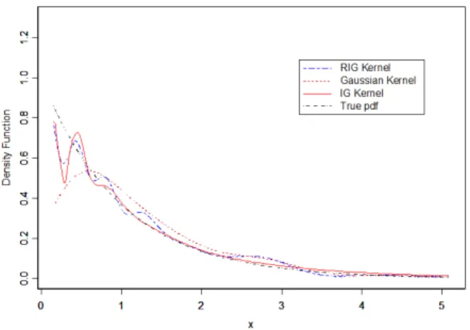
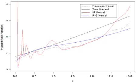
A sample of size 200 from the exponential distribution with pdff(x) =e−xis simulated. After that the density function and the hazard rate functions were estimated using the
RIG,IG and the Gaussian estimators. The estimated values and the true functions are plotted in Figure 1 and Figure 2, respectively. The two figures show that the performance of the RIG and IG estimator is better than that of the Gaussian estimator at the boundary near the zero. In the interior the behavior of the three estimators becomes more similar as we get away from the zero. Also theM SEfor the hazard rate estimators are listed in Table 2. Table 2 indicates that the RIGestimator has the smallestM SE.
M SE for the Estimators
M SE(ˆrRIG(x)) M SE(ˆrIG(x)) M SE(ˆrG(x))
0.4588251 0.4686859 0.4812027
Table 2:M SE of the hazard rate estimators for Simulation Study 1
Figure 1: The RIG,IG and Gaussian kernel estimators of the density function for the simulated data of the exponential distribution
Figure 2: The RIG,IG and Gaussian kernel estimators of the hazard rate function for the simulated data of the exponential distribution
3.1.2 Simulation Study 2
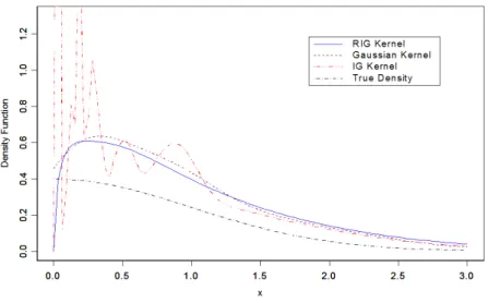
Two samples of size 40 and 100 from the normal distribution with pdf f(x) = √1 2πe
−x22
are simulated. After that the density function and the hazard rate functions were esti-mated using the RIG,IG and the Gaussian estimators. The estimated values and the true functions for the sample of size 100 are plotted in Figure 3 and Figure 4, respec-tively. The two figures show that the performance of the RIG estimator is better than that of the Gaussian and IG estimators at the boundary near the zero. In the interior the behavior of the three estimators becomes more similar as we get away from the zero. Also theM SE for the hazard rate estimators for the two samples are listed in Table 3. Table 3 indicates that the RIG estimator has the smallest M SE. From the results in Table 3, we note the performance of the three estimators for large sample is better than that for the small sample.
M SE for the Estimators
Sample size M SE(ˆrRIG(x)) M SE(ˆrIG(x)) M SE(ˆrG(x))
40 0.3432449 0.62093 0.6671531
100 0.0412683 0.2949743 0.1256913 Table 3:M SE for the hazard rate estimators for Simulation Study 2
Figure 3: The RIG,IG and Gaussian kernel estimators of the density function for the simulated data of the normal distribution
Figure 4: The RIG,IG and Gaussian kernel estimators of the hazard rate function for the simulated data of the normal distribution
3.2 Real Data
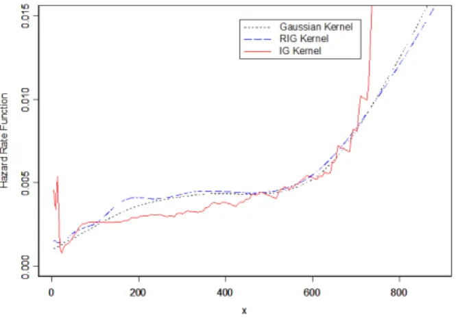
We use the survival time of the lung cancer patients given in data from a study of lung cancer patients conducted by the North Central Cancer Treatment Group, see Loprinzi et al. (1994), to exhibit and compare the practical performances of the Gaussian, RIG
andRIGestimators. We exclude thecensored data(means some individuals may not observed for the full time to failure which for example stay alive at the end of the study or may leave the study before they die ), so here we assume that the applications done using a complete study (without censoring). The data gives the lengths of the treatment spells (in days) of control patients were hospitalized. The objective is to estimate the hazard rate function which in this case represents the instant potential per unit of time that an individual die within the time interval (x, x+ ∆) given that it was known to be alive up to timex.
Figure 5 and Figure 6 show the estimators of the probability density and hazard rate function, respectively. Although the suggested values of the density and hazard rate functions from the estimators are different, they suggest a similar structure for the esti-mated functions. As we see, the divergence of the estimators gets large at the boundary near the zero and becomes smaller in the interior especially from approximatelyx≥200.
Figure 5: The RIG,IG and Gaussian kernel estimators of the density function for the survival time of the lung cancer patients
Figure 6: The RIG,IG and Gaussian kernel estimators of the hazard rate function for the survival time of the lung cancer patients
4 Conclusion
In this paper, we compared between three kernel estimators for the hazard rate function, the RIG, IG and the Gaussian estimators. A theoretical comparison between those estimators based on comparing the asymptotic biases, variances and mean squared error indicated that the two asymmetric kernel estimators (ˆrIG and ˆrRIG) are better than the Gaussian at the boundary near the zero. This result leads to deduce that the mean squared errors for both (ˆrIGand ˆrRIG) are less than that of the Gaussian kernel estimator
(ˆrG) because its based on symmetric kernel. Also, the practical comparison between the three estimators using simulation studies and real data indicated that the performance of the asymmetric kernel estimators (ˆrIG and ˆrRIG)is better than that of ˆrG, especially
near the zero, confirming the previous theoretical discussion.
In this paper, we presented three estimators of the hazard rate function and compared between them theoretically and practically. The main idea was to replace the symmetric kernel function by asymmetric kernel functions to avoid the boundary bias problem near the zero, when estimating the hazard rate function. To increase the accuracy of these estimators, we suggest to use a variable bandwidth that depends on the points where we estimate the hazard rate function. This variable bandwidth together with the asymmetric kernel will increase the performs of the kernel estimators of the hazard rate function.
References
Chen, S. X. (2000). Probability density function estimation using gamma kernels.Annals of the Institute of Statistical Mathematics, 52(3):471–480.
Cox and Oakes (1984). Analysis of survival data. Champion and Hall.
Loprinzi, C. L., Laurie, J. A., Wieand, H. S., Krook, J. E., Novotny, P. J., Kugler, J. W., Bartel, J., Law, M., Bateman, M., and Klatt, N. E. (1994). Prospective evaluation of prognostic variables from patient-completed questionnaires. north central cancer treatment group. Journal of Clinical Oncology, 12(3):601–607.
Salha, R. (2012). Hazard rate function estimation using inverse gaussian kernel. The Islamic university of Gaza journal of Natural and Engineering studiesl, 20(1):73–84. Salha, R. (2013). Estimating the density and hazard rate functions using reciprocal
inverse gaussian kernel. InProceedings of the 15th international conference of Applied Stochastic Models and Data Analysis (ASMADA), pages 759–766. ASMADA.
Scaillet, O. (2004). Density estimation using inverse and reciprocal inverse gaussian kernels. Communications in Statistics Theory and Methods, 16:217–226.
Silverman, B. W. (1986). Density estimation for statistics and data analysis, volume 26. CRC press.