Australia
Department of Econometrics
and Business Statistics
http://www.buseco.monash.edu.au/depts/ebs/pubs/wpapers/
Semiparametric estimation of the dependence parameter of
the error terms in multivariate regression
Gunky Kim, Mervyn J. Silvapulle and Paramsothy Silvapulle
February 2007
Semiparametric estimation of the dependence
parameter of the error terms in multivariate regression
By GUNKY KIM, MERVYN J. SILVAPULLE, AND PARAMSOTHY SILVAPULLE
Department of Econometrics and Business Statistics, Monash University, P.O. Box 197, Caulfield East, Melbourne, Australia 3145.
[email protected], [email protected], [email protected]
First version: Presented at the Joint Statistical Meetings, Minneapolis, August 2005. Second version: August 2006.
Summary
A semiparametric method is developed for estimating the dependence parameter and the joint distribution of the error term in the multivariate linear regression model. The nonpara-metric part of the method treats the marginal distributions of the error term as unknown, and estimates them by suitable empirical distribution functions. Then a pseudolikelihood is maximized to estimate the dependence parameter. It is shown that this estimator is as-ymptotically normal, and a consistent estimator of its large sample variance is given. A simulation study shows that the proposed semiparametric estimator is better than the para-metric methods available when the error distribution is unknown, which is almost always the case in practice. It turns out that there is no loss of asymptotic efficiency due to the estimation of the regression parameters. An empirical example on portfolio management is used to illustrate the method. This is an extension of earlier work by Oakes (1994) and Genest et al. (1995) for the case when the observations are independent and identically distributed, and Oakes and Ritz (2000) for the multivariate regression model.
Some key words: Copula; Pseudolikelihood; Robustness.
1. Introduction
Estimation of the joint distribution of a random vector and learning about inter-dependence among its components are important topics in statistical inference. This paper develops a method for estimating the joint distribution and the dependence parameter of the error distribution in multivariate linear regression.
It is now well-known that the joint cumulative distribution function H(x1, . . . , xk) of
a random vector (X1, . . . , Xk) with continuous marginals Fi(xi) = pr(Xi ≤ xi) has the
unique representation H(x1, . . . , xk) = C{F1(x1), . . . , Fk(xk)}, where C(u1, . . . , uk) is the
joint cumulative distribution of (U1, . . . , Uk) and Ui = Fi(Xi) is distributed uniformly on
[0,1],i= 1, . . . , k (Sklar (1959)). The functionC is called the copula of (X1, . . . , Xk). There
has been a substantial interest in the recent literature on copulas for studying multivariate observations. Two of the reasons for such increased interest includes the flexibility it offers because it can represent practically any shape for the joint distribution, and its ability to separate the intrinsic measures of association between the components of the random vector from the marginal distributions.
It is possible that distribution functions H, F1, . . . , Fk,and C may belong to parametric
families, for example, H(x1, . . . , xk;α1, . . . , αk, θ) =C{F1(x1;α1), . . . , Fk(xk;αk);θ}. In this
case, θ is called the dependence parameter or association parameter. This helps to separate the marginal parameters from the intrinsic association which is captured byθ.An attractive feature of this approach is that the copula C and the association parameter θ are invariant under continuous and monotonically increasing transformations of the marginal variables. Hence copulas have an advantage when the interest centers on intrinsic association among the marginals (Wang and Ding (2000), Oakes and Wang (2003)).
Copulas have been used in a very wide range of applied areas and the literature is quite ex-tensive indeed. The areas include survival analysis, analysis of current status data, censored
data and finance (Bandeen-Roche and Liang (2002), Wang (2003), Wang and Ding (2000), Shih and Louis (1995), and Cherubini et al. (2004)). Joe (1997) provides a comprehensive and authoritative account of statistical inference in copulas and dependence measures using copulas. Hutchinson and Lai (1990) provides an extensive range of practical examples where copulas are useful. In what follows, we shall restrict our discussion to bivariate observations only, for simplicity. However, the extensions to higher dimensions would be straight forward. The use of Copulas in risk management has been increasing substantially in the recent past where the main interest is on the whole distribution rather than just the association parameter (Cherubini et al. (2004)). As an example, let Y1 and Y2 denote the market
values of two shares, say a bank and a mining company respectively. Let x denote a market index such as the Dow Jones Index. Suppose that Y1 = xT1β1 +²1 and Y2 = xT2β2 +²2,
where x1 = x2 = (1, x)T. Thus, after accounting for the overall market movements, ²1 and ²2 represent the risks that are not under the control of the investor. For managing the risks
associated with a portfolio consisting of these two investments, for example, for assessing the need for diversification of investments, the main quantities of interest are functions of the joint distribution of (²1, ²2). Examples of quantities that are of interest include, (i)
pr(Y1 ≤a1 and Y2 ≤a2) and pr(Y1 ≤a1 |Y2 ≤a2),where a1 and a2 are given numbers, and
(ii) theValue at Risk, c, defined by pr{b1Y1+ (1−b1)Y2 ≤c} ≤α, where α is a given small
number, for example α = 0.05, andb1 is the proportion of investment in the first asset.
This paper develops a new semiparametric method for estimating the dependence para-meterθ and joint distribution of the error term, (²1, ²2).If the assumptions for the traditional
normal-theory linear model are satisfied, then it would be possible to obtain an optimal esti-mate of the joint distribution of the error terms by maximum likelihood. However, in many areas of applications, for example risk management, the marginal distributions of the error terms are far from being normal. In fact, returns from investments are notorious for being
long-tailed and skewed. Further, the marginal distributions of (²1, ²2) may also take different
functional forms. For example, ²1 and ²2 may be distributed as gamma and normal
respec-tively. Consequently, the well known elliptically symmetric families of distributions, such as the multivariate normal and t, are inadequate. Further, often it is of interest to apply inference methods that make as few assumptions as possible about the functional form of the distribution. In this paper, we propose a semi-parametric method that fits this requirement. An attractive feature of this method is that it does not cause any additional difficulties due to the marginal distributions being long tailed and skewed, features that are common in financial data and have attracted considerable interest in financial statistics.
The method introduced in this paper started with Oakes (1994) and Genest et al. (1995). They proposed a procedure for estimating the dependence parameter in a copula for inde-pendent and identically distributed observations when the marginal marginal distributions are treated as unknown. The method involves two stages of estimation: In the first stage, the marginal distributions are estimated by their respective empirical distribution functions, and in the second stage, the maximum likelihood is applied with the marginal distributions replaced by the corresponding empirical distributions. Genest et al. (1995) showed that this estimator is asymptotically normal for different settings; see also Wang and Ding (2000) and Shih and Louis (1995). In this paper, we extend this approach to the multivariate linear regression model when the interest is centered on the joint distribution of the multivariate error term. Oakes and Ritz (2000) also studied estimation of the copula of the error term in the same multivariate linear regression setting but they used a fully parametric approach.
Now, to introduce the method developed here, let us consider the bivariate investment example considered earlier in this section. Let F1(t1) = pr(²1 ≤ t1), F2(t2) = pr(²2 ≤ t2)
and let C(u1, u2;θ) denote the copula of (²1, ²2), θ being an unknown parameter which we
given by pr(²1 ≤ t1, ²2 ≤ t2) = C{F1(t1), F2(t2);θ}. Throughout, we shall assume that
the functional form of C(u1, u2;θ) is known, but F1 and F2 are unknown. We propose an
estimator of θ and show that it is consistent and asymptotically normal. Further, we also obtain a consistent estimator of its asymptotic variance so that confidence intervals may be constructed. Simulation results show that our proposed method performs better than the traditional fully parametric methods of inference when the functional forms of the marginal distributions are unknown, which is of course almost always the case.
The rest of the paper is structured as follows. In the next section, we state the estimation method more formally. Section 3 presents simulation results to illustrate the superiority of the semiparametric method when the marginal distributions are unknown. Section 4 illustrates the method using a data example. Section 5 concludes. The proofs are given in appendix.
2. The main results
As indicated in the introduction, we shall consider the bivariate case for notational sim-plicity. The extension to the multivariate case is almost straight forward. Let the data generating process for (Y1, Y2) be Y1 =xT1β1+²1, and Y2 =xT2β2+²2 where x1 and x2 are
vectors of covariates associated with Y1 and Y2 respectively. In what follows, these
covari-ates are assumed to be non-stochastic. However, the results would hold, with appropriate modifications, even if they are stochastic. Suppose that there are n independent obser-vations (Y1i, x1i, Y2i, x2i), (i = 1, . . . , n). Thus, we have Ypi = xTpiβp +²pi, (i = 1, . . . , n,
p = 1,2). Let fp and Fp denote the probability density and cumulative distribution
func-tions of ²p respectively, p = 1,2. Let C(u1, u2;θ) and c(u1, u2;θ) denote the copula of
(²1, ²2) and the corresponding density function, respectively. Then, the loglikelihood takes
the form, `∗(θ, β
P
logc{F1(²1i), F2(²2i);θ}andB(β1, β2, f1, f2) =
P
log{f1(²1i), f2(²2i)}.The maximum
like-lihood estimator of (θ, β1, β2) is simply the point at which`∗(β1, β2, θ) reaches its maximum.
If the joint distribution of (²1, ²2) is correctly specified then this estimator is consistent and
asymptotically normal, provided some regularity conditions are satisfied. Since the term
B(β1, β2, f1, f2) does not depend on θ, it may be ignored for the purposes of estimatingθ by
maximum likelihood.
Now, we introduce the following semiparametric estimator of the copula parameter θ, when (F1, F2) is unknown:
(a) Let ˜βp be an estimatorβp such that n1/2(ˆβ
p−βp) =Op(1), for p= 1,2.
(b) Compute the residuals ˜²pj =ypj−xTpjβ˜p, for p= 1,2 and j = 1, . . . , n.
(c) Estimate Fp(t) by ˜Fpn(t) defined by ˜Fpn(t) = {1/(n+ 1)}Σni=1I(˜²pi ≤ t), where I is the
indicator function; thus ˜Fpn is the empirical distribution of {˜²p1, . . . ,˜²pn}, except for the
denominator (n+ 1) instead ofn.
(d) Estimate θ by ˜θ, defined by ˜θ = argmaxθ L(θ) where
L(θ) = Σ logc{F˜1n(˜²1i),F˜2n(˜²2i);θ}.
This four-step procedure reduces to that proposed by Oakes (1994) and Genest et al. (1995) for the case when (Y1i, Y2i) are independent and identically distributed fori= 1, . . . , n.
Since ( ˜F1n,F˜2n) is expected to be close to (F1, F2) for largen, it is reasonable to expect that
the foregoing estimator is likely to be a reasonable estimator.
We will show that ˜θ is consistent and asymptotically normal, and obtain a closed form expression for the asymptotic variance. By substituting sample estimates for the asymptotic variance formulae, we shall obtain a consistent estimator of the large sample variance.
While the idea that underlies our new method is intuitively simple and is a natural extension of Oakes (1994) and Genest et al. (1995), the mathematical arguments to derive
its essential properties are quite involved. Therefore, in this section we shall indicate the main ideas in a simple form and relegate the rigorous details to an appendix. Even there, only the main steps are indicated. More detailed and rigorous proofs are given in a working paper of the authors at Monash University.
To indicate the general approach, let l(θ, u1, u2) = log{c(u1, u2;θ)}, and let l with
sub-scripts θ, 1, and 2 denote partial derivatives with respect to θ, u1 and u2 respectively. For
example, lθ(θ, u1, u2) = (∂/∂θ)l(θ, u1, u2) and lθ,1(θ, u1, u2) = (∂2/∂u1∂θ)l(θ, u1, u2). Now,
let us first expand L(˜θ) in Taylor series about the true value θ0.
0 = (∂/∂θ)L(˜θ) = (∂/∂θ)L(θ0) + (˜θ−θ0)(∂2/∂θ2)L(θ0) + (1/2)(˜θ−θ0)2(∂3/∂θ3)L(θ∗)
where θ∗ lies in the line segment [θ
0,θ˜]. Now, solving this for n1/2(˜θ−θ0), we have that n1/2(˜θ−θ 0) =An/(Bn+Cn) (1) where An =n−1/2Σin=1lθ{θ0,F˜1n(˜²1i),F˜2n(˜²2i)}, (2) Bn =−n−1Σin=1lθ,θ{θ0,F˜1n(˜²1i),F˜2n(˜²2i), (3) Cn =−(˜θ−θ0)[(2n)−1Σni=1lθ,θ,θ{θ∗,F˜1n(˜²1i),F˜2n(˜²2i)}]. (4)
The main reasons for the technical details leading to the asymptotic properties of ˜θ turns out to be complicated are that the expressions in (2)- (4) are sums of dependent random variables and ˜Fpn(˜²pi) is a non-smooth function. The dependence of the random variables
will be dealt with by using results for U-statistics and multivariate rank order statistics. To deal with the non-smoothness due to the presence of ˜Fpn, results for weighted empirical
processes in Koul (2002) will be used.
By essentially mimicking the arguments in section 6.4 of Lehmann (1983), it can be shown that the estimator ˜θ is consistent. To establish the asymptotic normality of n1/2(˜θ−θ
consider the behaviour of the terms in (2) - (4). We will show that{F˜1n(˜²1i),F˜2n(˜²2i)} in (3)
can be approximated by {F1(²1i), F2(²2i)} so that Bn =−n−1Σni=1lθ,θ{θ0, F1(²1i), F2(²2i)}+
op(1), which converges to γ in probability, where
γ =E£¡lθ{θ0, F1(²1), F2(²2)}
¢2¤
. (5)
By assuming that the third order derivatives lθ,θ,θ are bounded by integrable functions in a
small neighbourhood of θ0, we have n−1Σni=1lθ,θ,θ{θ∗,F˜1n(˜²1i),F˜2n(˜²2i)} = Op(1) and hence
Cn = op(1). Therefore, Bn+Cn converges to γ in probability. To obtain the asymptotic
distribution of An in (2), we approximate ˜Fpn by Fpn, the empirical distribution of the
unobserved error terms rather than by its true population distribution Fp, (p= 1,2). This
leads to An =An1+op(1), where An1 =n−1/2Σni=1lθ{θ0, F1n(²1i), F2n(²2i)}. It may be noted
that An1 is a multivariate rank order statistic of the form n−1ΣJ{F1n(²1i), F2n(²2i)} for
some functionJ. The asymptotic distribution of such general rank order statistics have been studied extensively in the literature, for example see R¨uschendorf and Ruschendorf (1976) and Ruymgaart et al. (1972). The asymptotic distribution of the foregoing particular form of An1 was obtained by Genest et al. (1995). Applying Proposition 2.1 therein, we have
that An1 converges in distribution to N(0, σ2), where σ2 = var£l θ{θ0, F1(²1), F2(²2)}+W1(²1) +W2(²2) ¤ , (6) Wp(²p) = Z Z I¡Fp(²p)≤up ¢ lθ,p{θ0, u1, u2}c(u1, u2;θ)du1du2, p= 1,2. (7)
Thus, we conclude thatn1/2(˜θ−θ
0) converges in distribution toN(0, ν2),whereν2 =σ2/γ2.
To obtain an estimate of the asymptotic variance ν2, we estimate σ2 and γ2 separately.
By substituting estimated quantities to the unknown quantities in (5), an estimate of γ2 is
˜
γ =−n−1Σn
i=1lθ,θ{θ,˜ F˜1n(˜²1i),F˜2n(˜²2i)}. (8)
Since σ2 = var{T(θ
cannot be observed, we estimate σ2 by the sample variance
˜
σ2 = Sample variance of ˜T
1(˜θ), . . . ,T˜n(˜θ), (9)
of the pseudo observations, ˜
Ti(θ) =lθ{θ,F˜1n(˜²1i),F˜2n(˜²2i)}+ ˜W1(˜²1i, θ) + ˜W2(˜²2i, θ), i= 1, . . . , n, (10)
where W˜p(t, θ) = n−1Σnj=1I(t≤˜²pj)lθ,p{θ,F˜1n(˜²1j),F˜2n(˜²2j)}, p= 1,2. (11)
This leads to the consistent estimator ˜ν2 = ˜σ2/s˜2 forν2.Now, let us state the main theorem.
A set of regularity conditions to ensure that the theorem holds, is stated in the Appendix where the proof of theorem is also given.
Theorem 0.1. Assume that the regularity conditions given in the Appendix hold. Then, the
semiparametric estimator θ˜is a consistent estimator ofθ0 and the asymptotic distribution of n1/2(˜θ−θ
0) is N(0, ν2), where ν2 =σ2/γ2. Further, a consistent estimator ν˜2 of ν2 is given by ν˜2 = ˜σ2/γ˜2, where σ˜2 and ˜γ are as in (9) and (8) respectively.
The expression for the asymptotic variance of n1/2(˜θ−θ
0) is the same as that for the
case when the there is no regression structure and the observations are independent and identically distributed. Therefore, Proposition 2.2 of Genest et al. (1995) is applicable to the setting in the above theorem as well. In particular, the semiparametric estimator ˜θ is fully efficient for the independent copula, otherwise there is a loss of asymptotic efficiency due to the marginal distributions being unknown.
The parameterθcan be estimated by other methods as well. The two main ones that play central roles in inference for copulas are the maximum likelihood and the inference function for margins (see Joe (1997)). Both of these are fully parametric. Let Fp(t;αp) denote the
distribution of the error term ²p for every p. Now the loglikelihood takes the form
where B(β1, β2, α1, α2) =
P
log{f1(²1i, α1) f2(²2i, α2)} and L(θ, β1, β2, α1, α2) =
P
logc{F1(²1i, α1), F2(²2i, α2);θ}.
The maximum likelihood estimator of (θ, β1, β2, α1, α2) is simply the maximizer of `(θ, β1, β2, α1, α2).The method of maximum likelihood for copulas is usually not the preferred
one due to difficulties such as multiple maxima for the likelihood and erratic behaviour of the estimator. The inference function method has been proposed as a close alternative - see Joe (1997) for a thorough account of this topic. In this method, the model is estimated in two stages. In the first stage, the parameter (βp, αp) is estimated using the data for the pth
margin, for everyp; let this estimator be denoted by (ˆβp,αˆp).Then, in the second stage,θ is
estimated by maximizing the likelihood function with (βp, αp) replaced by its estimator (p=
1,2). Thus, the inference function for margins estimator ofθ isargmaxθ `(θ,βˆ1,βˆ2,αˆ1,αˆ2).
One would expect that the maximum likelihood and the inference function for margins methods are likely to be non-robust against misspecification of the marginal distributions. The simulation results in section 4 illustrate that the semiparametric method is considerably better than the maximum likelihood and inference function for margins method when the form of the marginal distributions are unknown, which is almost always the case in practice.
3. Simulation study
We carried out a simulation study to compare the semiparametric method with its com-petitors, the maximum likelihood and inference function for margins, and also to evaluate the reliability of the large sample confidence interval for θ given in Theorem 1.
Design of the simulation study
The following five copulas were considered in the study. More details about them may be found in Joe (1997) and Nelsen (1999).
(2) Frank copula: C(u, v;θ) = −θ−1log¡[1 + (e−θu−1)(e−θv −1)]/(e−θ−1)¢
(3) Gumbel copula: C(u, v;θ) = exp−¡(−logu)θ+ (−logv)θ¢1θ
(4) Joe copula: C(u, v;θ) = 1−¡(1−u)θ+ (1−v)θ−(1−u)θ(1−v)θ¢1θ
(5) Plackett copula:
C(u, v;θ) = [1 + (θ−1)(u+v)− {{(1 + (θ−1)(u+v)}2−4θ(θ−1)uv}12]/{2(θ−1)}.
These copulas cover a very wide range of distributional shapes. The maximum likelihood and inference function for margins estimators that are used in this simulation study assumed that the marginal distributions were normal. The following sets of marginal distributions were considered: (1) X1 and X2 are normally distributed, (2) X1 ∼ tr and X2 ∼ tr, (3)
X1 ∼ tr and X2 ∼ skew tr with skewness = 0.5, and (4) X1 ∼ tr and X2 ∼ χ22. The first
one corresponds to the correct specification of the marginal distributions, while each of the others leads to a misspecification of the model. A skew tr-distribution has tails that are
of the same order as that for tr but the probability masses on either sides of the origin
are different, leading to skewness. The values 3 and 8 were considered for the degrees of freedom r of the tr-distribution. Since the semiparametric method estimates each marginal
distribution nonparametrically, it is meant to be used when the sample size is moderate to large. In this study, we considered sample sizes ranging from 50 to 1000. This captures a broad range of realistic settings.
All the computations were programmed in MATLAB Version 7.0.4. Optimizations were performed using the procedure ”fmincon.m” in the ”Optimization Toolbox (3.0.2).
Results:
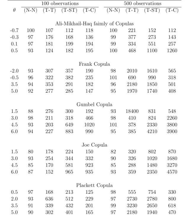
Only a selection of the simulation results are presented here to save space. Overall, the difference between the inference functions for margins and maximum likelihood estimators were small, with the former performing slightly better. Therefore, the results for maximum likelihood are not presented here.
——— Tables 1-2 about here
————-Each marginal distribution is correctly specified as normal: The results are given in Table 1 under the heading N-N. Since the marginal distributions and the copula are correctly specified, there is no mis-specification. Thus, as expected, the inference function for mar-gin estimators perform slightly better than the semiparametric estimator. However, the differences are small.
Each marginal distribution is incorrectly specified as Normal:
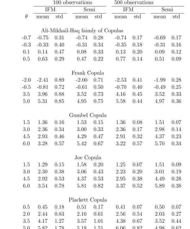
Table 2 provides estimated bias computed as the mean of the simulated estimates of θ
minus the true value ofθ.The same table also provides standard deviations of the simulated estimates of θ. Table 2 shows quite clearly that (i) the maximum likelihood and inference function for margin estimators are highly nonrobust against misspecification of the marginal distributions, and (ii) the distribution of the semiparametric estimator is centered around the true value of θ and is far superior to the maximum likelihood and the inference function for margin estimators ofθ.We recognize that the very large values for relative MSE in Table 1 are not precise, but we presented them because they convey the message that misspecification of the marginal distribution may cause the parametric estimators to be biased and the standard deviation of the estimators could become relatively unimportant compared to the bias.
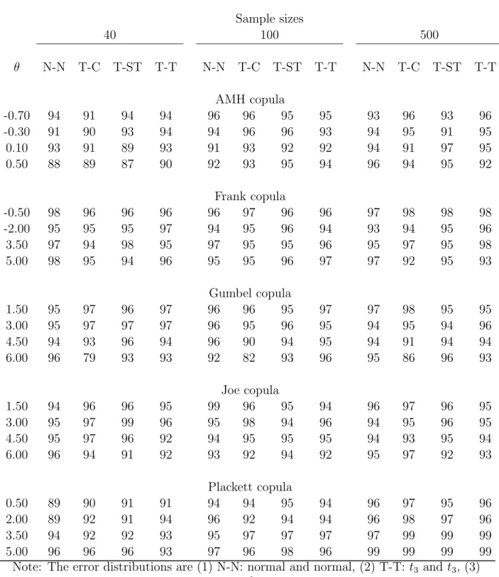
Table 3 shows that an approximate 95% confidence interval based on a normal approx-imation for the large sample distribution of ˜θ, has coverage rates close to 95% for sample size ≥ 40. In some isolated cases, it dropped to a rate just below 90 %. These results show that the semiparametric method also offers a reliable and easy to compute large sample confidence interval for θ.
4. An illustrative example
To illustrate the semiparametric method, we discuss an example that is very similar to that we discussed in the Introduction. The response variables are returns on shares of ANZ Bank and of BHP-Billiton. We consider regression of these variables on the All Ordinaries Index (Australia), a market index similar to the Dow Index in the USA. The variables are defined as follows: y1t = ln(At/At−1)−ln(Tt/Tt−1), y2t = ln(Bt/Bt−1)−ln(Tt/Tt−1), zt=ln(It/It−1)−ln(Tt/Tt−1),where At= ANZ price index, Bt = BHP-Billiton price index,
Tt = 90-day Treasury bill rates, and It = All Ordinaries Index. We used monthly data for
the period July 1981 to July 2001.
We consider the regression model, Ypt = xTtβp +²pt, p = 1,2, where xt = (1, zt)T. In
the first stage, we estimated β1 and β2 by least squares. The estimated models are, y1t =
−0.064 + 0.840zt+ ˜²tand y2t =−0.470 + 0.992zt+ ˜²t,respectively. Then we considered
Ali-Mikhail-Haq, Clayton, Gumbel, Joe, and Independent copulas for the joint distribution of the error term, (²1, ²2).Closed form expressions for the copulas were given in the previous section.
We assessed the goodness of fit using the chi-square statistic with a grid of 20 cells. Since the models are nonnested and method is semiparametric, the distribution theory of the chisquare statistic is not available. However, it is reasonable to compare the chi-square statistics. Based on such diagnostics, we concluded that a Gumbel copula provided the best fit for the joint distribution of the error terms, although some of the others were not too different. The estimated value of the Gumbel copula parameter is ˜θ = 1.076 and the standard error = 0.046. Hence, an estimate of the joint distribution of (²1, ²2) is C( ˜F1(²1),F˜2(²2); 1.076), and
an estimate of the joint distribution of (y1, y2) conditional onx is
C{F˜1{y1−(−0.064 + 0.840z)},F˜2{y2−(−0.470 + 0.992z)}; 1.076], (12)
where ˜F1 and ˜F2 are the empirical distributions of the residuals of the error terms in the two
associated with risk. For example, it can be used to estimate (i) the probability of the random components of returns, namely²1 and²2,falling belowa1 anda2 respectively where a1 anda2 are given, (ii) the probability, pr(Y1 ≤a1, Y2 ≤a2 | z),of the returns falling below a1 and a2 for a given value of the explanatory variable z, and (iii)Value-at-Risk c of the
portfolio w = b1Y1 + (1−b1)Y2, defined by pr{b1Y1+ (1−b1)Y2 ≤ c | z} ≤ α, where α is
a given small number, for example α = 0.05, and b1 is the proportion of investment in the
first asset.
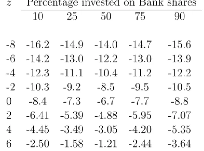
As an example, Table 4 provides estimates of Value-at-Risk of the portfolio for several values ofb1 and z. This is very similar to those for the example on pages 68-69 in Cherubini
et al. (2004). Table 4 shows that as the proportion b1 moves closer to 50%, the
Value-at-Risk decreases indicating that portfolio diversification reduces risk, and the rate at which the Value-at-Risk decreases is indicative of the effectiveness of diversification on reducing risk. Table 4 also shows that the Value-at-Risk is almost symmetric about b1 = 50%, which
is consistent with our observation that the histograms, not given here, of the regression residuals for the two assets appear to have approximately equally heavy tails.
The chi-square goodness fit statistics for a 5 by 4 grid, turned out to be 5.2 and 380 for the semiparametric method and for the inference function for margins method with normal distribution for each margin, respectively. Therefore, the the former method provided a significantly better fit than the latter one.
5. Conclusion
We extended a semiparametric estimator of Oakes (1994) and Genest et al. (1995) for estimating the dependence parameter and the joint distribution of the error terms of the multivariate linear regression model. We showed that this estimator is asymptotically nor-mal. It turns out that the form of the asymptotic variance is very similar to that obtained
by Genest et al. (1995) for the case when the observations are independent and identically distributed. This helped us to use his results and construct consistent estimates for the as-ymptotic variance and confidence interval for the dependence parameter. Simulation results showed that our semiparametric estimator performs better than the parametric ones when true error distribution deviates from that assumed by the parametric methods, maximum likelihood and inference function for margins. Further, the semiparametric method is fully efficient for the independent copula, which extends a result of Genest et al. (1995) for case of independent and identically distributed observations. Since the form of the expression for the asymptotic variance of the semiparametric estimator is very similar to that when the ob-servations are independent and identically distributed, we would expect that the conditions in Genest and Werker (2002) for the semiparametric estimator to be efficient are also likely to be applicable in the regression case as well.
Acknowledgment
Appendix: Proofs
Here we shall indicate the main steps in the proof of Theorem 1. A more detailed proof is provided in an unpublished manuscript. As in the text, the index p refers to the pth component,p= 1,2; for simplicity we shall avoid writing ‘for every p’ or ‘p= 1,2’, as far as possible. Let H(θ, u1, u2) denote a derivative ofl(θ, u1, u2) up to third order in θ and second
order in (u1, u2), and let (U1, U2) denote a random variable with the same distribution as
(F1(²1), F2(²2)) so that (U1, U2) ∼ C(u1, u2;θ0). Now, let us introduce the regularity
condi-tions.
Condition C:
(C.1): The distribution function Fp has continuously differentiable density, denoted by fp
and it satisfies kfpk∞ <∞ and
° °f0 p ° ° ∞<∞ wheref 0
p is the first derivative offp.
(C.2): There exist a functionG(u1, u2) such that|H(θ, u1, u2)| ≤G(u1, u2) andE{G2(U1, U2)< ∞ in a small neighbourhood of θ0.
(C.3): Let Ψ(θ, u1, u2) denote H(θ, u1, u2) or G(u1, u2). Then, for any given θ, there exist k(u1, u2;θ) and εθ >0 such that E{k2(u1, u2;θ0)}<∞ and satisfies
|Ψ(θ, u1+d1, u2+d2)−Ψ(θ, u1, u2)| ≤k(u1, u2;θ)(|d1|+|d2|), for any u1,u2, and |dj| ≤εθ.
(C.4): The conditions of Proposition A.1 in Genest et al. (1995) are satisfied.
(C.5): The covariate xp is non-stochastic,n−1XpTXp converges to a positive definite matrix,
and n−1/2max
ikxpik →0 as n → ∞ forp= 1,2.
(C.6): n1/2(˜β
p−βp) =Op(1), p= 1,2.
Remark: The proof given below assumes thatkxpik,i= 1,2, . . . , is bounded, but the results
hold under the weaker assumption, n−1/2max
ikxpik →0, in (C.5). Lemma 1. supi ¯ ¯ ¯[Fpn(˜²pi)−Fpn(²pi)]− £ Fp(˜²pi)−Fp(²pi)¤¯¯¯=op(n− 1 2).
and identically distributed taking values in [0,1]. LetW(t) = n−1/2P{I(Z i ≤t)−t}.Then, sup i ¯ ¯ ¯Fpn(˜²pi)−Fpn(²pi)− £ Fp(˜²pi)−Fp(²pi)¤¯¯¯=n−1/2sup i ¯ ¯ ¯Wd{Fp(˜²pi)} −Wd{Fp(²pi)} ¯ ¯ ¯ ≤n−1/2 sup |t−s|<δ
|Wd(t)−Wd(s)|, with arbitrary large probability for any δ >0.
Now, the proof follows from lim δ→0lim supn pr ¡ sup |t−s|<δ |Wd(t)−Wd(s)|> ² ¢ = 0 for any ² >0, by Theorem 2.2.1 in Koul (2002).
Lemma 2. supi|F˜pn(˜²pi)−Fpn(˜²pi)−x¯Tp(˜βp−βp)fp(˜²pi)|=op(n−1/2). Proof. Let S0 d(t, u) = n−1/2 Pn j=1I © ²pj ≤ t+n−1/2xTpju ª
. It follows from Theorem 2.3.1 in Koul (2002) that for any b >0,
sup −∞<t<∞,kuk<b ¯ ¯ ¯n1/2 n Sd0(t, u)−Sd0(t,0)−uTx¯pfp(t) o¯¯ ¯=op(1). (13)
See page 192 in Shorack and Wellner (1986) for a similar result. Let ˜u=n1/2(˜β−β).Then, S0 d(t,u˜) = ˜Fpn(t) and sup t | ˜ Fpn(t)−Fpn(t)−x¯Tp(˜βp−βp)fp(t)|=n−1/2sup t ¯ ¯ ¯n1/2nS0 d(t,u˜)−Sd0(t,0)−x¯Tpuf˜ p(t) o¯¯ ¯.
Now, the proof follows from (13) since ku˜k < b with arbitrarily large probability for suffi-ciently large b >0.
Let ϑpi = Fpn(˜²pi)−Fpn(²pi), δpi = ˜Fpn(˜²pi)−Fpn(²pi), δpi∗ = ˜Fpn(˜²pi)−Fp(²pi), ηpi =
˜
Fpn(˜²pi)−Fpn(˜²pi), and ξpi =Fp(˜²pi)−Fp(²pi).Then, we have
Lemma 3. supi|ξpi|, supi|ϑpi|, supi|δpi|, supi|δpi∗|, supi|ηpi| are all of order Op(n−1/2).
Proof. The proof for supi|ϑpi| follows from Lemma 1. The proof forηpifollows from Lemma
2. The proof for δpi follows from supi|δpi| ≤ supi|ηpi|+ supi|ϑpi| and the previous parts.
The proof for δ∗
pi follows from supi|δpi∗| ≤ supi|δpi|+ supi|Fpn(²pi)−Fp(²pi)|, the last term
being Op(n−1/2) since it is the empirical process for independent and identically distributed
Lemma 4. Let Ψ(θ, u1, u2) and G(u1, u2) be the functions defined in Condition (C.3). Also let {dn
pi} be a sequence of random variables such that supi|dnpi| =Op(n−1/2). Then, for any
given θ in a small neighbourhood of θ0, we have that
n−1/2Σni=1|Ψ{θ, F1(²1i) +dn1i, F2(²2i) +dn2i} −Ψ{θ, F1(²1i), F2(²2i)}|=Op(1),
n−1/2Σn
i=1|Ψ{θ, F1n(²1i) +dn1i, F2n(²2i) +d2ni} −Ψ{θ, F1n(²1i), F2n(²2i)}|=Op(1),
n−1/2Σn
i=1|G{F1(²1i) +dn1i, F2(²2i) +d2ni} −G{F1(²1i), F2(²2i)}|=Op(1).
Proof. To prove the first part, note that,
n−1Σn i=1|Ψ{θ, F1(²1i) +dn1i, F2(²2i) +dn2i} −Ψ{θ, F1(²1i), F2(²2i)}| ≤n−1Σn i=1k{F1(²1i), F2(²2i);θ}(|dn1i|+|dn2i|) ≤(sup i |d n 1i|+ sup i |d n 2i|) n−1Σni=1k{F1(²1i), F2(²2i);θ}=Op(n− 1 2)Op(1) =Op(n− 1 2).
The other two parts follow through repeated application similar arguments and the triangle inequality.
Lemma 5. n−2Σn
j=1Σni=1[I{²˜pi≤˜²pj} −I{²pi ≤²pj}]2 =op(1), for p= 1,2.
Proof. Letδnij = (xpi−xpj)T(˜βp−βp) andδbe a given positive number. Then pr{maxij|δnij|<
δ} →1. Now,
n−2ΣiΣj |I(˜²pj ≤²˜pi)−I(²pj≤²pi)|=n−2ΣiΣj |I(²pj ≤²pi+δnij)−I(²pj ≤²pi)|,
≤n−2Σ
iΣj I(|²pj−²pi| ≤ |δnij|)≤n−2ΣiΣj I(|²pj−²pi| ≤δ), with probability approaching 1
Since the last expression is essentially aU-statistic, it converges in probability toh(δ) where
h(δ) = 2E[I(|²p1−²p2|< δ)].The proof follows since, as is easily seen, h(δ) is continuous at δ= 0 and h(0) = 0.
Let ˆ Wp(t, θ) = n−1Σnj=1I ¡ t≤²pj}lθ,p{θ, F1(²1j), F2(²2j)}, (14) ˜ Wp(t, θ) = n−1Σnj=1I{t≤˜²pj}lθ,p{θ,F˜1n(˜²1j),F˜2n(˜²2j)}, (15) and Ti(θ) =lθ{θ, F1(²1i), F2(²2i)}+ ˆW1(²1i, θ) + ˆW2(²2i, θ). (16) Lemma 6. |n−1Σn i=1{T˜i(θ0)−Ti(θ0)}|=op(1). Proof. |n−1Σn i=1{T˜i(θ0)−Ti(θ0)}| ≤Σ3j=1Tjn, where T1n=|n−1Σni=1{lθ{θ0,F˜1n(˜²1i),F˜2n(˜²2i)} −lθ{θ0, F1(²1i), F2(²2i)}}|, T2n=|n−1Σni=1{W˜1(˜²1i, θ0)−Wˆ1(²1i, θ0)}|, T3n=|n−1Σni=1{W˜2(˜²2i, θ0)−Wˆ2(²2i, θ0)}|.
We will show that, Tn
j = op(1) for i, j = 1,2,3. First, it may be seen that T1n = Op(n−1/2)
by Lemma 4. To show that Tn
2 =op(1), note that Tn 2 =|n−1Σni=1{W˜1(˜²1i, θ0)−Wˆ1(²1i, θ0)}| ≤n−2Σn i=1Σnj=1|I{²˜1i ≤˜²1j}| |{lθ,1{θ0,F˜1n(˜²1j),F˜2n(˜²2j)} −lθ,1{θ0, F1(²1j), F2(²2j)}}| +|n−2Σn i=1Σnj=1{I{˜²1i ≤²˜1j} −I{²1i ≤²1j}}lθ,1{θ0, F1(²1j), F2(²2j)}|.
It may be verified that the first term is op(1) using Lemma 4. Now, consider the second
term: ¯ ¯ ¯n−2Σni=1Σnj=1 n I¡˜²1i ≤˜²1j ¢ −I¡²1i ≤²1j ¢o lθ,1{θ0, F1(²1j), F2(²2j)} ¯ ¯ ¯ ≤sup j ¯ ¯ ¯n−1Σni=1 n I¡˜²1i ≤˜²1j ¢ −I¡²1i ≤²1j¢o¯¯¯ n−1Σnj=1 ¯ ¯ ¯lθ,1{θ0, F1(²1j), F2(²2j)} ¯ ¯ ¯ = sup j |δ1i| n −1Σn j=1 ¯ ¯ ¯lθ,1{θ0, F1(²1j), F2(²2j)} ¯ ¯ ¯=op(1). by Lemma 3. Hence, Tn 2 =op(1). Similarly, T3n=op(1).
We need another Lemma to show that ˜σ2 is a consistent estimator of σ2.
Lemma 7. Let T˜i(θ) and Ti(θ) be defined as in (10) and (16). Then, there exists an open
neighbourhood N of θ0 such that supθ∈N(θ0)n
−1Σn
i=1Gin(θ) = Op(1), where Gin(θ) is any one
Proof. First, recall that ˜Ti(θ) = ˜Ti1(θ)+ ˜Ti2(θ)+ ˜Ti3(θ),where ˜Ti1(θ) =lθ{θ,F˜1n(˜²1i),F˜2n(˜²2i)},
˜
Ti2(θ) = ˜W1(˜²1i, θ), ˜Ti3(θ) = ˜W2(˜²2i, θ). Now, by Cauchy-Schwartz inequality, to prove the
first part, it suffices to establish that the lemma holds with Gni replaced by ˜Tij, j = 1,2,3.
Now consider ˜Ti1(θ) : sup θ∈N(θ0) n−1Σn i=1{T˜i1(θ)}2 = sup θ∈N(θ0) n−1Σn i=1[lθ{θ,F˜1n(˜²1i),F˜2n(˜²2i)}]2 ≤n−1Σn i=1[G{F1(²1i) +δ1∗i, F2(²2i) +δ2∗i}]2 ≤n−1Σn i=1[G{F1(²1i), F2(²2i)}]2 + 2{sup i |δ ∗ 1i|+ sup i |δ ∗ 2i|}n−1Σni=1k∗{F1(²1i), F2(²2i)}G{F1(²1i), F2(²2i)} +{sup i |δ ∗ 1i|+ sup i |δ ∗ 2i|}2n−1Σin=1(k∗{F1(²1i), F2(²2i)})2 =Op(1). (17)
The claims about the other terms can also be established by applying similar arguments, although the complete proof is long.
Lemma 8. n−1Pn
i=1{T˜i(θ0)−Ti(θ0)}2 =op(1). Proof. The summand can be expressed as{Tn
i1+Tin2+Tin3}2,and hence it suffices to establish
that n−1Pn
i=1{Tijn(θ0)}2 = op(1), for j = 1,2,3, where Tin1 = {lθ{θ0,F˜1n(˜²1i),F˜2n(˜²2i)} −
lθ{θ0, F1(²1i), F2(²2i)}}, Tin2 = {( ˜W1(˜²1i, θ0)−Wˆ1(²1i, θ0)}, Tin3 = {W˜2(˜²2i, θ0)−Wˆ2(²2i, θ0)}.
We shall indicate the proof for one term; the rest of the claims can be established by similar arguments and appealing to the earlier lemmas. To show that n−1Pn
i=1{Tin2}2 =op(1), let
Tin21=n−1Σnj=1I(˜²1i ≤˜²1j) [lθ,1{θ0,F˜1n(˜²1j),F˜2n(˜²2j)} −lθ,1{θ0, F1(²1j), F2(²2j)}],
Tin22=n−1Σnj=1[I(˜²1i ≤˜²1j)−I(²1i ≤²1j)] lθ,1{θ0, F1(²1j), F2(²2j)}.
By Cauchy-Schwartz inequality, it suffices to establish that n−1Σn
i=1{Tin2j}2 = op(1), for
j = 1,2. The proof involves breaking the terms into separate parts and applying Cauchy-Schwartz inequality and the previous lemmas. For example, n−1Σn
i=1(Tin22)2 is less than or
equal to
{n−2Σn
which is of order op(1). Similarly, the other terms can also be shown to be of order op(1),
which completes the proof.
Now, the proof of the consistency of the estimator follows essentially the same arguments as in section 6.4 of Lehmann (1983), in particular Theorem 4.1. The intermediate arguments required for this are contained in the Lemmas established thus far. The main approach is that ( ˜Fpn,˜²pi) can be replaced by (Fpn, ²pi) forp= 1,2 and i= 1, . . . , n in the derivatives of
n−1Σn
i=1lθ{θ0, F1n(²1i), F2n(²2i)},because the remainder terms can be shown to be negligible.
Proof of the asymptotic normality of n1/2(˜θ−θ 0) :
We shall prove that the numerator in (1) converges to a normal distribution and that the denominator converges to the constant γ in probability. The main approach to obtaining the asymptotic distribution of the numerator is to avoid expanding it about the true value of the unknown parameters but to ensure that the first term is the rank order statistic in terms of the errors {²pi}.Thus, we express the numerator An in (1) as An =
P6 k=1Ank, where An1 = n−1/2Σni=1lθ{θ0, F1n(²1i), F2n(²2i)} (19) An2 = n−1/2Σni=1δ1i lθ,1{θ0, F1n(²1i), F2n(²2i)} (20) An3 = n−1/2Σni=1δ2i lθ,2{θ0, F1n(²1i), F2n(²2i)} (21) An4 = n−1/2Σni=1δ1i δ2i lθ,1,2{θ0, F1n(²1i) +c1δ1i, F2n(²2i) +c2δ2i} (22) An5 = n−1/2Σni=12−1(δ1i)2 lθ,1,1{θ0, F1n(²1i) +c1δ1i, F2n(²2i) +c2δ2i} (23) An6 = n−1/2Σni=12−1(δ2i)2 lθ,2,2{θ0, F1n(²1i) +c1δ1i, F2n(²2i) +c2δ2i}, (24)
for some 0< c1, c2 <1. The next two lemmas show thatAnj =op(1), for j = 2, . . . ,6. Lemma 9. |Anj|=op(1), for j = 2,3.
Proof. Let A∗
n−1/2Σn
i=1A∗n2i =op(1) andAn2−n−1/2Σni=1An∗2i =op(1). First note that
|n−1/2Σni=1A∗n2i| ≤ |n−1Σni=1¡x¯1−x1i ¢T f1(²1i)lθ,1{θ0, F1(²1i), F2(²2i)}| k √ n( ˜β1−β1)k=op(1). (25) Now, let us write An2−n−1/2Σni=1A∗n2i =B1+n1/2(˜β−β)TB2 where
B1 =n−1/2Σni=1[{δ1i−(¯x1−x1i)T( ˜β1−β1)f1(²1i)}lθ,1{θ0, F1n(²1i), F2n(²2i)}]
and B2 =n−1Σin=1(¯x1−x1i)Tf1(²1i)[lθ,1{θ0, F1n(²1i), F2n(²2i)} −lθ,1{θ0, F1(²1i), F2(²2i)}].
Let us write δ1i = {Fpn(˜²pi)−Fpn(²pi)}+ ˜Fpn(˜²pi)−Fpn(˜²pi). Now, using Lemmas 1 and 2
to approximate δ1i, and separating terms to apply the triangle inequality several times, we
have B1 = op(1). The presence of the term (¯x1 −x1i) in the summand of B2 ensures that B2 =op(1). The proof follows by combining these results.
Lemma 10. For j ∈ {4,5,6}, |Anj|=op(1).
Proof. Let, for p={1,2}, let dnpi =Fpn(²pi)−Fp(²pi) +cpδpi, where cpδpi is defined in (19).
Then, supi ¯ ¯ ¯dnpi ¯ ¯ ¯≤supi ¯ ¯ ¯Fpn(²pi)−Fp(²pi) ¯ ¯
¯+ supi|cpδpi|=Op(n−1/2). Therefore, we have
|An4|= ¯ ¯n1/2[n−1Σn i=1δ1i δ2ilθ,1,2{θ0, F1n(²1i) +c1δ1i, F2n(²2i) +c2δ2i}] ¯ ¯ ≤n1/2sup i |δ1i| supi |δ2i| n −1Σn i=1 ¯ ¯ ¯lθ,1,2{θ0, F1(²1i) +dn1i, F2(²2i) +dn2i} ¯ ¯ ¯ =n1/2 sup i |δ1i|supi |δ2i| ³ n−1Σni=1 ¯ ¯ ¯lθ,1,2{θ0, F1(²1i), F2(²2i)} ¯ ¯ ¯+Op(n−1/2) ´ ≤n1/2 sup i |δ1i| sup i |δ2i| ³ n−1Σn i=1G{F1(²1i), F2(²2i)}+Op(n−1/2) ´ =op(1).
By similar arguments, we also have An5 and An6 are also of order op(1).
It follows from the foregoing two Lemmas that An = An1 +op(1) and hence An and
An1 have the same asymptotic distributions. The asymptotic distribution of the rank order
statistic An1 was obtained in Genest et al. (1995). It follows from the results therein that An1 converges in distribution to N(0, σ2) where
σ2 = var[lθ{θ0, F1(²1), F1(²1)}+W1(²1) +W2(²2)], and Wp(²p) = Z Z I¡Fp(²p)≤up ¢ lθ,p{θ0, u1, u2}c(u1, u2;θ)du1du2.
To complete the proof, we shall show that Cn =op(1) and|Bn−γ|=op(1). |Cn|= ¯ ¯(2n)−1Σn i=1(˜θ−θ0)lθ,θ,θ{θ∗,F˜1n(˜²1i),F˜2n(˜²2i)} ¯ ¯
≤(1/2)kθ˜−θ0kn−1Σni=1G{F˜1n(˜²1i),F˜2n(˜²2i)}, with probability close to 1, for large n
= (1/2)kθ˜−θ0k[n−1Σni=1G{F1(²1i), F2(²2i)}+Op(n−1/2)] =op(1).
Now, to prove the convergence of Bn, note that
|Bn−γ| ≤ ¯ ¯−n−1Σn i=1lθ,θ{θ0,F˜1n(˜²1i),F˜2n(˜²2i)}+n−1Σni=1lθ,θ{θ0, F1(²1i), F2(²2i)} ¯ ¯ +¯¯−n−1Σn i=1lθ,θ{θ0, F1(²1i), F2(²2i)} −γ ¯ ¯.
The first term on the right hand side converges to zero in probability by Lemma 4 and the second term also converges to zero in probability by the Weak Law of Large Numbers. This completes the proof of the asymptotic normality of n1/2(˜θ−θ
0).
The proof of the consistency of ˜ν is established by showing that ˜σ = σ + op(1) and
˜
γ = γ +op(1). These proofs use the lemmas established thus far as the building blocks.
The proof of ˜γ = γ +op(1) follows by applying a Law of Large Numbers for independent
random variables, U-statistics and rank order statistics. The proof of ˜σ =σ+op(1) is long
but follows arguments similar those used in the previous parts. All of these are given in Kim et al. (2005).
References
Bandeen-Roche, K. and Liang, K.-Y. (2002). Modelling multivariate failure time associations in the presence of a competing risk. Biometrika, 89(2), 299–314.
Cherubini, U., Luciano, E., and Vecchiato, W. (2004). Copula Methods in Finance. John Wiley and Sons Ltd, Chichester, U.K.
Genest, C. and Werker, B. J. M. (2002). Conditions on the asymptotic semiparametric ef-ficiency of an omnibus estimator of dependence parameters in copula models. In C. M. Cuadras, J. Fortiana, and J. A. Rodr´ıguez-Lallela, editors,Distributions with Given Mar-ginals and Statistical Modelling, pages 103–112. Kluwer, Dordrecht, The Netherlands. Genest, C., Ghoudi, K., and Rivest, L.-P. (1995). A semiparametric estimation procedure of
dependence parameters in multivariate families of distributions. Biometrika,82, 543–552. Hutchinson, T. P. and Lai, C. D. (1990). Continuous Bivariate Distributions, Emphasizing
Applications. Adelaide: Rumsby Scientific.
Joe, H. (1997). Multivariate Models and Dependence Concepts. Chapman and Hall, London. Kim, G., Silvapulle, M. J., and Silvapulle, P. (2005). Semiparametric estimation of the joint distribution of two variables when each variable satisfies a regression model. Presented at the Joint Statistical Meetings, Minneapolis, August 2005.
Koul, H. L. (2002). Weighted Empirical Processes in Dynamic Nonlinear Models. Lecture Notes in Statistics, Vol 166. Springer Verlag, New York.
Lehmann, E. L. (1983). Theory of Point Estimation. Wiley: New York. Nelsen, R. B. (1999). An Introduction to Copulas. Springer-Verlag Inc.
Oakes, D. (1994). Multivariate survival distributions. Journal of Nonparametric Statistics,
3, 343–354.
Oakes, D. and Ritz, J. (2000). Regression in a bivariate copula model. Biometrika, 87, 345–352.
Oakes, D. and Wang, A. (2003). Copula model generated by dabrowska’s association mea-sure. Biometrika, 90(2), 478–481.
R¨uschendorf, L. and Ruschendorf, L. (1976). Asymptotic distributions of multivariate rank order statistics (Corr: V10 p1311). The Annals of Statistics,4, 912–923.
Ruymgaart, F. H., Shorack, G. R., and van Zwet, W. R. (1972). Asymptotic normality of nonparametric tests for independence. The Annals of Mathematical Statistics, 43, 1122– 1135.
Shih, J. and Louis, T. (1995). Inferences on the association parameter in copula models for bivariate survival data. Biometrics, 51, 1384–1399.
Shorack, G. R. and Wellner, J. A. (1986).Empirical Processes with Applications to Statistics. Wiley: New York.
Sklar, A. (1959). Fonctions de r´epartition `a n dimensionset leurs marges. Publ. Inst, Statis. Univ. Paris, 8, 229–231.
Wang, W. (2003). Estimating the association parameter for copula models under dependent censoring.Journal of the Royal Statistical Society, Series B: Statistical Methodology,65(1), 257–273.
Wang, W. and Ding, A. A. (2000). On assessing the association for bivariate current status data. Biometrika, 87, 879–893.
Table 1: Efficiencies (%) of the Semiparametric estimator relative to the inference function for margin estimator in terms of mean square error.
100 observations 500 observations
θ (N-N) (T-T) (T-ST) (T-C) (N-N) (T-T) (T-ST) (T-C) Ali-Mikhail-Haq faimly of Copulas
-0.7 100 107 112 118 100 221 152 112 -0.3 97 176 168 136 99 377 273 143 0.1 97 181 199 194 99 334 551 257 0.5 93 124 182 195 100 468 1100 1260 Frank Copula -2.0 93 307 357 190 98 2010 1610 565 -0.5 96 322 382 235 101 690 990 318 3.5 94 353 291 182 96 2180 1850 501 5.0 92 277 285 147 95 1970 1740 408 Gumbel Copula 1.5 88 276 300 192 93 18400 831 548 3.0 98 211 318 466 98 410 824 2260 4.5 93 203 649 1020 101 378 2330 3800 6.0 94 227 883 990 95 385 4210 3900 Joe Copula 1.5 80 178 224 150 82 320 802 870 3.0 93 254 344 332 90 326 1020 1680 4.5 85 170 581 923 85 288 1480 3270 6.0 87 152 965 935 93 359 2350 4570 Plackett Copula 0.5 97 168 213 125 98 555 754 330 2.0 93 636 512 229 97 2730 2780 800 3.5 91 339 432 201 99 3230 2650 618 5.0 90 302 401 165 97 2180 1940 470
Note: The error distributions are (1) N-N: normal and normal, (2) T-T: t3 and t3, (3)
Table 2: Estimated means and standard deviations when the marginal distributions are t3
and χ2(2) but the inference function for margin method assumes that they are normal.
100 observations 500 observations
IFM Semi IFM Semi
θ mean std mean std mean std mean std
Ali-Mikhail-Haq faimly of Copulas
-0.7 -0.75 0.31 -0.74 0.28 -0.74 0.17 -0.69 0.17 -0.3 -0.33 0.40 -0.31 0.34 -0.35 0.18 -0.31 0.16 0.1 0.14 0.47 0.08 0.33 0.13 0.20 0.09 0.12 0.5 0.63 0.29 0.47 0.22 0.77 0.14 0.51 0.09 Frank Copula -2.0 -2.41 0.89 -2.00 0.71 -2.53 0.41 -1.99 0.28 -0.5 -0.81 0.72 -0.61 0.50 -0.70 0.40 -0.49 0.25 3.5 3.96 0.88 3.52 0.73 4.16 0.45 3.52 0.33 5.0 5.31 0.85 4.95 0.75 5.58 0.44 4.97 0.36 Gumbel Copula 1.5 1.36 0.16 1.53 0.15 1.36 0.08 1.51 0.07 3.0 2.36 0.34 3.00 0.33 2.36 0.17 2.98 0.14 4.5 2.93 0.46 4.29 0.47 2.91 0.32 4.37 0.23 6.0 3.28 0.57 5.42 0.67 3.22 0.57 5.70 0.34 Joe Copula 1.5 1.29 0.15 1.58 0.20 1.25 0.07 1.51 0.09 3.0 2.30 0.38 3.06 0.43 2.23 0.20 3.01 0.19 4.5 2.92 0.53 4.37 0.53 2.95 0.38 4.49 0.28 6.0 3.54 0.78 5.81 0.82 3.37 0.52 5.89 0.38 Plackett Copula 0.5 0.45 0.18 0.51 0.17 0.41 0.07 0.50 0.07 2.0 2.44 0.83 2.10 0.61 2.56 0.54 2.03 0.27 3.5 4.17 1.27 3.57 1.01 4.38 0.67 3.52 0.44 5.0 5.82 1.78 5.18 1.51 6.06 0.82 4.98 0.62
Table 3: The estimated coverage rates (in %) of a 95% large sample confidence interval of the copula parameter.
Sample sizes 40 100 500 θ N-N T-C T-ST T-T N-N T-C T-ST T-T N-N T-C T-ST T-T AMH copula -0.70 94 91 94 94 96 96 95 95 93 96 93 96 -0.30 91 90 93 94 94 96 96 93 94 95 91 95 0.10 93 91 89 93 91 93 92 92 94 91 97 95 0.50 88 89 87 90 92 93 95 94 96 94 95 92 Frank copula -0.50 98 96 96 96 96 97 96 96 97 98 98 98 -2.00 95 95 95 97 94 95 96 94 93 94 95 96 3.50 97 94 98 95 97 95 95 96 95 97 95 98 5.00 98 95 94 96 95 95 96 97 97 92 95 93 Gumbel copula 1.50 95 97 96 97 96 96 95 97 97 98 95 95 3.00 95 97 97 97 96 95 96 95 94 95 94 96 4.50 94 93 96 94 96 90 94 95 94 91 94 94 6.00 96 79 93 93 92 82 93 96 95 86 96 93 Joe copula 1.50 94 96 96 95 99 96 95 94 96 97 96 95 3.00 95 97 99 96 95 98 94 96 94 95 96 95 4.50 95 97 96 92 94 95 95 95 94 93 95 94 6.00 96 94 91 92 93 92 94 92 95 97 92 93 Plackett copula 0.50 89 90 91 91 94 94 95 94 96 97 95 96 2.00 89 92 91 94 96 92 94 94 96 98 97 96 3.50 94 92 92 93 95 97 97 97 97 99 99 99 5.00 96 96 96 93 97 96 98 96 99 99 99 99
Note: The error distributions are (1) N-N: normal and normal, (2) T-T: t3 and t3, (3)
Table 4: Value at Risk corresponding to α = 5%.
z Percentage invested on Bank shares
10 25 50 75 90 -8 -16.2 -14.9 -14.0 -14.7 -15.6 -6 -14.2 -13.0 -12.2 -13.0 -13.9 -4 -12.3 -11.1 -10.4 -11.2 -12.2 -2 -10.3 -9.2 -8.5 -9.5 -10.5 0 -8.4 -7.3 -6.7 -7.7 -8.8 2 -6.41 -5.39 -4.88 -5.95 -7.07 4 -4.45 -3.49 -3.05 -4.20 -5.35 6 -2.50 -1.58 -1.21 -2.44 -3.64