Center for Research on Economic Fluctuations and Employment (CREFE)
Université du Québec à Montréal
Cahier de recherche/Working Paper No. 144
Efficient Estimation of Conditional Asset Pricing Models
Douglas J. Hodgson UQAM
Keith Vorkink
Brigham Young University
October 2001
Hodgson : Département des sciences économiques, Université du Québec à Montréal, C.P. 8888 Succursale Centre-Ville, Montréal, QC, Canada, H3C 3P8. Tel : 514-987-3000 (ext.4310). Email:
Vorkink: Marriott School of Management, Brigham Young University, Provo, UT, USA, 84602. Tel: 801-378-1765. Email: [email protected].
For their helpful comments, we are grateful to the referees, Jeffrey Wooldridge, Bill Brown, Oliver Linton, Rene Garcia, Werner Ploberger, Michael Brandt, and participants in seminars at USC, UCSB, Rice, Maryland, UQAM, BYU, the 2000 winter meetings of the North American Econometric Society, the 2000 EEA summer meetings, and the 2000 Canadian Econometric Study Group. We acknowledge financial support from the Institut de Finance Mathematique de Montréal and the National Science Foundation under CAREER Grant SBR-9701959.
Sommaire:
Nous développons un nouvel estimateur pour les paramètres d’un modèle de GARCH en moyenne (« GARCH-M ») avec plusieurs variables. L’estimateur a l’efficacité
semiparamétrique quand les erreurs suivent une loi de probabilité qui est elliptiquement symétrique mais n’aucune autre restriction. Sous les hypothèses de haut niveau, notre estimateur obtient la limite d’efficacité semiparamétrique. L’hypothèse de la symétrie elliptique nous permet d’éviter le problème d’estimer non-paramétriquement une fonction de haut dimension, parce qu’on peut écrire la densité d’un loi elliptique comme un fonction d’une transformation unidimensionnelle de la variable aléatoire
multidimensionnelle. Ce cadre est approprié pour analyser des modèles conditionnels des prix des actifs financiers, comme le CAPM conditionnel. Nous appliquons notre
méthodologie à l’étude des prix des actions, et nous rendons compte des résultats d’une étude simulation «Monte-Carlo».
Abstract:
A semiparametric efficient estimation procedure is developed for the parameters of multivariate GARCH-in-mean models when the disturbances have a distribution that is assumed to be elliptically symmetric but is otherwise unrestricted. Under high level restrictions, the resulting estimator achieves the asymptotic semiparametric efficiency bound. The elliptical symmetry assumption allows us to avert the curse of dimensionality problem that would otherwise arise in estimating the unknown error distribution. This framework is suitable for the estimation and testing of conditional asset pricing models such as the conditional CAPM, and we apply our estimator in an empirical study of stock prices, with Monte Carlo simulation results also being reported.
Keywords: Capital asset pricing model, elliptical symmetry, semiparametric efficiency, GARCH.
JEL classification: C22
1. INTRODUCTION
Modelling expected returns has permeated much of ¯nancial research in the past three decades. The payo®s from a correct relationship between risk and expected return are abun-dant and include applications to capital budgeting, portfolio performance, event studies and others. The mean-variance model of the risk-return relationship was initially implemented empirically for multivariate data by Bollerslev, Engle, and Wooldridge (1988), who develop a conditional CAPM (C-CAPM) model and associated GARCH-in-mean (GARCH-M) econo-metric model. A large empirical literature has subsequently developed in this area, generally estimating the models with Gaussian quasi-maximum likelihood estimation (Q-MLE) tech-niques. Although such techniques typically retain their consistency and asymptotic normality properties in the presence of non-normal data (Bollerslev and Wooldridge (1992)), asymp-totic ine±ciency and imprecise parameter estimates can occur due to the presence of thick tails in the distributions underlying ¯nancial data. We propose a new estimation methodol-ogy for the multivariate GARCH-in-mean (GARCH-M) model that is designed to account for excess tail thickness by adopting a °exible distributional assumption of conditional ellip-tical symmetry. The estimator will achieve the asymptotic semiparametric e±ciency bound in the presence of general elliptical symmetry in the data generating process. We apply our estimator to a data set of stock returns and perform asset pricing tests of the conditional capital asset pricing model (C-CAPM).
It has been well documented that stock returns are not independent and identically distributed (iid) normal, in particular they tend to exhibit substantial kurtosis and have moments that vary over time (see, for example, Mandelbrot (1963), Fama (1965), Engle (1982), and Bollerslev, Chou, and Kroner (1992)). These phenomena are not unrelated. It is well known that time-varying volatility implies a thick-tailed unconditional distribution. However, as shown in Bollerslev (1987), conditional volatility cannot completely account for the tail behavior of the unconditional distribution in ¯nancial returns (see also Diebold (1988), Nelson (1991) and Vorkink (2001)). Accurate description of return distributions should include modelling of both of these properties.
We propose a semiparametric e±cient estimator that attempts to improve upon the ine±ciencies that may occur in the Gaussian Q-MLE when thick tails are present in the distribution of the standardized innovations to the GARCH-M model. To do so, we assume the distribution of returns to be a member of the class of elliptically symmetric distributions. This class includes those having conditional dependence among higher moments, in¯nite variance (Cauchy), Student-t and others. For further discussion of elliptical distributions, see Fang, Kotz and Ng (1990), Muirhead (1982), and the Appendix of the present paper. We derive the asymptotic semiparametric e±ciency bound for the estimation of our model's parameters in the presence of an unknown elliptically symmetric innovation density, then propose a semiparametric estimator that achieves the bound. This estimator will employ a nonparametric kernel estimator of the unknown innovation density.
This assumption of elliptical symmetry plays an integral role in our estimation method-ology and particularly in the estimation of the residual density. We can think of two extreme methods of obtaining an estimate of a leptokurtokic residual density. One would be ¯tting a fully parametric non-normal distribution to the residuals. Alternatively, the density could be estimated in a fully nonparametric fashion. For example, Drost and Klaassen (1997) propose
a semiparametric e±cient estimation method for univariate GARCH models that involves nonparametric kernel estimation of the innovation density. However, their method is di±cult to extend to a multivariate setting, due to the \curse of dimensionality" problem that the convergence rate of a nonparametric density estimate diminishes rapidly as the dimension of the density increases.
Elliptical symmetry provides a middle ground between a fully speci¯ed Q-MLE approach and a fully nonparametric approach. While the density is nonparametrically estimated within the elliptically symmetric class, this restriction allows us to do so without falling prey to the \curse of dimensionality". Speci¯cally, we are able to transform the nonparametric density estimator to one which is always one-dimensional.
This estimator's roots lie in Bickel's (1982) adaptive estimator. Assuming iid data, Bickel considered the problem of adaptively estimating mean and covariance parameters in elliptically symmetric location models. He found that under the assumption of elliptical symmetry, the mean could be adaptively estimated and that the covariance parameters could be adaptively estimated up to a scale. Linton (1993) showed that slope parameters can be adaptively estimated in a regression model with ARCH errors when the innovation density is symmetric. In both cases, the innovation density is otherwise unrestricted and is estimated using nonparametric kernel methods. Hodgson, Linton, and Vorkink (henceforth HLV (2001)) have derived adaptive estimators in time series models under the assumption of elliptical symmetry using a nonparametric estimate of the joint innovation density.
HLV (2001) develop an estimator of linear unconditional asset pricing models under ellip-tical symmetry. Their estimator is fully asymptoellip-tically e±cient and places no assumptions on the family of return distributions other than that this family is elliptically symmetric. They ¯nd that the more general estimator leads to substantially di®erent estimates and conclusions when testing unconditional asset pricing models. However, the treatment of conditional het-eroskedasticity is ad hoc which results in potential ine±ciencies. The present paper extends this work by parameterizing the conditional heteroskedasticity in the form of a multivariate GARCH-M model with conditionally elliptically symmetric innovation distributions.
Asset pricing theory exists which is consistent with the speci¯cation of elliptical symme-try, at least for the case of the one-period unconditional CAPM, although the conditions under which these results would extend to a multiperiod conditional model are not known. Merton (1973) mentions the restrictions that would be required in a multiperiod model to generate one-period ahead mean-variance pricing. It may be possible to show that Merton's (1973) conditions, along with conditional elliptical symmetry, yield such pricing, but we know of no formal results to this e®ect. In the one-period CAPM, the assumption of normally distributed returns is su±cient for a mean-variance result but not necessary. Chamberlain (1983), Owen and Rabinovitch (1983), and Berk (1997) have obtained mean-variance pric-ing under the assumption that returns are elliptically symmetric. In fact, Berk (1997) found that elliptical symmetry is the most general distributional assumption that is consistent with mean-variance maximization when consumers are assumed to have concave utility functions. These exact pricing models are more general and consistent with the empirical regularities than their normal distribution counterparts. However, while these theoretical results can be obtained with more general distributional assumptions, estimation of the general model has not been feasible until recently.
Our estimator is speci¯cally designed to be more robust than the Gaussian Q-MLE in the presence of thick tails in the standardized innovations to the GARCH-M model. As shown by Bollerslev and Wooldridge (1992), the Q-MLE has the virtue of being consistent and asymptotically normal for a substantial range of deviations of the innovations from iid normailty. We have not been able to derive similar properties for the semiparametric estimator developed in the present paper, and only know its properties when the assumption of iid elliptical symmetry on the innovations holds. For data where such deviations from this assumption as conditional or unconditional skewness may be present, we can currently only conjecture as to the behaviour of our estimator. Furthermore, empirical and simulation evidence reported below suggests that the e±ciency gains of our estimator vis-µa-vis the Q-MLE are quite modest for estimation of conditional mean parameters, although the evidence suggests that there may be potential gains in estimating conditional covariance parameters and conditional betas.
The paper is organized as follows. Section 2 introduces the conditional CAPM model that we will be concerned with estimating and testing. In Section 3, we present our multivariate GARCH-M econometric model. Section 4 contains our derivation of the semiparametric e±ciency bound for our model and describes a method of feasibly computing an estimator that will achieve the bound. Sections 5 and 6 report empirical and simulation results, respectively, with Section 7 concluding. The Appendix contains a discussion of elliptically symmetric densities and discusses some computational details relating to our estimator.
2. CONDITIONAL RETURN MODELS
It has been shown that the assumption of constant return distributions is not necessary to obtain equilibrium pricing equations. Merton (1973) derived an intertemporal-CAPM which showed how investors would react to changing investment opportunity sets. In an empirical setting Bollerslev, Engle, and Wooldridge (1988) estimated conditional-CAPM covariances assuming that the covariance matrix of returns followed a GARCH-M(1,1) process. They found that, under this model's parameterization, beta and the market price of risk are varying. They also show that both returns and volatility are predictable and time-varying. In fact, they are able to predict a larger portion of the variability in returns than the unconditional counterpart (see also Harvey (1991), Buse, Korkie, and Turtle (1994), Braun, Nelson, and Sunier (1995), and Jagannathan and Wang (1996)). We suggest that a natural extension would be to estimate a conditional asset pricing model where the residual distribution is assumed to be thick-tailed relative to the normal distribution and allow some °exibility in the form of the conditional distribution.
We now introduce the conditional-CAPM (C-CAPM) return relationship. Our discussion will closely follow that of Bollerslev, Engle, and Wooldridge (1988), with some variations as suggested by, for example, DeSantis and Gerard (1998). The following equation demonstrates the main relationship of the conditional-CAPM, stating that the excess return on asset i is linear in its covariance with the market portfolio:
Et¡1[Ri;t]¡rft =¸covt¡1(Rm;t; Ri;t): (1) We assume that there are nassets in the market, that Ri;t is the return on asset i in period t, Rm;t is the return on the market portfolio, rf t is the return to a risk-free asset, and that
the subscripts on expectations and covariances indicate conditional moments. We note that it would be a straightforward matter to extend the model to allow for multiple factors to in°uence returns. From (1) we can see that the expected return on the market portfolio is
Et¡1[Rm;t]¡rf t=¸vart¡1(Rm;t);
so that the parameter¸ can be interpreted as the market price on risk. Following DeSantis and Gerard (1998), we may treat this parameter either as a constant or as time-varying, in which latter case it can be modelled as being dependent on an`¡vector of state variablesvt; and (1) can be generalized by writing ¸ = exp¡°¤0+vTt°1
¢
. In the model with a constant price of risk, we have ¸= exp (°¤
0):We can also write our expected return relationship as
Et¡1[Ri;t]¡rft =Et¡1[Rm;t¡rf t]¯i;t; where ¯i;t= covt¡1(Rm;t;Ri;t)
vart¡1(Rm;t) is the conditional \beta" for asset i in period t.
De¯ne then-vector rt =Rt¡rf t¶n; where Rt is the vector of returns on the individual assets and¶n is ann-vector of ones. Following Bollerslev, Engle, and Wooldridge (1988), let !t¡1 be the n-vector of weights assigned to the assets in computing the \market", so that
Rm;t=!T
t¡1Rt:Allowing for a possibly time-varying market price of risk, we may then write our CAPM relationship at time tfor our cross-section of assets as
Et¡1rt = exp ¡
°¤0+vtT°1
¢
§t!t¡1; (2)
where §t is the covariance matrix of asset returns conditional on information available up to period t¡1:Note that our vector of conditional betas is given by
¯t= §t!t¡1
!T
t¡1§t!t¡1
: (3)
Estimation of our model will depend on the speci¯cation of a model for our conditional covariance matrix.
Testing the C-CAPM typically involves estimating the following model:
rt=®+ exp¡°¤0+vTt°1¢§t!t¡1+ut (4) where an intercept is included to capture persistent variation in rt that is not captured by variation in the market return: One common test of the asset pricing model takes the following form:
H0:®i= 0 i = 1; :::; n (5)
which implies that no signi¯cant excess returns are present in each portfolio's return that cannot be explained by variation in the market portfolio return. This hypothesis can be tested by construction of a standard Wald test
J =®~0Vard(®~)®~; (6)
where ®~ is an estimator and Vard(®~) estimates its asymptotic covariance matrix. If this statistic deviates signi¯cantly from zero, we conclude that the C-CAPM does not fully explain the deviations in returns.
It is also interesting to look at the time series of the implied betas ¯i;t to see if the conditional variance parameterization leads to substantial time variation in the covariation between the asset's return and the market return. For example, Bollerslev, Engle, and Wooldridge (1988) found substantial variation in the implied betas of their estimation of the US stock and bond market. Correct modeling of the time variation in betas and market risk will lead to improved portfolio weights, performance measures, and estimated expected returns.
3. THE ECONOMETRIC MODEL
The regression model we estimate is given in equation (4). In order to arrive at a completely speci¯ed econometric model we must specify a model for our conditional covariance matrix
§t and our disturbance process futg. There is no theory predicting a GARCH model of volatility; however, it is a relatively parsimonious model of time-varying second moments that has been quite successful in capturing the time series behavior of volatility. Our general model of conditional volatility will be the following simpli¯ed version of the multivariate GARCH model described in Engle and Kroner (1995):
§t= exp(·)Ht (7) where Ht =CCT+Aut¡1utT¡1A+DHt¡1D; (8) C= 2 6 6 6 4 1 0 ¢ ¢ ¢ 0 .. . . .. ... .. . . .. 0 cn1 ¢ ¢ ¢ ¢ ¢ ¢ cnn 3 7 7 7 5
and the matricesA and D are diagonal. This model is less general than that developed by Engle and Kroner (1995), in which
Ht=CTC+ n X j=1 Ajut¡1uTt¡1Aj+ n X j=1 DjHt¡1Dj:
We adopt this simpli¯cation for computational purposes. Our model still has the generality to allow for systematically time-varying conditional variances and covariances. Other em-pirical papers such as Bollerslev, Engle, and Wooldridge (1988) and DeSantis and Gerard (1998) employ simpli¯ed GARCH-M models. This speci¯cation is more general than those of Bollerslev (1987) and Jeantheau (1998) in that it allows for time-varying conditional co-variances. We should note that under our assumptions on A and D, our restriction of the leading term ofC to be unity does not entail any further loss of generality. To see this, note that the conditional variance of the ¯rst element ofut is
vart¡1(u1t) =¾11;t = exp(·) ¡
1 +a21u21;t¡1+d21h11;t¡1
¢ ;
To complete our speci¯cation of the model, we assume that our regression disturbances
futg have the following elliptically symmetric conditional density: pt¡1(ut) =j§tj¡
1 2 eg¡uT
t §¡t1ut¢: (9)
Our objective in this paper is to obtain a semiparametric e±cient estimator of the parameters of our model treating the functional form of eg as an unknown in¯nite dimensional nuisance parameter. The functioneg(¢) has only a scalar as its argument which plays an important role in the nonparametric estimation of the density. We also de¯ne -p;t to be the conditional information matrix of pt¡1(ut) ; it is proportional to the inverse of Ht and §t. We have -p;t = const¢§¡t1, with the constant being greater than or equal to one (it equals one if pt¡1(ut) is Gaussian). Mitchell (1989) computes the value of the constant for various elliptically symmetric densities.
Note that because we are treating eg as being of unknown functional form, we can also write the density as
pt¡1(ut) =jHtj¡ 1 2 g¡uT t H¡t1ut ¢ ; (10)
where the constant of proportionality relating Ht and §t has now been absorbed into the function g: This speci¯cation follows the example of Linton (1993), who does not consider e±cient estimation of ·: Note that eg(¢) as de¯ned in (9) is the density function of theiid
spherically symmetrically distributed random variable§¡t1=2utwith unit covariance matrix. As de¯ned in (10),g(¢) is still the density of aniid spherically distributed random variable, but without the restriction of a unit covariance matrix. We shall also not concern ourselves with e±cient estimation of·; and rewrite our regression model as follows:
rt= ®+ exp¡°0+vTt°1
¢
Ht!t¡1+ut; (1)
where °0=·+°¤0: We shall not consider semiparameteric e±cient estimation of the param-eters · and°¤0 separately (although in principle it would be possible to do so), but only of their sum°0:We justify this parameterization in our case because our parameters of primary interest are the intercept parameter ® and the conditional beta vector ¯t. Note that the latter depends only on the parameters of the function Ht as de¯ned in (7), the reason for this being that
¯t = §t!t¡1 !T t¡1§t!t¡1 = exp(·)Ht!t¡1 !T t¡1exp(·)Ht!t¡1 = Ht!t¡1 !T t¡1Ht!t¡1 : Let ¡1;cT¢T = vech(C), so that c is the n(n+1)¡2
2 ¡vector of unknown elements of C;
a = diag(A), d = diag(D) and µ2 =
©
cT;aT;dTªT is the vector of unknown parame-ters in the conditional covariance function. Note that there are h2 = n(n+5)2 ¡2 parameters in µ2: Likewise let the vector of parameters in the conditional mean function be given by
µ1 = ©®T;°Tª
T
; where ° =¡°0;°T1
¢T
, so that µ1 is of dimension h1 = n+` + 1. Our
h(= h1 +h2)-dimensional full parameter vector is µ ´ ¡µT1;µT2
¢T
; which has usually been estimated using Q-MLE procedures resulting from a speci¯cation ofiid normality for the nor-malized disturbance process"t=
n
H¡t1=2ut o
. Although few analytical results are available, Bollerslev and Wooldridge (1992) have shown, under high level assumptions, that the Gaus-sian Q-MLE will be pT¡consistent and asymptotically normal, even under distributional misspeci¯cation. We derive estimators that are asymptotically semiparametrically e±cient under our elliptical symmetry assumption (along with high level assumptions similar to those of Bollerslev and Wooldridge (1992)), but without placing additional restrictions on the re-turn distribution. We use a semiparametric Newton-Raphson type estimator following the basic approach of Bickel (1982).
4. EFFICIENT ESTIMATION
Our derivation of a semiparametric e±ciency bound for the model described above is given in this section. Following the literature in the area of multivariate GARCH models, we will derive our estimation theory under a set of high-level assumptions. The restrictions which such assumptions imply for the parameters of our model are not known and could presumably be obtained only with great di±culty. This is a endemic problem in multivariate GARCH modelling. Jeantheau (1998) provides a recent example of a consistency result for a multivariate GARCH model which doesn't rely on such high-level assumptions, but at the cost of using a very restrictive parameterization. We assume that our data are stationary and ergodic, that conditional variances are always ¯nite and bounded away from zero, and that the score function has ¯nite variance. Any expectation or derivative taken in the following sections is assumed to exist, and conditions for the consistency and asymptotic normality of the estimators used are assumed to hold. We can apply a result of Brown and Hodgson (2001) to obtain a semiparametric e±ciency bound for our model, for which purpose we must make the further assumptions thatg(w) is three times di®erentiable with bounded third derivative, where w = "T", that ln¯¯
¯Ht(µ)¡1=2 ¯ ¯
¯ is three times di®erentiable with respect toµ with bounded third derivative, and that "t(µ) is three times di®erentiable with respect to µ:
We now turn to the issue of semiparametric e±cient estimation of the parameter vector
µ: For a fuller discussion of semiparametric e±ciency bounds and the related concepts used here, see Newey (1990). We must derive an expression for the e±cient score for µ, which is the orthogonal complement of the projection of the score forµ onto thetangent space, which is, loosely speaking, the space spanned by all scores for parameterizations¿ of the unknown density g(¢) that include the true model of g(¢) as special cases. Such a parameterization, which we write as g¡uT
t (µ)H¡t1(µ)ut(µ);¿ ¢
, is known as a parametric submodel. For a fuller discussion of semiparametric e±ciency bounds and the related concepts used here, see Newey (1990). A semiparametric e±ciency bound for our model can be obtained by applying Theorem 1 of Brown and Hodgson (2000), which applies to a class of nonlinear models with elliptical distributions that contains our model. An heuristic derivation of the bound is given below.
where we follow the usual practice of conditioning on initial conditions whose unconditional density is assumed to have an asymptotically negligible e®ect on analysis of the likelihood, is lnLT (µ;¿) = ¡ 1 2 T X t=1 lnjHt(µ)j+ T X t=1 g¡uTt (µ)Ht¡1(µ)ut(µ);¿ ¢ = ¡1 2 T X t=1 lnjHt(µ)j+ T X t=1 g¡"Tt (µ)"t(µ);¿ ¢ = ¡1 2 T X t=1 lnjHt(µ)j+ T X t=1 g(wt(µ);¿);
where wt(µ) = "Tt (µ)"t(µ): The score of the tth observation with respect to the nuisance parameter ¿ will be
`t¿ (µ;¿) = g2(wt(µ);¿) g(wt(µ);¿) ;
wheregj(¢;¢) denotes the partial derivative ofgwith respect to itsjthargument, forj = 1;2: Note that because fwt(µ)g is assumed to be an iid sequence, so is f`t¿ (µ;¿)g: Similarly, becausewt(µ) is independent of
(rt¡1;rt¡2; :::;Ht(µ);Ht¡1(µ); :::;vt;vt¡1; :::); so is `t¿ (µ;¿):Furthermore, we have
E[`t¿ (µ;¿)] = E[`t¿ (µ;¿)jªt¡1] = 0; where we de¯ne the ¾¡¯eld
ªt¡1=¾(rt¡1;rt¡2; :::;Ht(µ);Ht¡1(µ); :::;vt;vt¡1; :::):
The tangent spaceT is the in¯nite-dimensional Hilbert space spanned by all functions having the de¯ning characteristics of `t¿(µ;¿), namely that it is a function only of "T" and that it has zero mean:
T =©s¡"T"¢ :E£s¡"T"¢¤= 0ª: The projection of an arbitrary function
R(rt;rt¡1;rt¡2; :::;Ht(µ);Ht¡1(µ); :::;vt;vt¡1; :::;"t;"t¡1; :::) =R(yt) on the tangent space can be shown to be
Pr [R(yt)jT ] =E £
R(yt) ¯ ¯"T"¤:
In calculating the e±cient score for µ, we ¯rst consider the score for µ, which for obser-vation t can be written as
`tµ(µ;¿) =¡ 1 2 @lnjHtj @µ + 2 @uT t @µ H ¡1 t ut g1(wt;¿) g(wt;¿)
+@ ¡ vecH¡t1 ¢T @µ vec ¡ utuTt ¢ g1(wt;¿) g(wt;¿) ; (12)
where we have suppressed dependence of§t,wt; and ut onµ to prevent cluttered notation. In considering the projection of`tµ(µ;¿) onto the tangent space, ¯rst note that the ¯rst two components of `tµ(µ;¿) are orthogonal to the nuisance scores `t¿(µ;¿) for any parametric submodel and hence are orthogonal to the tangent space. Considering the ¯rst component on the RHS of (12), we have E · @lnjHtj @µ `t¿(µ;¿) ¸ =E · @lnjHtj @µ ¸ E[`t¿(µ;¿)] = 0; since E[`t¿ (µ;¿)] = 0: Considering now the second component, note that @uTt
@µ and Ht are both measurable with respect to ªt¡1, yielding
E · @uT t @µ H¡ 1 t ut g1(wt;¿) g(wt;¿) `t¿ (µ;¿) ¸ =E · @uT t @µ H ¡1=2 t ¸ E · "tg1(wt;¿) g(wt;¿) `t¿(µ;¿) ¸ = 0; where Eh"tg1(wt;¿) g(wt;¿)`t¿(µ;¿) i
= 0 by symmetry. It remains to consider the projection of the third component of the RHS of (12) onto the tangent space, which is given by
E " @¡vecH¡t1¢T @µ ³ Ht1=2-Ht1=2´vec¡"t"Tt ¢ g0(w t) g(wt) j wt # = E " @¡vecH¡t1 ¢T @µ ³ H1t=2-Ht1=2´#E£vec¡"t"Tt ¢ jwt ¤g0(wt) g(wt) ; the equality holding because Ht is independent of "t. Note that E
£ vec¡"t"Tt ¢ jwt ¤ 6 = E£vec¡"t"Tt ¢¤:Here and in what follows, we drop the nuisance parameter¿ from our nota-tion, since the notion of a parametric submodel has served its purpose and we now concern ourselves with the semiparametric model. The derivative of g(¢) is now denoted by g0(¢):
The projection of the period t score for µ onto the tangent space is therefore Pr [`tµ(µ)jT ] =E " @¡vecH¡t1 ¢T @µ ³ H1t=2-H1t=2´ # E£vec¡"t"Tt ¢ jwt ¤g0(wt) g(wt) and the period t e±cient score for µ is
¢t;T(µ) =`tµ(µ)¡Pr [`tµ(µ)jT ] =¡1 2 @lnjHtj @µ + ½ 2@u T t @µ H ¡1 t ut +@ ¡ vecH¡t1 ¢T @µ ³ H1t=2-Ht1=2´vec¡"t"Tt ¢ (13)
¡E " @¡vecH¡t1 ¢T @µ ³ H1t=2-H1t=2´ # E£vec¡"t"Tt ¢ jwt ¤)g0(wt) g(wt) =¡1 2 @lnjHt(µ)j @µ +¡t(µ) g0(wt(µ)) g(wt(µ)); where ¡t(µ) = 2 @uT t (µ) @µ H¡ 1 t (µ)ut(µ) +@ ¡ vecH¡t 1(µ)¢T @µ ³ H1t=2(µ)-H1t=2(µ) ´ vec¡"t(µ)"Tt (µ) ¢ ¡E " @¡vecH¡t1(µ) ¢T @µ ³ H1t=2(µ)-H1t=2(µ)´ # E£vec¡""T¢jw t(µ) ¤ : Our e±cient score function for the sample of size T will then be
¢T (µ) = T X
t=1
¢t;T(µ); (14)
with the semiparametric e±cient estimatoreµ¤¤T being that value µ2£ that sets the e±cient score equal to zero, i.e. such that
¢T ³ e µ¤¤T´= T X t=1 ¢t;T ³ e µ¤¤T ´= 0:
Under the high-level assumptions outlined at the start of this section, the semiparametric e±cient estimator will have the following asymptotic distribution:
p
n³eµ¤¤T ¡µ0
´ d
!N(0;B); (15) where the semiparametric e±ciency bound B is given by
B=©E£¢t;T(µ0)¢Tt;T(µ0)
¤ª¡1
:
Note that under our assumptions, an information matrix equality will hold here, so that E£¢t;T(µ0)¢Tt;T(µ0)¤=¡E · @¢t;T(µ0) @µT ¸ :
Note that under any misspeci¯cation (such as, for example, the failure of either our iid
assumption or our elliptical symmetry assumption on the errors) this equality will fail to hold, so the possibility exists of a White (1982)-style speci¯cation test, although we do not explore this possibility here.
If we had available a pT¡consistent preliminary estimator bµT, the Gaussian Q-MLE for example, and if we furthermore knew the functional form of the density g(¢) and the
expectationsE · @(vecH¡t1)T @µ ³ H1t=2-H1t=2´¸ andE£vec¡"t"Tt ¢ jwt ¤
, then we could compute the following one-step iterative estimator, which would be asymptotically equivalent to the semiparametric e±cient estimator µe¤¤T :
e µ¤T =µbT + " T X t=1 ¢t;T ³ b µT ´ ¢Tt;T ³ b µT ´#¡1 ¢T ³ b µT ´ ; (16)
with the asymptotic covariance matrix being estimated by
" T¡1 T X t=1 ¢t;T ³ b µT ´ ¢Tt;T ³ b µT ´#¡1 :
As an alternative information estimator in (16) and in the computation of standard errors
we could use 2 4¡T¡1 T X t=1 @¢t;T ³ b µT ´ @µT 3 5 ¡1 :
Of course, it will be infeasible to computeµe¤T since the aforementioned density and expecta-tion funcexpecta-tions are unknown. We must therefore replace these quantities with nonparametric estimates, for which purpose we draw upon existing results of Brown and Hodgson (2001) and HLV (2001). To estimate E · @(vecH¡t1)T @µ ³ H1t=2-H1t=2 ´¸ ; we can use b E " @¡vecH¡t1 ¢T @µ ³ H1t=2-H 1=2 t ´# =T¡1 T X t=1 @³vecH¡t1 ³ b µT ´´T @µ ³ H1t=2³bµT ´ -H1t=2³bµT ´´ : (17)
Note that the derivative @(vecH¡
1
t ) T
@µ is di±cult to calculate, as are the derivatives @uT
t
@µ and @lnjHtj
@µ , which also appear in our expression for the score. These di±culties are discussed in the Appendix. To estimate the conditional expectation function E£vec¡"t"Tt
¢
jwt¤, we make use of the fact that, for elliptically symmetric distributions, the random n¡vector
" has a distribution (conditional on w = "T") that is uniform on the (n¡1)-dimensional hypersphere with radiuspw. As Brown and Hodgson (2001) observe, the desired conditional expectation can be estimated to an arbitrarily high degree of precision by
b E£vec¡"t"Tt ¢ jwt ¤ =M¡1 M X i=1 vec("¤i"¤iT); (18)
where"¤i, i= 1; :::; sareiid draws from the uniform distribution on hypersphere with radius
pw
easily computed, as pointed out to us by Werner Ploberger. Draw an iid sequence fe"igMi=1 from the n-dimensional standard normal, then compute "¤i =
r wt(bµT)
e "Tie"i e"i:
We now consider the problem of deriving nonparametric estimates of the functions g(¢) and g0(¢). We closely follow the discussion in HLV (2001). Using our preliminary
estimator bµT, we compute the standardized residuals n "t ³ b µT ´oT
t=1 and the sequence of scalarswt³µbT ´ ="T t ³ b µT ´ "t ³ b µT ´
for every t= 1; :::; T :Next, compute the transformation zt=¿(wt), where the transformation ¿(¢) belongs to the Box-Cox (1964) family,
¿(wt) =
wt³¡1 ³ :
We now compute kernel estimates of the density function °(z) of the transformed random variablez, and of its derivative °0(z), and use these estimates to indirectly obtain estimates of the ratio gg0((ww)), as described below. De¯ne the kernelK¾T(¢) , with a bandwidth parameter
¾T, and use the kernel to compute the following estimates:
b °t(z) = (T ¡1)¡1 T X s=1 s6=t K¾T ³ z ¡zs ³ b µT ´´ and b °0t(z) = (T ¡1)¡1 T X s=1 s6=t K¾0T ³z¡zs³µbT ´´ :
We can then use the estimates b°t(z) and b°0t(z) to estimate the ratio g0(w) g(w) as follows: b gt0 b gt(wt) = ( s(wt) +¿0(wt)b°0t b
°t(zt) if trimming conditions hold
0 otherwise ; (19) where s(w) = (1¡n=2)w¡1¡ J0 ¿ J¿ f¿ (w)g¿ 0(w) and J¿(z) = ¯¯¯@¿¡1(z) @z ¯
¯¯: The trimming con-ditions referred to in (19) will depend on the kernel employed. For certain kernels, such as the quartic or the logistic, trimming will not be required. In the Appendix, we provide expressions for the trimming conditions in the case where a Gaussian kernel is the one used. Even in this case, very little trimming (i.e. less than one percent of the observations) has been shown, in another context (Hodgson (1998)), to yield semiparametric estimators that work well in Monte Carlo simulations.
Finally, we have our semiparametric estimator for the period t score:
b ¢t;T ³ b µT ´ =¡1 2 @ln¯¯¯Ht ³ b µT´¯¯¯ @µ +¡bt ³ b µT´ b gt0 b gt ³ wt³bµT ´´ ; (20)
where the expectation and score estimators are as de¯ned in (17), (18), and (19), and where b ¡t ³ b µT ´ = 2 @uT t ³ b µT ´ @µ H ¡1 t ³ b µT ´ ut ³ b µT ´ +@ ³ vecH¡t1 ³ b µT ´´T @µ ³ H1t=2 ³ b µT ´ -H1t=2 ³ b µT ´´ vec³"t ³ b µT ´ "Tt ³ b µT ´´ ¡Eb 2 6 4 @³vecH¡t1 ³ b µT ´´T @µ ³ H1t=2³bµT ´ -H1t=2³bµT ´´ 3 7 5 bEhvec¡""T¢ ¯¯ ¯wt ³ b µT ´i :
We then have our semiparametric score estimator for the sample of size T :
b ¢T ³ b µT ´ = T X t=1 b ¢t;T ³ b µT ´ :
Our last step in deriving a semiparametric e±cient estimator ofµ is to come up with a consistent semiparametric estimator of the expected outer product of the score:To this end, note that Eh¢t;T (µ0)¢t;T(µ0)T i = 1 4E ·@ln jHt(µ0)j @µ @lnjHt(µ0)j @µT ¸ +E " ¡t(µ0)¡t(µ0)T µg0 g (wt(µ0)) ¶2# : (21) To establish (21), note that
E · @lnjHt(µ0)j @µ ¡t(µ0) g0 g (wt(µ0)) ¸ =E · @lnjHt(µ0)j @µ @uT t (µ0) @µ H ¡1=2 t (µ0) ¸ E · "t(µ0) g0 g (wt(µ0)) ¸ +E " @¡vecH¡t1(µ0)¢ T @µ ³ H1t=2(µ0)-H 1=2 t (µ0) ´# ¢E·¡vec¡"t(µ0)"Tt (µ0) ¢ ¡E£vec¡""T¢jwt(µ0) ¤¢g0 g (wt(µ0)) ¸ : Now, we have E · "t(µ0) g0 g (wt(µ0)) ¸ =E · g0 g (wt(µ0))E["t(µ0)jwt(µ0)] ¸ = 0 becauseE["t(µ0)jwt(µ0) ] = 0: Equation (21) will then follow because
E·¡vec¡"t(µ0)"Tt (µ0) ¢ ¡E£vec¡""T¢jw t(µ0) ¤¢g0 g (wt(µ0)) ¸
=E · E£¡vec¡"t(µ0)"Tt (µ0) ¢ ¡E£vec¡""T¢jw t(µ0) ¤¢ jwt(µ0) ¤g0 g (wt(µ0)) ¸ =E · E£¡vec¡"t(µ0)"Tt (µ0)jwt(µ0) ¢ ¡E£vec¡""T¢jwt(µ0) ¤¢¤g0 g (wt(µ0)) ¸ = 0: In place of the unknown expectation
E " ¡t(µ0)¡t(µ0)T µ g0 g (wt(µ0)) ¶2# ; we can compute the following semiparametric estimator:
b E " ¡t(µ0)¡t(µ0)T µ g0 g (wt(µ0)) ¶2# =T¡1 T X t=1 b ¡t ³ b µT ´ b ¡t ³ b µT ´T µbg0 t b gt ³ wt³bµT ´´¶2 ; where bg0t b
gt (wt) is as de¯ned in (19). We then have the resulting information estimator:
b I³bµT ´ = 1 4T ¡1 T X t=1 @ln¯¯¯Ht ³ b µT´¯¯¯ @µ @ln¯¯¯Ht ³ b µT´¯¯¯ @µT +Eb " ¡t(µ0)¡t(µ0)T µ g0 g (wt(µ0)) ¶2# :
Our semiparametric e±cient estimator eµT is then computed in the natural manner: e µT =µbT ¡T¡1Ib ³ b µT ´¡1 b ¢T ³ b µT ´ : (22)
The asymptotic covariance matrix of µeT is consistently estimated by bI¡1 ³
b µT
´
.
As remarked in the Introduction, we have no analytical results on the asymptotic behavior ofeµT when our iid elliptical symmetry assumption fails, an important consideration for data where some form of conditional or unconditional asymmetry may be present. At present, we can only conjecture as to this behavior. Hodgson (2000) analyzes the robustness to misspeci¯cation of semiparametric estimators for a much simpler class of model than is considered here, and it is not clear whether analogous arguments can be applied to the GARCH-M model. However, as a crude check on the robustness of our estimator to skewness, we have allowed for skewed innovations in our Monte Carlo experiment reported in Section 6.
5. EMPIRICAL ANALYSIS
Many econometric tests of the CAPM were published shortly after the development of the theory and have consistently found their way into the ¯nance journals ever since (see, for example, Campbell, Lo, and MacKinlay (1997) for a survey). Early empirical work seemed to support the CAPM, see Black, Jensen, and Scholes (1972) and Fama and MacBeth (1973). The primary methodology used in these early works was to perform cross-sectional regressions of mean returns on estimated betas (which were estimated from some preliminary time series
regressions) and other putative variables and thus to test the linearity restriction of the theory. The main econometric problem with this approach is the errors in variables problem that arises from the ¯rst stage regressions; one approach to this was to group stocks together into portfolios thereby reducing the estimation error. By grouping according to some factor that might also a®ect returns, like size, one can improve the power of the test. Most modern tests of the CAPM have been based on the multivariate regression model, see for example Gibbons (1982) and Stambaugh (1982).
It has also become apparent that ¯nancial asset returns have distributions that are not constant. This has led to the testing of conditional asset pricing models such as the C-CAPM. Bollerslev, Engle, and Wooldridge (1988) and Harvey (1989, 1991) are well known examples where C-CAPM models are estimated and tested, and the possibility of time-varying conditional betas is also investigated by Braun, Nelson, and Sunier (1995). Our approach here is to estimate a C-CAPM using our model discussed previously and test the model in the traditional framework discussed above. The model that we estimate is a simpli¯ed version of (11),
rt=®+ exp (°0)Ht!t¡1+ut; (23)
where we restrict the market price of risk to be constant. This could be easily relaxed by including instruments; however, to keep the analysis simple, we impose this restriction. The hypothesis tests of the C-CAPM we employ are the Wald statistics discussed in Section 2. It is standard in this literature to work with Wald statistics. Linton and Steigerwald (2000) suggest a method of computing nonparametric likelihood ratio statistics when the likelihood is unspeci¯ed, but attempts to apply this method in our model and in the unconditional model of HLV (2001) yielded tests with very erratic behavior, so we do not report any LR test results here.
We use our semiparametric procedure to test the C-CAPM on a data set of daily stock returns. Our data set consists of returns generated from the CRSP data set of stock returns and includes daily observations from January 1996 through December 1997, with a sample size of 759. For this time period we construct three portfolios that are generated by sorting ¯rms traded on the NYSE, AMEX, and NASDAQ according to size (market value). On each trading day ¯rms are placed into quartiles according to the NYSE quartile ¯rm size breakpoints. Daily value-weighted returns are then constructed for the ¯rms in each of the quartiles. We construct three portfolios using the quartile returns. The ¯rst portfolio consists of a value weighted return of the ¯rst two quartiles. We place both of these quartiles into one portfolio primarily due to the small relative market value of these two quartiles. After combining the two quartiles into one portfolio we still ¯nd daily relative weights around 1% of the market. The other two portfolios are constructed using the last two quartiles' returns respectively. The returns on these three portfolios and their corresponding market weights are then used to estimate and test the C-CAPM.
Table 1 provides the summary statistics for the annualized portfolio excess returnsrt¡rf;t while Table 2 provides some group statistics on our three portfolio returns as well as residuals from the Q-MLE estimations. Multivariate normality is rejected using either the univariate kurtosis estimates or the Jarque-Bera (1980) tests performed on the individual series reported in Table 1. The multivariate measures of kurtosis also reject normality as seen in Panel A of Table 2. It appears that a substantial portion of the excess kurtosis is generated by
time-varying second moments as evidenced by the decline in the test statistic from the unconditional series to the conditionally weighted series. While the GARCH model removes some of the leptokurtosis, the conditional residual distribution still contains su±cient kurtosis to lead to a rejection of normality. Box-Pierce (1970) tests on the squared residuals indicate that autocorrelation may still be present in the second moments. We did not increase the order of our GARCH(1,1) model because of added estimation complexities that would ensue. However, an application of Beran's (1979) test of elliptical symmetry fails to reject the hypothesis that the weighted excess returns and residuals are distributed elliptically symmetric at the 10% level as seen in Panel B of Table 2.
Table 3 reports the results of estimating an unconditional version of (23) using OLS. The OLS estimates are consistent with the empirical literature in that the estimates of ¯ are positive and the estimates of ® are close to zero relative to their standard errors. For the Size 1 portfolio the intercept is positive and statistically signi¯cant suggesting that excess returns are generated by holding a portfolio of small stocks.
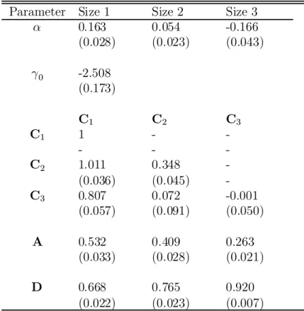
Table 4 reports the results of estimating (23) using Gaussian Q-MLE techniques. We observe some substantial changes in point estimates of the size 1 and size 3 portfolios. The size one intercept increases from 0.108 to 0.163 while the size 3 intercept declines from -.004 to -.166, a substantial increase in absolute value. Estimates of the conditional covariance matrix appear to be consistent with typical results from estimating GARCH models. All portfolios are signi¯cantly in°uenced by both shocks to volatility (A) and memory in volatility (D). We do ¯nd that the portfolio of smaller ¯rms are more (less) in°uenced by shocks (memory) than are the portfolios of larger ¯rms. These are again consistent with stylized facts of these models.
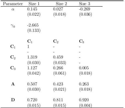
Table 5 reports the results of estimating (23) using our semiparametric estimator with the Bi-Quartic kernel (similar results were obtained with the Gaussian kernel and are not reported to save space). In computing our kernel estimate of the score we make use of Schuster's (1985) correction. See the Appendix for descriptions of the kernels and of Schus-ter's correction. We use the Box-Cox transformation with zt = ¿(wt) = wt³¡1
³ with³ = 21n in construction of the semiparametric estimates. This choice of ³ is found by HLV (2001) to yield good results in Monte Carlo experiments in a linear model. We also use separate optimal MISE bandwidth parameters (¾T) for estimating °(z) and °0(z). In estimating the conditional expectation Eb£vec¡"t"Tt
¢ jwt
¤
as given by (18), we set the number of draws M=500. Results were not sensitive to larger choices for this number.
Standard errors tend to fall somewhat when using the semiparametric e±cient estimator rather than the Gaussian Q-MLE, and the point estimates of ® using the semiparametric estimator tend to be smaller than for their Q-MLE counterparts. The Wald test statistics of the validity of the CAPM, formed from the ® estimates, are given in Table 6. For the unconditional CAPM, we ¯nd that OLS leads to a marginal rejection of the CAPM at the 5% level. When we look at the tests of the C-CAPM both estimation methods lead to strong rejections of the model with p-values less than .01.
Although the inferences regarding ® are quite similar for the two methodologies, we ¯nd some potentially interesting di®erences in the estimated systematic risk as measured by beta (¯t). These di®erences are seen in Tables 4 and 5, listing the parameter estimates, or perhaps more easily observed in Figures 1-3. These ¯gures plot the conditional betas for the
three portfolios showing the Q-MLE beta as well as the semiparametrically estimated beta using the Bi-Quartic kernel. We observe that the ¯1;t (size 1 portfolio) tends to be higher for the Q-MLE relative to the semiparametric estimates. However, for the other two size portfolios the estimated¯t is greater for the semiparametric estimator than for the Q-MLE. We also ¯nd that the variability of ¯t is greater for the Q-MLE than for the semiparametric estimates. This is true for all of the size portfolios but especially for the size 1 and 2 portfolios. For these, the standard deviation of ¯t is 48% smaller for the semiparametric estimate then for the Q-MLE estimate. On the other hand the standard deviation of¯3;t is only 2% smaller for the semiparametric estimate.
We also provide graphs of conditional expected returns for the three portfolios. These graphs are found in Figures 4 through 6. We de¯ne the conditional expected return to be:
Et¡1rt=®^ + exp (^°0)H^t!t¡1:
These graphs incorporate both the intercepts and the conditional betas and give a net e®ect on the parameters of interest for our semiparametric e±cient method relative to Q-MLE methods. In general, we ¯nd that the semiparametric e±cient method leads to estimates of conditional expected return that are greater than Q-MLE methods. These di®erences are small for the size 1 portfolio but increase as we move to the larger ¯rm portfolios. We observe that the di®erences in the estimates of the scaled conditional covariance matrix (Ht) tend to dominate di®erences in the intercept (®). In general, the semiparametric method estimates a larger portion of return due to systematic risk and a smaller portion of return coming from unexplained e®ects relative to Q-MLE.
6. SIMULATIONS
We simulated series of multivariate GARCH(1,1) time series using the following data gener-ating process,
rt=®+ exp (°0)Ht!t¡1+ut; (24)
with
Ht =CCT+Aut¡1uTt¡1A: We setn= 2; T = 759; and use the following parameterizations:
C= · 1 0 0 1:15 ¸ ;A = · :5 0 0 :25 ¸ ;
and °0= ¡2:75: This simulation set-up is a simpli¯cation of our empirical model, adopted for the purpose of reducing the computer time required to run the simulations. We use the same !t¡1 from our empirical analysis but reduce the dimension to a 2£1 vector by combining the smaller two decile weights into one. We also simulate data using two di®erent
®vectors, ®=f0;0g under the null and®=f¡:15; :15gunder the alternative.
We add a randomly selected residual (ut) from some prespeci¯ed distribution. We consider a normal, a mixture of normals, a Student-t with 3 degrees of freedom, and Chi-Square with 5 degrees of freedom. The ¯rst three distributions are elliptical, while the third is asymmetric and is included as a check on the robustness of our estimator to misspeci¯cation. To compute the mixture of normals, we ¯rst de¯ne the uniform random variableU 2[0;1]:
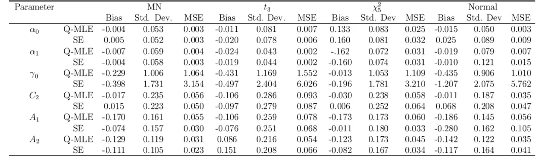
If U < (1¡²), then let ut = p·1u¸t, where u¸t sN(0;1). Otherwise, we let ut =p·2¸ut, . The resulting ut will follow a mixed normal distribution. We set²= :8; ·1 = 0:65 in the simulations, and for all distributions the errors are scaled to have unit variances. We use the same residual in constructing both the alternative and null series. For each simulation we estimate (24) using Q-MLE and the semiparametric e±cient estimator. We replicate each simulation 2,000 times for each distribution and report the results of the simulations in Tables 7 - 9.
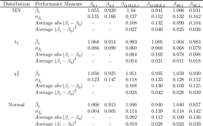
Table 7 reports bias, standard deviation, and mean squared error (MSE) for the estima-tors for the four di®erent distributions. For the nonnormal elliptical densities, the semi-parametric estimator (SE) yields only slight improvements in estimation of the intercepts, with larger improvements found in the estimation of the conditional variance parameters. This is consistent with our empirical study, where we found that the SE point estimates had greater impact on conditional covariances than on intercepts. Estimation of the risk aversion parameter °0 deteriorates when we move from the Q-MLE to the SE, but neither estimator accurately estimates this parameter. We should point out that for the purposes of the present paper, °0 is not of substantive interest, as we have focused our attention on testing for zero interecepts and estimating betas, for both of which problems °0 can be thought of as a nuisance parameter. Note that in the case of asymmetric errors, the SE provides reasonably good estimates of most of the parameters. This is important because, recalling our earlier comments, we have no theoretical results on the behaviour of the SE under asymmetry, but the simulation results suggest that the SE may be robust to asymme-try. For the case of normal errors we see deterioration in the SE estimation of conditional mean parameters, where MSE are at least twice as large as their MLE counterparts. The SE estimates of conditional variance parameters are much closer to their MLE counterparts. Table 8 compares the simulation results in estimation of beta. For each simulation, we use the true parameter values and the simulated residuals to construct a time series of `true' betas¡¯i0¢, where i indexes the simulation. We compute the average values of ¯i0 for each portfolio over the time series as well as the standard deviations of ¯i0, ³¾¯i
0;j
´
for each simulation. We then de¯ne ¯0;j = 20001
P2000 i=1 ¯ i 0;j, and ¾¯0;j = 1 2000 P2000 i=1 ¾¯i 0;j for j = 1;2. We construct this same measure using the parameter and residual estimates from the two estimation methods. The ¯nal two measures reported in Table 8 are constructed by looking at absolute and squared di®erences between the estimated and `true' conditional betas for each simulation and then averaging over the simulations. One apparent advantage of the semiparametric estimator is that estimated volatilities of the conditional betas are closer to the `true' beta volatilities than for the Q-MLE estimates. Note that in our empirical application, the SE produces less volatile estimated betas than the Q-MLE, while the reverse is true in the simulations. We are not sure why this is the case, althought the simulation set-up is di®erent in a couple of important ways from the empirical model, which may explain the di®erence in results. The important point to take note of, in our view, is that the SE betas have a volatility that is closer to the true beta volatility than the Q-MLE betas. We also note that the performance of the SE estimated betas for the simulation with normal residuals indicates that there is a loss relative to the MLE estimator. However, the losses for this case are approximately of the same order as the gains in the nonnormal simulations and
given the prevalence of nonnormality in the data, the performance of the SE beta estimates are remarkably good.
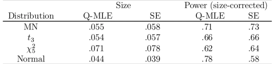
Table 9 considers the Wald tests of the zero-intercept null hypothesis. We calculate the empirical size and power of the test statistics for the two estimation methods as discussed in Davidson and MacKinnon (1998) using the p-values from each test statistic. The power results are adjusted for any biases in size. The two methods lead to quite similar size and power properties in the asset pricing tests for all of the cases other than normality; the SE being slightly more over-sized but having slightly higher size-corrected power. Both methods lead to reasonably sized tests for the elliptical distributions but over-reject for the asymmetricÂ2
5distribution. The MLE method has substantially greater power than the SE method for the case of normality.
7. CONCLUSION
We propose a new estimation methodology that captures the nonnormalities of return dis-tributions arising from tail thickness by employing a multivariate GARCH-in-mean model with the °exible distributional assumption of conditional elliptical symmetry. Under high level assumptions, this framework should lead to more e±cient estimates than quasi-MLE and should yield more powerful asset pricing tests. We ¯nd in empirical and simulation analysis that our estimator does not improve signi¯cantly over the Gaussian Q-MLE in the estimation of conditional mean parameters, but that the semiparametric e±cient estimates of the conditional betas do improve on the Q-MLE estimates to a degree that may be of potential interest to applied workers.
Further work on the properties of our estimator in the presence of speci¯cation failure is suggested. In particular, the work of Harvey and Siddique (1999), among others, suggests that a derivation of the semiparametric e±ciency bounds of the GARCH-in-mean model with conditional densities that are not required to be symmetric would be a useful contribution to this research. We have seen in our simulations that the estimator in this paper does not misbehave too badly in the presence of asymmetric errors, but it would be desirable to have an estimator that explicitly accounts for the possibility of asymmetry. Such an estimator would have to take account of the fact that the conditional location is unidenti¯ed in the presence of asymmetric errors of unknown distributional form, and would require the use of multivariate generalizations of the approaches taken by Newey and Steigerwald (1997) and Drost and Klaassen (1997), both of which studies analyze univariate GARCH models with possibly asymmetric conditional densities of unknown functional form.
8. APPENDIX
8.1. Elliptical Densities1. An n-dimensional random vector u is said to be elliptically distributed about the origin if its density can be written as
p(u) = (det §)¡1=2g¡u0§¡1u¢;
where § is a positive de¯nite, symmetric matrix that is proportional to the covariance matrix of u (when a ¯nite covariance matrix exists) and is also proportional to the inverse of the
information matrix of p. The characteristic function of u is Ã(s) =E£exp¡isTu¢¤=Á¡sT§s¢
for some function Á(¢): The standardized n-vector " = §¡1=2u is said to be spherically symmetric, with density
p(") = g¡"T"¢:
Note that the isoprobability contours of the density of the elliptical random variable u will be elliptical in shape, and those of the spherical random variable " will be spherical (circular in the case of n= 2).
Some examples of spherical densities are: (a) the Gaussian,
g(¢) =const¢exp µ ¡" T" 2 ¶ ; (b) the Student'st with¿ degrees of freedom,
g(¢) =const¢ µ 1 + " T" ¿ ¶¡(n+¿)=2 ; (c) the Cauchy, g(¢) =const¢¡1 +"T"¢¡(n+1)=2; (d) the logistic,
g(¢) =const¢exp¡¡"T"¢=£1 + exp¡¡"T"¢¤2; (e) and the scale mixed normal,
g(¢) =const¢ Z 1 0 s¡n=2exp µ ¡" T" 2s ¶ dF (s)
for some cdf F(¢): Note that all the non-Gaussian densities listed here feature thick tails and some of them are popular candidates for modeling tail thickness in empirical work that takes a fully parametric tack.
Elliptical distributions have a few properties that are of interest. First, de¯ne the norm
k"k = p"T": The random variables "
k"k and k"k are independent of one another. Further-more, the random variable k""k has a uniform distribution on the (n¡1)-dimensional unit hypersphere. These two features of elliptical distributions form the basis for Beran's (1979) test for elliptical symmetry, while the latter fact plays a central role in our derivation of the semiparametric e±ciency bound for this model, following the results of Brown and Hodgson (2000).
De¯ne the n¤£n matrix ©, of rank n¤ ·n: Then the n¤-dimensional random variable ©u is elliptically symmetrically distributed with characteristic matrix of ©§©T: De¯ne the partition u=¡uT
1; uT2
¢T
and partition § conformably as
·
§11 §12 §21 §22
¸ :
Then the marginal densities ofu1and u2are of the same form as the joint density of u, with respective characteristic matrices of §11 and §22: The conditional mean can be written as
E[uijuj] = §ij§¡jj1uj:
Furthermore, the density of ui conditional on uj will be elliptically symmetric with a char-acteristic matrix of §ii ¡§ij§¡jj1§ji:
Many of these characteristics of elliptical distributions are well known among economists to apply to the Gaussian density. That they also apply to the more general elliptical family explains why the unconditional CAPM also holds in this case, a point which is discussed in more detail by Owen and Rabinovitch (1983).
8.2. Computation of Derivatives. We remark here on the di±culty of obtaining ex-pressions for the derivatives @lnjHtj
@µ , @uT
t
@µ and
@(vecH¡t1)T
@µ . The basic problem is that each of these derivatives involves an in¯nite recursion, since the expression for @uTt
@µ , for example, in-volves @(H@µt)T, which in turn involves @uTt¡1
@µ , and so on. Our practical approach is to construct the derivatives by assuming that @vec(H0)
@µ and @u0
@µ take on their unconditional values which allow us to obtain @vec@µ(H1) and @@µu1. Given the derivatives for period one we can construct the same for period two and continue in a likewise manner to construct the derivatives for all T periods. We could also have assumed that @vec(H0)
@µ and @u0
@µ are zero, following Drost and Klaassen (1997), but have found in preliminary calculations that the empirical properties of the estimator were quite robust to the assumptions placed on @vec(H0)
@µ and @u0
@µ. As stated earlier, the asymptotics of the estimator should not depend upon the assumptions of the initial period.
8.3. Kernels and Trimming. The two kernels we consider are the bi-quartic, K¾(u) = 15 16 µ 1¡ u 2 ¾2 ¶2 In¯¯¯u¾¯¯¯ ·1o; and the Gaussian
K¾(z) = 1 ¾p2¼ exp µ ¡ z 2 2¾2 ¶ :
The bi-quartic is applied without trimming. To establish consistency of the Gaussian kernel estimator, it is su±cient to apply the following trimming conditions, as shown by HLV (2001): (i) b°t(z)¸dT; (ii) jzj · eT; (iii) j¸(z)j ·bT; (iv) ¯¯½1=2(z)b°0 t(z)¯¯·cTb°t(z); where½(z) =w¿0(w)J¡1 ¿ (w) (recall thatw=¿¡1(z)),J¿(z) = ¯ ¯¯@¿¡1(z) @z ¯ ¯¯, and (d=dz)¡1½1=2(z): The constants ¾T, dT; eT; bT;andcT have the properties that, as T ! 1, we have¾T ! 0; cT ! 1; eT ! 1; bT ! 1; dT ! 0, ¾TcT !0; eT¾T¡3=o(T), and bT¾T¡3 =o(T):
8.4. Schuster's Correction. For most standard choices of symmetric kernel, the den-sity estimatorfT(z) typically performs poorly on the right neighborhood of zero. This bias arise because for points xi in the right neighborhood of 0, the contribution of xi given by T¡1K¾T(x¡xi)to fT(x) extends to points x·0 where f(x) = 0:A similar bias arise in the multivariate density estimates which impose the elliptical symmetry restriction. This bias creates a volcano like contour in the density estimate. The over°ow in weights beyond the lower support of 0 can be corrected by using an estimator which incorporates this additional support constraint information into fT(x).
Schuster (1985) o®ers a correction that incorporates this over°ow to the region z < c, for ¯nite c, back into the region z ¸ cby adding a mirror image term T¡1K
¾T(z ¡2c+zs) to
T¡1K¾T(z¡zs):The resulting estimator forz ¸c is given by
b °t(z) = (T ¡1)¡1 T X s=1 s6=t [K¾T(z¡zs) +K¾T(z¡2c+zs)]:
In our case, c= 0:Schuster (1985) also proves consistency and asymptotic normality results for this estimator.
References
[1] Beran, R., 1979, Testing for ellipsoidal symmetry of a multivariate density, Annals of Statistics, 7:150-162.
[2] Berk, J., 1997, Necessary conditions for the CAPM, Journal of Economic Theory 73, 245-257.
[3] Bickel, P. J., 1982, On adaptive estimation,Annals of Statistics 10, 647-671.
[4] Black, F., M. Jensen, and M. Scholes, 1972, The capital asset pricing model: some empirical tests, in Jensen, M. (ed), Studies in the Theory of Capital Markets, New York, Praeger.
[5] Bollerslev, T., 1987, A conditional heteroskedastic time series model for speculative prices and rates of return, Review of Economics and Statistics 69, 542-547.
[6] Bollerslev, T., R. Chou, and K. Kroner, 1992, ARCH modelling in ¯nance: A review of the theory and empirical evidence,Journal of Econometrics 52, 5-59.
[7] Bollerslev, T., R. Engle, and J. Wooldridge, 1988, A capital asset pricing model with time varying covariances,Journal of Political Economy 96, 116-131.
[8] Bollerslev, T. and J. Wooldridge, 1992, Quasi-maximum likelihood estimation and in-ference in dynamic models with time-varying covariances, Econometric Reviews 11, 143-172.
[9] Box, G. and D. Cox, 1964, An analysis of transformations, Journal of the Royal Statis-tical Society, Series B, 211-264.
[10] Box, G. P., and D. A. Pierce, 1970, Distribution of residual autocorrelations in au-toregressive integrated moving average time series models, Journal of the American Statistical Association, 65, 1509-1526.
[11] Braun, P.A., Nelson, D.B. and Sunier, A.M. 1995. Good news, bad news, volatility, and betas. Journal of Finance 50:1575-1603.
[12] Brown, B.W. and D. Hodgson, 2000, E±cient semiparametric estimation of dynamic nonlinear systems under elliptical symmetry, Unpublished manuscript.
[13] Buse, A., B. Korkie, and H. Turtle, 1994, Tests of conditional asset pricing with time-varying moments and risk prices, Journal of Financial and Quantitative Analysis, 29, 15-29.
[14] Campbell, J., W. Lo, and A. C. MacKinlay, 1997,The Econometrics of Financial Mar-kets, Princeton, Princeton University Press.
[15] Chamberlain, G., 1983, A characterization of the distributions that imply mean-variance utility functions, Journal of Economic Theory 29, 185-201.
[16] Davidson, R., and J., MacKinnon, 1998, Graphical methods for investigating the size and power of hypothesis tests, The Manchester School 66, 1-26.
[17] De Santis, G., and B. Gerard, 1998, International asset pricing and portfolio diversi¯-cation with time-varying risk, Journal of Finance, forthcoming.
[18] Diebold, F., 1988, Empirical Modeling of Exchange Rate Dynamics,New York, Springer-Verlag.
[19] Drost, F. and C. Klaassen, 1997, E±cient estimation in semiparametric GARCH models,
Journal of Econometrics, 81, 193-221.
[20] Engle, R., 1982, Autoregressive conditional heteroskedasticity with estimates of the variance of UK in°ation, Econometrica, 50, 987-1008.
[21] Engle, R., and K. Kroner, 1995, Multivariate simultaneous generalized ARCH, Econo-metric Theory 11, 122-150.
[22] Fama, E., 1965, The behavior of stock market prices, Journal of Business 38, 34-105. [23] Fama, E. and J. MacBeth, 1973, Risk, return and equilibrium: Empirical tests, Journal
of Political Economy 81, 607-636.
[24] Fang, K., S. Kotz, and K. Ng, 1990, Symmetric Multivariate and Related Distributions,
London, Chapman and Hall.
[25] Gibbons, M., 1982, Multivariate tests of ¯nancial models: A new approach. Journal of Financial Economics 10, 3-27.
[26] Harvey, C., 1989, Time-varying conditional covariances in tests of asset pricing models,
Journal of Financial Economics 24, 289-317.
[27] Harvey, C., 1991, The world price of covariance risk,Journal of Finance 46, 111-157. [28] Harvey, C. and A. Siddique, 1999, Autoregressive conditional skewness, Journal of
Fi-nancial and Quantitative Analysis, 34:465-487.
[29] Hodgson, D.J., 1998, Adaptive estimation of cointegrating regressions with ARMA er-rors, Journal of Econometrics, 85:231-267.
[30] Hodgson, D., O. Linton, and K. Vorkink, 2001, Testing the capital asset pricing model e±ciently under elliptical symmetry: a semiparametric approach. In press, Journal of Applied Econometrics.
[31] Jagannathan, R., and Z. Wang, 1996, The conditional CAPM and the cross-section of expected returns,Journal of Finance 51, 3-53.
[32] Jarque, C. and A. Bera, 1980, E±cient tests for normality, heteroskedasticity, and serial independence of regression residuals,Economics Letters 6, 255-259.
[33] Jeantheau, T. 1998. Strong consistency of estimators for multivariate ARCH models.
Econometric Theory 14:70-86.
[34] Linton, O., 1993, Adaptive estimation in ARCH models, Econometric Theory, 9, 539-569.
[35] Linton, O.B. and D.G. Steigerwald, 2000, Adaptive testing in ARCH models, Econo-metric Reviews, 19, 145-174.
[36] MacKinlay, A. C., and M. Richardson, 1991, Using generalized method of moments to test mean-variance e±ciency, Journal of Finance 46, 511-527.
[37] Mandelbrot, B., 1963, The variation of certain speculative prices, Journal of Business
36, 394-419.
[38] Mardia, K.V., 1970, Measures of multivariate skewness and kurtosis with applications,
Biometrika 57, 519-530.
[39] Merton, R., 1973, An intertemporal capital asset pricing model, Econometrica 41, 867-887.
[40] Mitchell, A., 1989, The information matrix, skewness tensor, and ®-connections for the general multivariate elliptic distribution, Annals of the Institute of Mathematical Statistics, Tokyo, 41, 289-304.
[41] Muirhead, R., 1982, Aspects of Multivariate Statistical Theory,New York, Wiley. [42] Nelson, D., 1991, Conditional heteroskedasticity in asset returns: A new approach,
Econometrica 59, 347-370.
[43] Newey, W.K., 1990, Semiparametric e±ciency bounds, Journal of Applied Economet-rics,5:99-135.
[44] Newey, W.K. and D.G. Steigerwald, 1997, Asymptotic bias for quasi-maximum-likelihood estimators in conditional heteroskedasticity models, Econometrica, 65:587-599.
[45] Owen, J., and R. Rabinovitch, 1983, On the class of elliptical distributions and their applications to the theory of portfolio choice, Journal of Finance 38, 745-752.
[46] Schuster, E., 1985, Incorporating support constraints into nonparametric estimators of densities. Communications in Statistics - Theory and Methods 14, 1123-1136.
[47] Schwert, G., and P. Seguin, 1990, Heteroskedasticity in stock returns,Journal of Finance
45, 1129-1155.
[48] Stambaugh, R., 1982, On the exclusion of assets from tests of the two-parameter model: A sensitivity analysis.Journal of Financial Economics 10, 237-268.
[49] Vorkink, K., 2001, Return distributions and improved tests of the capital asset pricing model, Working paper, Brigham Young University.
[50] White, H., 1982, Maximum likelihood estimation of misspeci¯ed models, Econometrica
50:1-25.
[51] Zhou, G., 1993, Asset pricing tests under alternative distributions, Journal of Finance
Table 1. Summary Statistics
Portfolios Mean Std. Dev. min max Kurtosis J-B
Size 1 0.276 1.870 -19.377 8.510 73.313¤ 11513¤
Size 2 0.255 2.231 -21.590 9.548 46.721¤ 6747¤
Size 3 0.332 2.799 -24.301 15.453 45.721¤ 2890¤
Note: This table provides statistical characteristics of the portfolios of excess returns used in our in our empirical analysis. The stock returns are obtained from the CRSP data set. The series are daily returns from Jan. 1995 through Dec. 1997. Estimates of kurtosis have been scaled so that under the assumption of normality the statistics have an asymptotic N(0,1) distribution.
J-B refers to the Jarque-Bera (1980) test for normality. ¤Refers to a rejection of the
hypothesis that the given moment is consistent with the Normal distribution at the .01 level.
Table 2. Multivariate Tests of Conditional Normality and Elliptical Symmetry Panel A: Multivariate Kurtosis Test
Size Portfolios
Unconditional Returns 17.054¤
Unconditional Residuals 17.726¤
Conditional Returns 4.395¤
Conditional Residuals 6.167¤
Panel B: Elliptical Symmetric Test (Sn)
Size Portfolios
Conditional Returns 1.5991
Conditional Residuals 0.4261
Note: The test statistics below are Mardia's (1970) multivariate kurtosis measure and Beran's (1979) test for elliptical symmetry. Tests are constructed using the series of
portfolio returns (rt)and residuals (ut) and where both series are weighted by the matrix
Ht1=2. The multivariate kurtosis measure has been scaled so that assuming normality the
statistic will have an asymptotic N(0,1) distribution. ¤Indicates a p-value less than .01.
Table 3. OLS Estimation of the Unconditional CAPM
® ¯im
Portfolio Estimate Std. Error Estimate Std. Error
Size 1 0.108 0.050 0.475 0.018
Size 2 0.032 0.049 0.659 0.018
Size 3 -0.004 0.004 1.031 0.001
Note: Data are from the CRSP data set of stocks listed on the NYSE, AMEX, and NASDAQ. Value-weighted returns are calculated daily from January 1996 through December 1997. Three size portfolios are created according to the previous day's market value of equity. The previous day's NYSE size quartiles are used as the cuto®s for the size portfolios. The CAPM model takes on the
following parameterization: rt =®+¯rm;t+ut: Above are results from