Control and synchronization of the generalized Lorenz system with mismatched uncertainties using backstepping technique and time‐delay estimation

Control and Synchronization of the Generalized Lorenz System with Mismatched

Uncertainties using Backstepping Technique and Time-delay Estimation

Dongwon Kim1, Maolin Jin2 and Pyung Hun Chang3*

1

Department of Mechanical Engineering, University of Michigan, Ann Arbor MI 48109

2_{Korea Institute of Robot and Convergence (KIRO), Pohang, Korea}

3_{Department of Robotics Engineering, Daegu-Gyeongbuk Institute of Science and Technology (DGIST), Daegu} 711-873,

Korea

*Correspondence: [email protected], +82.53.785.6260

Abstract

We propose a robust control technique for regulation and synchronization of the Generalized

Lorenz System (GLS) that covers the Lorenz system, Chen system and Lü system. The

proposed control provides synergy through the combination of the backstepping control and

time-delay estimation

(TDE) technique. TDE is used to estimate and cancel nonlinearities and

uncertainties, and the backstepping method is adopted to provide robustness against matched

and mismatched uncertainties. As a result, we observe in numerical simulation that the

proposed technique shows better performances in regulating and synchronizing the GLS with

mismatched uncertainties, in comparison with existing schemes. The efficacy of the proposed

technique is also validated with a circuit-implemented chaotic system.

Keywords: Chaotic system; Robust control; Synchronization; Chaotic circuit; Time-delay

estimation; Backstepping.

1. Introduction

Chaotic behaviors provide various applications based on their irregularity and unpredictability. These applications are shown in various fields, including physical, chemical and ecological systems, secure communications [1, 2, 45]. A variety of control theories have been applied to manage chaotic signals [3–12, 30–36]. Recently, for a faster response and enhanced robustness, hybrid methods have appeared in regulating and synchronizing chaotic systems. For example, adaptive control and backstepping technique are combined in [8, 13, 14], optimal control and sliding mode control are used together in [11], fuzzy logic, adaptive control and sliding mode control are merged in [9, 12, 15, 33]. These approaches, however, require a precise chaotic system model, and are vulnerable to parameter variations, modeling errors and external disturbances. Moreover, the hybrid methods are quite complicated.

simplicity and robustness [17]. Jin and Chang’s technique comprises three parts: a TDE part to cancel the controlled system’s dynamics, an injection part to endow the desired master system’s dynamics, and a convergence part to shape the synchronization error dynamics. It provides fast, accurate and robust performance. With the TDE technique, Kim et al. also proposed a regulation and synchronization method using terminal sliding mode (TSM) [18]. Kim’s method achieves fast and powerful convergence. The aforementioned two methods based on the TDE technique [17], [18] have no device for suppressing mismatched uncertainties; they are vulnerable to uncertainties that do not satisfy the matching condition.

Suppressing the effect of mismatched uncertainties is important in minimizing the number of control inputs and sensors. In this paper, we propose a simple robust technique that is able to care of mismatched uncertainties in a chaotic system as well as matched uncertainties, through the combination of combine the backstepping technique and TDE technique. The backstepping method enables a systematic and recursive procedure for the design of control laws for systems in strict feedback form, while TDE enables a simple effective compensation for uncertainties. Therefore, the proposed technique provides a single controller that can be applied to any systems in strict feedback form even if a precise system model is not identified. In addition of this benefit, uncertainties that reside on each equation of chaotic systems can be suppressed by TDE conducted on the equation, and all TDE on each equation are governed by the control input. The proposed technique is therefore expected to be superior in dealing with mismatched uncertainties.

To verify the efficacy of the proposed technique, we apply the technique to the regulation and synchronization problems of the Generalized Lorenz System (GLS) introduced in [21, 22]. The GLS covers the well-known classical Lorenz system [23], Chen system [24] and Lü system [25] in one formulation. We perform a comparative study with the TDE-based controllers proposed in previous works [17, 18]. The proposed technique is experimentally validated with a circuit-implemented chaotic system.

This paper is an extension of our previous work originally reported in our short proceeding [1]. In this paper, we additionally provide the stability analysis for the closed-loop system with the proposed technique, and present a real experimental data. Experimental implementation is crucial for practical applications of chaos [11, 26–29] because the signal is always contaminated by noise. Numerical differentiation of state variable is required to implement the proposed technique, and it can easily amplify the noise effect; thus, the proposed technique should be verified through experiment or, at least, computer simulation considering noise. In this paper, we will verify the proposed control through physical chaotic systems with analog circuit elements.

This paper begins with the design procedures of controllers each of which is tailored to the regulation and synchronization problems, respectively, with a brief explanation of the GLS. In the following sections, the proposed controllers are validated through a simulation study and experimental study. We allocate subsections separately to the regulation and synchronization parts as well in these validation studies. Finally, we make remarks in the conclusion section.

2. Controller development 2.1 Regulation

The Generalized Lorenz System (GLS) [2] is described as 11 12 1 3 21 22 0 0 0 0 0 0 1 , , 0 0 1 0 a a x a a

λ

    _{ }   =_{ } + _ − _ =_{ }     _{ }   A x x x A (1)

where x=

[

x₁ x₂ x₃

]

T,

λ

₃

∈

R



,

and matrix

A

has eigenvalues

λ λ

₁, ₂∈R,

λ

_2,3<0,

λ

₁ >0. The control objective is to regulate x to a specific constant

2 1 1 1 3

[

d

]

T d d d

x

x

x

λ

=

−

x

. If

x t

₁

( )

converges to a specific point

x

_1d, state x t₂( ) converges to the specific point

x

_1d as well from the fact that x t₁( )=0. Once x t₁( ) and x t₂( ) converge to specific a point

x

_1d, state x t₃( ) converges to a certain point based on the characteristic that the parameter (eigenvalue)λ₃<0 (Eq. (1)). Considering this fact, we can separate the GLS into two parts as follows:

1 11 1 12 2 1 2 21 1 22 2 1 3 2 3 3 3 1 2

,

First part:

,

Second part:

,

x

a x

a x

d

x

a x

a x

x x

d

x

λ

x

x x

=

+

+



 =

+

−

+



=

+







(2)

where

d

₁ and

d

₂ denote unknown disturbances, which are assumed to be continuous and bounded.

Now, it is required to control the first part of the generalized Lorenz system to achieve the control objective. The control of the first part can be achieved by adding a control input u to the differential equation of state

x

₂. In order to design a robust backstepping technique, we transform the first part of Eqs. (2) as follows: 1 11 1 12 2 1 1 1 1 2 1 1 1 2 2 21 1 22 2 1 3 2 2 2 2 2 2 2

ˆ

,

,

,

ˆ

,

,

,

x

a x

a x

d

x

f

g x

x

h

g x

x

a x

a x

x x

d

u

x

f

g u

x

h

g u

=

+

+

= +

= +







⇒

⇒



=

+

−

+

+



=

+



= +



















(3) where 1 11 1 1 1 12 2 21 1 22 2 1 3 2 2

,

,

,

1,

f

a x

d

g

a

f

a x

a x

x x

d

g

=

+

=

=

+

−

+

=

(4)

and h i_i( =1, 2) are terms that include all uncertainties:

1 11 1 12 1 2 1 2 21 1 22 2 1 3 2 2

ˆ

(

)

,

ˆ

(1

) ,

h

a x

a

g x

d

h

a x

a x

x x

d

g u

=

+

−

+

=

+

−

+

+ −

(5)

where

g

ˆ

₁ and

g

ˆ

₂ are constants.

With a definition e₁  x_1d −x₁, a Lyapunov function

V

₁ can be designed as 2 1 1

1

.

2

V



e

(6)

The time derivative of

V

₁ is

1 1 1 1( 1d 1 ˆ1 2).

V =e e =e x − −h g x (7)

From Eq. (7), treating

x

₂ as a virtual control effort, the ‘desired control effort value

x

_2d’ for

x

₂ is chosen so that the negative definiteness of V₁ is guaranteed.

2 1 1 1 1 2 1 1 1 1 1

,

ˆ

(

),

d d

V

C e

x

g

−

x

h

C e

= −

+ +







(8)

where

C

₁ is a design parameter.

Since x_2d =gˆ (₁−1 x_1d − +h₁ C e_{1 1}) is a desired control effort and differs from the real state

x

₂, we denote this ‘desired control effort value’ as

x

_2d. It is then necessary to find a way to realize

x

_2d. The next step of the backstepping design is to make the error between

x

₂ and

x

_2d as small as possible.

The actual control effort u is designed so that the error between

x

₂ and

x

_2d converges to zero. The error between

x

₂ and

x

_2d is defined as follows:

2 ˆ (1 2d 2)

e g x −x . (9)

We define a Lyapunov function candidate

V

₂ as

2

2 2

1

2

V



e

. (10)

2

2 2 2 2

ˆ

1

(

2d 2

)

2

(

1d 1 1 1

ˆ

1 2

ˆ ˆ

1 2

)

2 2

V



=

e e



=

e g x



−

x



=

e x



− +

h



C e



−

g h

−

g g u

= −

C e

. (11) From Eq. (11), the actual control effort u is chosen so that the negative definiteness of V₂ is guaranteed. 1 1 2 1 1 2 1 1 1 2 2

ˆ ˆ

ˆ

(

) (

_d

),

u

=

g g

−



x

+

g h

+ +

h



C e



+

C e

(12)

where

C

₂ is a design parameter.

Now, we need to estimate the value of the term g hˆ_{1 2}+h₁. Differentiating the first equation of Eqs. (3) with respect to time gives

x



₁

= +

h



₁

g h

ˆ

_{1 2}

+

g g u

ˆ ˆ

_{1 2}

=

H

+

Bu

,

(13) where Hg hˆ_{1 2}+h B₁, g gˆ ˆ_{1 2}. With the assumption that

d

₁ and

d

₂ are continuous, it is reasonable to regard H as a continuous function. It is obvious that the states of GLS are continuous (see Eq. (1)). Then, we could build an approximation H t( )≅H t( −L), provided that the sampling period L is sufficiently small. This estimation, called TDE [37–44], is formally defined as

ˆ ( )

(

).

H t

=

H t

−

L

(14)

For a practical use, the estimate of the term H can be obtained as, using Eq. (13),

H t

ˆ ( )

=

H t

(

−

L

)

=



x t

₁

(

−

L

)

−

B u t

−1

(

−

L

).

(15) TDE is obtained by using the previous-step sensor reading and record of the previous-step input. If the time delay L is sufficiently small, the TDE can estimate and cancel out the system nonlinearities and uncertainties of the system dynamics [37–44]. Therefore, the TDE technique provides simplicity and robustness against uncertainties without substantial computation load. Substituting Eq. (15) into Eq. (12), with the relationship

e

₂

= +

e



₁

C e

_{1 1}, leads to the final form of the actual control input as follows:

1

1 1 1 2 1 1 2 1

( ) ( _d ( ) ( ) ).

u=u t−L +B− x −x t−L + C +C e +C C e (16) The control gains

C

₁ and

C

₂ determine how fast the error

e

₁ converges. In Eq. (16), the

delayed acceleration is calculated by numerical differentiation [37–44], as

(

)

2

1( ) 1( ) 2 (1 ) 1( ) /

x t−L = x t − x t− +L x t L

2.2 Stability Analysis

The stability analysis of the overall closed-loop system is performed and the sufficient condition for closed-loop stability is derived. If the exact value of H was able to be identified, the closed-loop system with the control input would be asymptotically stable, based on the Lyapunov stability theorem. However, since the value of H is estimated using TDE, stability is not guaranteed due to the difference between the real value of H and its estimate. Here, we analyze the stability of the closed-loop system taking the difference into account, grounded on the proof presented in [19].

-1

( )t

[

( )t

-

( )t

],

u

=

B v

H



(17)

where

v

_{( )t}





x

_{1 ( )d t}

+

(

C

₁

+

C e

₂

)



_{1( )t}

+

C C e

_{1 2 1( )t}

.

Differentiating the first equation of (3) with respect to time gives

x



_{1( )t}

=

H

_{( )t}

+

Bu

_{( )t}

.

(18) Substituting Eq. (17) into Eq. (18) yields

x



_{1( )t}

-

v

_{( )t}

=

H

_{( )t}

-

H



_{( )t}

.

(19) With TDE error ε(t) defined as

( )t

v

( )t

-

x

1( )t

H

( )t

-

H

( )t

,

ε





=



(20)

we obtain the error dynamics of the proposed control:

e



_{1( )t}

+

(

C

₁

+

C e

₂

)



_{1( )t}

+

C C e

_{1 2 1( )t}

=

ε

_{( )t}

.

(21) From the error dynamics, the tracking error e1(t) is influenced by TDE error ε(t). If ε(t) is asymptotically

bounded, then the error dynamics is also asymptotically bounded [19], and consequently the overall closed-loop system is stable. Therefore, we focus on the boundedness of ε(t) from now on. To this end,

a differential equation representing thedynamics of ε(t) is derived.

1( )t

x



in Eq. (3) can be arranged as follows:



x

_{1( )t}

=

a

_{( )t}

+

B u

_{( ) ( )t t}

,

(22)

( )t 1( )t 1( )t 2( )t 1( )t 2( )t

.

a

=

f



+

g



x

+

g

f

(24)

The combination of Eq. (18) with Eq. (22) gives

H

_{( )t}

=

a

_{( )t}

+

[

B

_{( )t}

−

B u

]

_{( )t}

.

(25)

Using Eq. (20), we can arrange Eq. (25) as follows:

ε

_{( )t}

=

H

_{(t L}− ₎

-

H

_{( )t}

=

a

_{(t L}− ₎

+

[

B

_{(t L}− ₎

- ]

B u

_{(t L}− ₎

- (

a

_{( )t}

+

[

B

_{( )t}

- ]

B u

_{( )t}

).

(26)

Substituting Eqs. (15) and (19) into Eq. (26) gives

ε

_{( )t}

=

a

_{(t L− )}

-

a

_{( )t}

+

[

B

_{(t L− )}

- ]

B u

_{(t L− )}

-[

B

_{( )t}

- ][

B u

_{(t L− )}

+

B

−1

(-



x

_{1(t L− )}

+

v

_{( )t}

)].

(27) From the above equations, we derive the following relationships:

u

_{(t L− )}

=

B

-1

[



x

_{(t L− )}

-

a

_{( )t}

],

(28) and



x

_{1(t L}− ₎

=

a

_{(t L}− ₎

-

ε

_{(t L}− ₎

.

(29)

Finally, substituting Eqs. (28) and (29) into Eq. (27) and rearranging it give

ε

_{( )t}

=

[ -

I B B

_{( )t} -1

]

ε

_{(t L− )}

+

η

_{1(t L− )}

+

[ -

I B B

_{( )t} -1

]

η

_{2(t L− )}

,

(30)

where

η

_{1(t L− )}

=

[ -

I B B

_{( )t (}−_{t L}1_{− )}

][

x

₍( )_{t L}n_{− )}

-

a

_{( )t}

]

+

a

_{(t L− )}

-

a

_{( )t}

,

(31)

η

_{2(t L− )} =v_{( )t} -v_{(t L− )}. (32)

Taking the same approach presented in [19], the dynamics of ε(t) in Eq. (30) can be closely approximated by the dynamics behavior of the following sampled-data system (typically, control is carried out in the digital environment):

ε

_{( )k}

=

[ -

I B B

_{( )k} -1

]

ε

_(k−1)

+

η

_1(k−1)

+

[ -

I B B

_{( )k} -1

]

η

_2(k−1)

.

(33) Eq. (33) is a first order time-varying difference equation in which

η

_1(k−1)and

η

_2(k−1), from the viewpoint of ε(k), are viewed as external inputs acting as disturbances. Next, we establish a sufficient condition for the convergence of ε(k)based on Eq. (33). We assume that the convergence of ε(k) implies the convergence of ε(t)[3]. We further assume that

η

₁ and

η

₂ are bounded, and if the eigenvalues

of

I B B

-

_{( )k} -1 in Eq. (33), denoted by ξ(k), satisfy the condition that -1 < ξ(k) < 1, then ε(k)

asymptotically converges to 0. For real systems, B(g g _{1 2}) is dependent on target system parameters 1, 2

g g that are difficult and time-consuming to estimate exactly. In practice,

B

-1can be tuned without knowledge of the target system. We would recommend starting with a large positive initial value of

to tune the system performance.

2.3 Synchronization

Synchronization between two chaotic systems is achieved when each state of a slave chaotic system follows its corresponding state of a master chaotic system. Now, we apply the control technique to synchronization between two identical chaotic systems with the different initial values using one control input.

The master generalized Lorenz system and slave generalized Lorenz system are given as, respectively,

1 11 1 12 2 2 21 1 22 2 1 3 3 3 3 1 2

,

,

,

m m m m m m m m m m m m

x

a x

a x

x

a x

a x

x x

x

λ

x

x x

=

+

=

+

−

=

+







(34) 1 11 1 12 2 2 21 1 22 2 1 3 3 3 3 1 2

,

,

,

s s s s s s s s s s s s

x

a x

a x

x

a x

a x

x x

x

λ

x

x x

=

+

=

+

−

=

+







(35) where 3 1 2 3 ( , , )T m= xm xm xm ∈R

x denotes the state variables of the master system, and

3 1 2 3

( , , )T

s = xs xs xs ∈R

x denotes the state variables of the slave system.

With the state errors between the slave system and the master system defined as

1 s1 m1, 2 s2 m2, 3 s3 m3,

e x −x e x −x e  x −x (36)

the error system can be derived as

1 11 1 12 2 2 21 1 22 2 1 3 1 3 3 1 3 3 3 1 2 1 2 2 1

,

,

.

m m m m

e

a e

a e

e

a e

a e

e e

e x

e x

e

λ

e

e e

e x

e x

=

−

=

+

−

−

−

=

+

+

+







(37)

When the error states converge to zero, synchronization between two systems is achieved. Note that the parameter (eigenvalue)λ₃ is below zero. With the fact that the differential equation of the state

3

( )

e t

converges to zero when

e t

₁

( )

and

e t

₂

( )

converge to zero, the synchronization between two

1

systems can be achieved by adding a control input to the differential equation of the state

e

₂. That is, the control input is added to the differential equation of the state

x

_s2of the slave system.

1 11 1 12 2 2 21 1 22 2 1 3 1 3 3 1 3 3 3 1 2 1 2 2 1

,

First part:

,

Second part:

.

m m m m

e

a e

a e

e

a e

a e

e e

e x

e x

u

e

λ

e

e e

e x

e x

=

−



 =

+

−

−

−

+



=

+

+

+







(38)

The proposed control can be designed for the first part of Eqs. (38) with the same procedure of regulation in Section 2. The first part can be rewritten as

1 1 1 2 2 2 2

ˆ

,

ˆ .

e

h

g e

e

h

g u

= +

= +





(39)

The first part is in the same form with Eq. (3). The control input can be derived as follows in the same way proposed in Section 2:

1

1 1 1 2 1 1 2 1

( ) ( ) ( _m ( ) ( ) ).

u t =u t−L +B− x −x t−L + C +C e +C C e (40)

We emphasize that all uncertainty factors in the first part can be dealt with by TDE as long as they are included in

h

₁and

h

₂.

3. Numerical simulation

3.1 Regulation of the Lorenz system

As an example of the generalized Lorenz system to be controlled, the Lorenz system is chosen. The Lorenz system is simple but captures various features of the generalized Lorenz system. To show the robustness of the proposed controller, we take unstructured uncertainties (i.e., disturbances) as well as structured uncertainties (i.e., parameter variations) into account. Bounded continuous disturbances are considered in the differential equations of the state x and state

y

for more practical circumstances [4]. In addition, the variations of parameters

σ

, r, and

b

are also considered. Then, the Lorenz system is described as 1 2

(

)(

)

,

(

)

,

(

) ,

x

y

x

d

y

r

r x

y

xz

d

u

z

xy

b

b z

σ dσ

d

d

=

+

− +

= +

− −

+

+

=

− +







(41)

of the parameters

σ

, , ,

r b

respectively.

The parameters of the Lorenz system are selected as

σ

=10,r=28,b=8 / 3. The initial values of each system are set to be (x0, y0, z0) = (10, 0, -10). A fourth-order Runge–Kutta method is used to solve the systems with step size 0.0001 s. Parameter L is set to 0.001 s meaning sampling frequency = 1 kHz in digital implementation. Note that the sampling frequency is sufficiently larger than the Nyquist frequency of the Lorenz system. The design parameters C1 and C2 are chosen as 15 to force the error dynamics of the controlled system e₁ +(C₁+C e₂)₁+C C e_{1 2 1}=0 to achieve critical damping. The control gain 𝑩𝑩� is tuned to 11. The control input is activated at t= 5 s and the regulation point is designed as

( ,

x y z

_{d d}

,

_d

) (5,5,9.375),

=

t

≥

5 .

s

The mismatched and matched disturbances are given as d₁=cos(5πt) and d₂=cos(5 ).πt Parameter variations are set to be

dσ

=0.1,

d

r=0.2

and

d

b

=

0.1

, respectively.

The simulation results of the proposed controller are shown in Fig. 1. Figs. 1 (a) and (b) display the time responses of the states of the Lorenz system in the presence of the matched uncertainties alone and in the presence of the matched and mismatched uncertainties. The Lorenz system is regulated to the desired state fast and accurately even under the matched disturbance, mismatched disturbance and parameter variations. Fig. 1 (c) shows the errors between xd and x during the steady state fall down below ±0.0006. The steady error improves if the design parameters C1 and C2 are set to higher values. To meet the discontinuous shifts of the desired regulation points at t = 5 s, the control inputs drastically soar as shown in Fig. 1 (d).

(b)

(a)

Fig. 1 Responses of the Lorenz system in the presence of (a) a matched disturbance and (b) matched and mismatched disturbances. The time evolution of (c) error states e1 and (d) control inputs u for the two cases. The control input is exerted at time 5 s.

Fig. 2 Time evolution of (a) states x and (b) control inputs u with the controllers proposed in [17] and [18], and with the proposed control. The control input is exerted at time 5 s.

Additionally, we compare the proposed controller with two TDE-based controllers proposed in [17, 18]. The gains are set as k1 = 10, k2 = 50 for Eq. (10) in [17]; α = 20, β = 10, γ = 0.6 for Eq. (13) in [18]. Both matched and mismatched uncertainties are considered. Fig. 2 shows the responses of the

0 2 4 6 8 10 -30 -20 -10 0 10 20 30 40 50 60 time(s) x, y, z x y z 0 2 4 6 8 10 -30 -20 -10 0 10 20 30 40 50 60 time(s) x, y, z x y z 0 2 4 6 8 10 -5 -4 -3 -2 -1 0 1 2 3 4 5x 10 -3 time(s) e 1 Under d 1 Under d 1 & d2 0 2 4 6 8 10 -200 -100 0 100 200 300 400 time(s) C ont rol i nput Under d 1 Under d 1 & d2 0 2 4 6 8 10 -20 -10 0 10 20 30 time(s) x data1 data2 data3 0 2 4 6 8 10 -200 -100 0 100 200 300 400 500 600 time(s) C ont rol i nput data1 data2 data3

(c)

(d)

(a)

Kim

(b)

Jin Proposed Kim Jin Proposed

state x of the Lorenz system and control input u, respectively. The proposed controller shows the smallest steady state error among the three.

The two controllers proposed in [17, 18] use TDE for only the second equation of the controlled system; thus, mismatched uncertainties on the first equation cannot be suppressed. The proposed controller can compensate for the mismatched uncertainties by performing TDE on both the first and second equation.

3.2 Synchronization of the Lorenz systems

The Lorenz system is chosen as an example of the GLS as in the regulation case. The master and slave systems can be expressed as, respectively,

(

),

(

,

,

) :

,

,

m m m m m m m m m m m m m m m

x

y

x

x

y

z

y

rx

y

x z

z

x y

bz

σ

=

−





=

−

−





=

−









(42) and

(

),

( ,

,

) :

,

,

s s s s s s s s s s s s s s s

x

y

x

x y z

y

rx

y

x z

z

x y

bz

σ

=

−



 = − −



 =

−









(43)

where

x

_m

,

y z

_m

,

_m

∈ℜ

_{denote the state variables of the master system;}

x y z

_s

,

_s

,

_s

∈ℜ

denote the state variables of the slave system;

σ

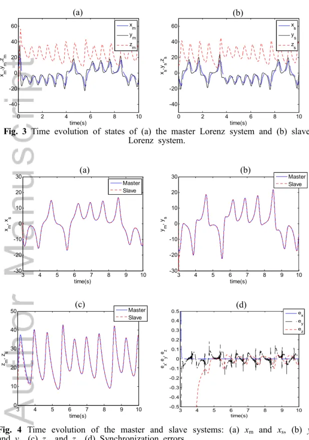
, ,b r∈ℜ are parameters.

The initial values of the master system ((xm, ym, zm) in Eq. (42)) are (xm0, ym0, zm0) = (10, 0, -10). The initial values of the slave system ((xs, ys, zs) in Eq. (43)) to be controlled are set as (xs0, ys0, zs0) = (-10, 0, 10). The state variables of the two Lorenz chaotic systems with the different initial values are shown in Fig. 3. The parameters of both Lorenz systems were selected as

σ

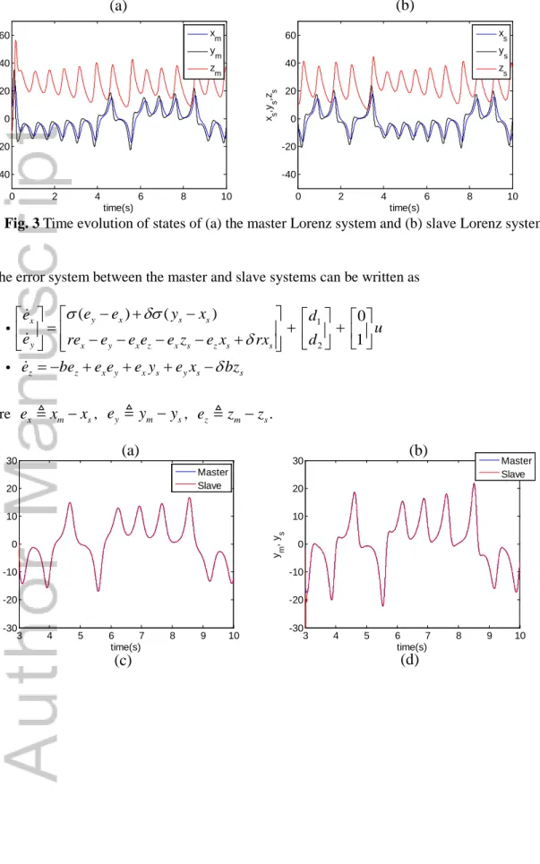
=10,r=28,b=8 / 3.

Fig. 3 Time evolution of states of (a) the master Lorenz system and (b) slave Lorenz system.

The error system between the master and slave systems can be written as

1 2 ( ) ( ) ₀ 1 y x s s x y x y x z x s z s s z z x y x s y s s e e y x e d u e re e e e e z e x rx d e be e e e y e x bz

σ

dσ

d

d

− + −         =_{ } + +   _{− − − − +}               = − + + + −      (44) where e_x x_m−x_s,

e

_y



y

_m

−

y

_s, ez zm−zs. 0 2 4 6 8 10 -40 -20 0 20 40 60 time(s) x m ,y m ,z m x m y m z m 0 2 4 6 8 10 -40 -20 0 20 40 60 time(s) x s ,y s ,z s x s y s z s 3 4 5 6 7 8 9 10 -30 -20 -10 0 10 20 30 time(s) x m , x s Master Slave 3 4 5 6 7 8 9 10 -30 -20 -10 0 10 20 30 time(s) ym , y s Master Slave

(a)

(b)

(a)

(b)

(c)

(d)

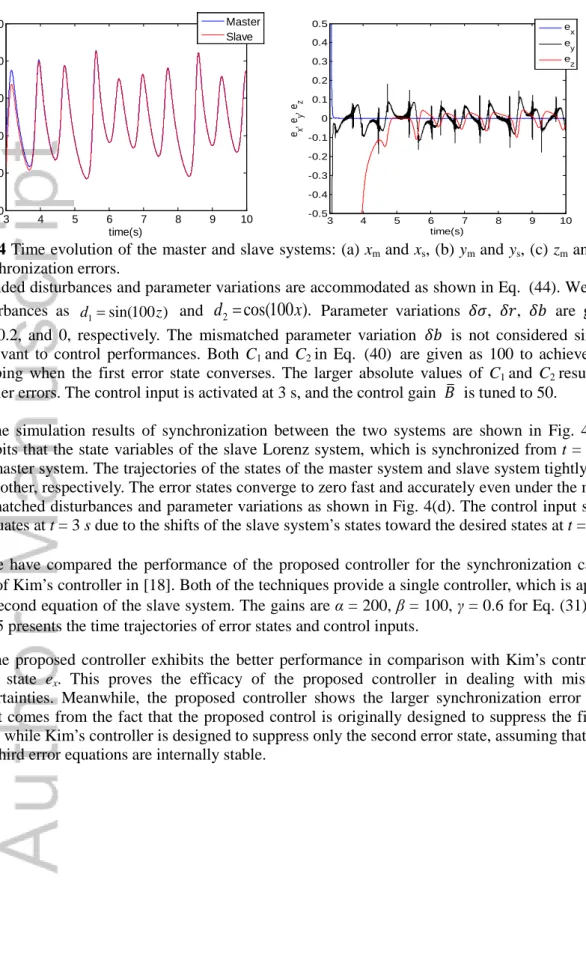
Fig. 4 Time evolution of the master and slave systems: (a) xm and xs, (b) ym and ys, (c) zm and zs. (d) Synchronization errors.

Bounded disturbances and parameter variations are accommodated as shown in Eq. (44). We assume disturbances as d₁=sin(100 )z and

d

₂

=

cos(100 ).

x

Parameter variations 𝛿𝛿𝛿𝛿, 𝛿𝛿𝛿𝛿, 𝛿𝛿𝛿𝛿 are given as 0.1, 0.2, and 0, respectively. The mismatched parameter variation 𝛿𝛿𝛿𝛿 is not considered since it is irrelevant to control performances. Both C1 and C2 in Eq. (40) are given as 100 to achieve critical damping when the first error state converses. The larger absolute values of C1 and C2 result in the smaller errors. The control input is activated at 3 s, and the control gain 𝐵𝐵� is tuned to 50.

The simulation results of synchronization between the two systems are shown in Fig. 4. Fig. 4 exhibits that the state variables of the slave Lorenz system, which is synchronized from t = 3 s with the master system. The trajectories of the states of the master system and slave system tightly overlap each other, respectively. The error states converge to zero fast and accurately even under the matched, mismatched disturbances and parameter variations as shown in Fig. 4(d). The control input suddenly fluctuates at t = 3 s due to the shifts of the slave system’s states toward the desired states at t = 3 s.

We have compared the performance of the proposed controller for the synchronization case with that of Kim’s controller in [18]. Both of the techniques provide a single controller, which is applied to the second equation of the slave system. The gains are α = 200, β = 100, γ = 0.6 for Eq. (31) in [18]. Fig. 5 presents the time trajectories of error states and control inputs.

The proposed controller exhibits the better performance in comparison with Kim’s controller for error state ex. This proves the efficacy of the proposed controller in dealing with mismatched

uncertainties. Meanwhile, the proposed controller shows the larger synchronization error ey. This

result comes from the fact that the proposed control is originally designed to suppress the first error state, while Kim’s controller is designed to suppress only the second error state, assuming that the first and third error equations are internally stable.

3 4 5 6 7 8 9 10 0 10 20 30 40 50 time(s) z m , z s Master Slave 3 4 5 6 7 8 9 10 -0.5 -0.4 -0.3 -0.2 -0.1 0 0.1 0.2 0.3 0.4 0.5 time(s) e x , e y , e z e_x e_y e_z

Fig. 5 Time evolution of (a) error state ex, (b) error state ey, (c) error state ez, and (d) control inputs under the control in [18] and the proposed control. The controllers are activated at 3 s.

4. Experiment

4.1 Regulation of the Lorenz system

In this section, we validate the proposed technique in controlling a circuit-implemented chaotic system. The Lorenz system is chosen as an example of the generalized Lorenz system. Considering the fact that the state variables of the system occupy a wide dynamic range with values that exceed the reasonable power supply limits of electric elements, we scale variables in a similar way as proposed in [11].

With the state scaling factorsx′=x/ 10, y′=y/ 10,z′=z/ 10., the Lorenz system is scaled down to

( ), 10 , 10 . x y x y rx y x z z x y bz

σ

′= ′− ′ ′= ′− −′ ′ ′ ′= ′ ′− ′    (45) The state variables have similar dynamic ranges and circuit voltages remain well within the range

of typical power supply limits. A time scaling factor should be introduced as

t

=

G

_T

t

, where

G

_T

denotes a time scaling factor. Then, the scaled system is expressed as

3 4 5 6 7 8 9 10 -0.5 -0.4 -0.3 -0.2 -0.1 0 0.1 0.2 0.3 0.4 0.5 time(s) e x u_III Proposed 4 6 8 10 -0.5 -0.4 -0.3 -0.2 -0.1 0 0.1 0.2 0.3 0.4 0.5 time(s) e y u_III Proposed 3 4 5 6 7 8 9 10 -0.5 -0.4 -0.3 -0.2 -0.1 0 0.1 0.2 0.3 0.4 0.5 time(s) e z u_III Proposed 3 4 5 6 7 8 9 10 -200 -150 -100 -50 0 50 100 150 200 time(s) u u III Proposed

(a)

(b)

(c)

(d)

{ (

)},

{

10

},

{10

}.

T T T

x

G

y

x

y

G rx

y

x z

z

G

x y

bz

σ

′

=

′

−

′

′

=

′

− −

′

′ ′

′

=

′ ′

−

′







(46)

Four operational amplifiers (LF412, National Semiconductor) and associated circuitry perform operations of sum, multiplication, and integration. Two analog multipliers (AD633, Analog Devices) implement the quadratic terms in the circuit equations. A set of state equations that govern the dynamical behavior of the circuit is obtained as

5 1 1 2 2 3 5 4 3 4 7

1

1

(

),

1

1

1

1

(

),

10

1

1

1

(

).

10

p p p

R

x

y

x

C

R

R

y

x

y

x z

C

R

R

R

z

x y

z

C

R

R

′

=

′

−

′

′

=

′

−

′

−

′ ′

⋅

′

=

′ ′

−

′

⋅







(47)

For setting

σ

=

10,

r

=

28,

b

=

8 / 3,

the resistors are selected as:

1 2

100,

3

36,

4

10,

5

1000,

6

10,

7

374 (

).

R

=

R

=

R

=

R

=

R

=

R

=

R

=

k

Ω

The capacitors are selected as

1 2 3 47

p p p

C =C =C = (nF).

The Lorenz circuit has a bandwidth of signal

x

′

in about 0 – 120Hz. The time scaling factor

G

_T

of this circuit is estimated as 22. A digital signal processor (DSP, TMS320F2812, Texas Instruments) and TMS320F28X EVM (Texas Instruments) are used for signal processing. Signal conditioning circuits are also considered for ADC input to remain in the range of 0~3V and DAC input to remain in the range of 0~4.096V. A schematic and picture of the experiment settings are shown in Figs. 6 and 7.

Fig.6 Schematic diagram of control with a DSP EVM.

Fig.7 Overall implementation for control of a chaotic circuit.

The control objective is to regulate

x

′

to 1 V. In the control law (16), the control gain 𝐵𝐵� is tuned to 90000, and

C

₁ and

C

₂ are both set as 350. The sampling frequency is set as 2 kHz to be sufficiently larger than the Nyquist frequency 240Hz, which is an upper bound on the highest frequency the signal

x

′

.

Figs.8 (a) and (b) show the waveform of the state

x

′

and the corresponding control input from the Lorenz circuit, which are measured by an oscilloscope, respectively. The control input is activated at t = 0.4. It is observed that the state

x

′

intends to converge to 1V. However, the vibration of the signal

x

′

is displayed during the steady state. The reasons that lead to the vibrations at steady state include unstable power supply to the DSP, ADC resolutions, and the external noise.

Fig.8 Experiment results: time evolution of (a) the state

x

′

and (b) control input

u

′

.

4.2 Synchronization of the Lorenz systems

Next, we conduct synchronization between two identical Lorenz circuits. Firstly, for the control input (40), the gain 𝐵𝐵� is tuned to 250000. And, both

C

₁ and

C

₂ are set as 550. And the sampling frequency is set as 3.33kHz. The experiment results show that the state

x

′

of the slave system well follows the state

x

_d

′

of the master system, as shown in Figs.9 (a) and (b). Fig. 10 displays the control input measured by an oscilloscope.

Uncertainties in the experiments result from external noise, unstable power supply to the DSP, and tolerances of the electronic elements including resistors and capacitors. In particular, in the case of synchronization, the two chaotic circuits are not exactly identical due to the tolerances that give parameter variations. The synchronization error is measured as -33mV ~ 66mV while the magnitude of the desired trajectory rises up to 2.32V. Even in the presence of those uncertainties, we observe that the proposed control achieves synchronization between the two Lorenz circuits.

(a)

(b)

Fig.10 Time evolution of states

x

_m

′

and

x

_s

′

(a) before and (b) after synchronization.

Fig.11 Time evolution of control input

u

′

for synchronization.

5. Conclusion

We have proposed a robust backstepping technique using time-delay estimation (TDE) to regulate and synchronize the Generalized Lorenz System (GLS) that contains the Lorenz system, Chen system and Lü system. The control technique provides a single controller that can be applied to any chaotic system in strict feedback form for regulation and synchronization, even if a precise model is unavailable. Mismatched uncertainties are managed by multiple TDEs. Numerical simulation results demonstrate fast, accurate and robust performance of the proposed technique in the presence of matched, mismatched disturbances and parameter variations. The proposed technique is experimentally verified with physical chaotic systems constructed by analog circuit elements. The experimental results show satisfactory performances.

1.

Chen G, Dong X.

From chaos to order: methodologies, perspectives, and applications

.

Singapore: World Scientific Pub. Co.; 1998.

2.

Andrievskii, B. R., Fradkov A. L. Control of chaos: methods and applications. II.

Applications.

Automation and Remote Control

2004;

65

(4):505–533.

3.

Chen C, Chen H. Robust adaptive neural-fuzzy-network control for the

synchronization of uncertain chaotic systems.

Nonlinear Analysis: Real World

Applications

2009;

10

(3):1466–1479.

4.

Rulkov NF, Tsimring LS. Synchronization methods for communication with chaos

over band-limited channels.

International Journal of Circuit Theory and Applications

1999;

27

(6):555–567.

5.

Chen F, Chen L, Zhang W. Stabilization of parameters perturbation chaotic system via

adaptive backstepping technique.

Applied Mathematics and Computation

2008

200

(1):101–109.

6.

Cui F et al. Bifurcation and chaos in the Duffing oscillator with a PID controller.

Nonlinear Dynamics

1997

12

(3):251–262.

7.

Gambino G, Lombardo MC, Sammartino M. Global linear feedback control for the

generalized Lorenz system.

Chaos, Solitons & Fractals

2006

29

(4):829–837.

8.

Ge SS, Wang C, Lee TH. Adaptive backstepping control of a class of chaotic systems.

International Journal of Bifurcation and Chaos

2000

10

(5):1149–1156.

9.

Layeghi H et al. Stabilizing periodic orbits of chaotic systems using fuzzy adaptive

sliding mode control.

Chaos, Solitons & Fractals

2008

37

(4):1125–1135.

10.

Liao T, Lin S Adaptive control and synchronization of Lorenz systems

Journal of the

Franklin Institute

1999

336

(6):925–937.

11.

Naseh MR, Haeri M. An optimal approach to synchronize non

‐

identical chaotic

circuits: An experimental study.

International Journal of Circuit Theory and

Applications

2011

39

(9):947–962.

12.

Noroozi N, Roopaei M, Jahromi MZ. Adaptive fuzzy sliding mode control scheme for

uncertain systems.

Communications in Nonlinear Science and Numerical Simulation

2009

14

(11):3978–3992.

13.

Yu Y, Zhang S. Adaptive backstepping synchronization of uncertain chaotic system.

Chaos, Solitons & Fractals

20014

21

(3):643–649.

14.

Wang T et al. Adaptive fuzzy backstepping control for a class of nonlinear systems

with sampled and delayed measurements.

IEEE Transactions on Fuzzy Systems

2015

23

(2):302–312.

15.

Niu Y, Wang X. A novel adaptive fuzzy sliding-mode controller for uncertain chaotic

16.

Peng C, Chen C. Robust chaotic control of Lorenz system by backstepping design.

Chaos, Solitons & Fractals

2008

37

(2):598–608.

17.

Jin M, Chang P. Simple robust technique using time delay estimation for the control

and synchronization of Lorenz systems.

Chaos, Solitons & Fractals

2009

41

(5):2672–

2680.

18.

Kim D, Gillespie RB, Chang PH. Simple, robust control and synchronization of the

Lorenz system.

Nonlinear Dynamics

2013

73

(1-2):971–980.

19.

Hsia TC, Gao LS Robot manipulator control using decentralized linear time-invariant

time-delayed joint controllers.

Proceedings IEEE International Conference on

Robotics and Automation

, 1990. 2070–2075.

20.

Kim D et al. Control and synchronization of Lorenz systems via robust backstepping

technique.

12th International Conference on Control, Automation and Systems

(ICCAS)

, 2012. 328–332.

21.

Čelikovský S, Vaněček A. Bilinear systems and chaos.

Kybernetika

1994

30

(4):403–

424.

22.

Čelikovský S, Chen G. On a generalized Lorenz canonical form of chaotic systems.

International Journal of Bifurcation and Chaos

2002

12

(8):1789–1812.

23.

Lorenz EN. Deterministic nonperiodic flow.

Journal of the Atmospheric Sciences

1963

20

(2):130–141.

24.

Chen G, Ueta T. Yet another chaotic attractor.

International Journal of Bifurcation and

Chaos

1999

9

(7):1465–1466.

25.

Lü J, Chen G. A new chaotic attractor coined.

International Journal of Bifurcation and

Chaos

2002

12

(3):659–661.

26.

Chen D et al. Circuit implementation and model of a new multi

‐

scroll chaotic system.

International Journal of Circuit Theory and Applications

2014

42

(4):407–424.

27.

Li Y, Tang WKS, Chen G. Hyperchaos evolved from the generalized Lorenz equation.

International Journal of Circuit Theory and Applications

2005

33

(4):235–251.

28.

Li Y et al. A new hyperchaotic Lorenz

‐

type system: generation, analysis, and

implementation.

International Journal of Circuit Theory and Applications

2011

39

(8):

865–879.

29.

Jafari S, Haeri M, Tavazoei MS. Experimental study of a chaos-based communication

system in the presence of unknown transmission delay.

International Journal of

Circuit Theory and Applications

2010;

38

(10):1013–1025.

30.

Park C, Lee C, Park M. Design of an adaptive fuzzy model based controller for chaotic

dynamics in Lorenz systems with uncertainty.

Information Sciences

2002

147

(1): 245–

266.

Control

1997

7

(2): 143–154.

32.

Wu Z et al. Sampled-data fuzzy control of chaotic systems based on a T–S fuzzy

model

IEEE Transactions on Fuzzy Systems

2014

22

(1):153–163.

33.

Zhang L et al. Fuzzy adaptive synchronization of uncertain chaotic systems via

delayed feedback control.

Physics Letters A

2008

372

(39):6082–6086.

34.

Čelikovský S Chen G. On the generalized Lorenz canonical form.

Chaos, Solitons &

Fractals

2005 26(5):1271–1276.

35.

Wang Y et al. Adaptive synchronization of GLHS with unknown parameters.

International Journal of Circuit Theory and Applications

2009 37(8):920–927.

36.

Wu X, Cai J, Zhao Y. Some new algebraic criteria for chaos synchronization of Chua's

circuits by linear state error feedback control.

International Journal of Circuit Theory

and Applications

2006 34(3):265–280.

37.

Youcef-Toumi K, Ito O, A time delay controller for systems with unknown dynamics.

Journal of Dynamic Systems Measurement and Control

1990 112(1):133–142.

38.

Hsia TC, Lasky TA, Guo Z. Robust independent joint controller design for industrial

robot manipulators.

IEEE Transactions on Industrial Electronics

, 1991

38

(1):21–25.

39.

Jin M, Lee J, Chang PH, Choi C. Practical nonsingular terminal sliding-mode control

of robot manipulators for high-accuracy tracking control.

IEEE Transactions on

Industrial Electronics

, 2009

56

(9):3593–3601.

40.

Jin M, Kang SH, Chang PH. Robust compliant motion control of robot with nonlinear

friction using time-delay estimation.

IEEE Transactions on Industrial Electronics

,

2008

55

(1):258–269.

41.

Jin M, Lee J, Tsagarakis N. Model-free robust adaptive control of humanoid robots

with flexible joints.

IEEE Transactions on Industrial Electronics

, 2017

64

(2):1706–

1715.

42.

Lee J, Jin M, Ahn KK. Precise tracking control of shape memory alloy actuator

systems using hyperbolic tangential sliding mode control with time delay estimation.

Mechatronics

, 2013

23

(3):310–317.

43.

Jin M, Lee J, Ahn KK. Continuous nonsingular terminal sliding-mode control of shape

memory alloy actuators using time delay estimation. IEEE/ASME

Transactions on

Mechatronics

2015

20

(2):899–909.

44.

45.

Jin Y et al. Stability guaranteed time delay control of manipulators using nonlinear

damping and terminal sliding mode

IEEE Transactions on Industrial Electronics

, 2013

60

(8):3304–3317.

Wang Q et al. Theoretical Design and FPGA-Based Implementation of

Higher-Dimensional Digital Chaotic Systems IEEE Transactions on Circuits and Systems I,

2016 63(3):401–412.

0 2 4 6 8 10 -30 -20 -10 0 10 20 30 40 50 60 time(s) x, y, z x y z 0 2 4 6 8 10 -30 -20 -10 0 10 20 30 40 50 60 time(s) x, y, z x y z 0 2 4 6 8 10 -5 -4 -3 -2 -1 0 1 2 3 4 5x 10 -3 time(s) e 1 Under d 1 Under d 1 & d2 0 2 4 6 8 10 -200 -100 0 100 200 300 400 time(s) C o n tr o l in p u t Under d 1 Under d 1 & d2

Fig. 1 Responses of the Lorenz system in the presence of (a) a matched disturbance and (b) matched and mismatched disturbances. The time evolution of

(c) error states e1 and (d) control inputs u for the two cases. The control input

is exerted at time 5 s. 0 2 4 6 8 10 -20 -10 0 10 20 30 time(s) x data1 data2 data3 0 2 4 6 8 10 -200 -100 0 100 200 300 400 500 600 time(s) C o n tr o l in p u t data1 data2 data3 (b) (a) (c) (d) (a) Kim (b) Jin Proposed Kim Jin Proposed

0 2 4 6 8 10 -40 -20 0 20 40 60 time(s) x m ,y m ,z m x m y m z m 0 2 4 6 8 10 -40 -20 0 20 40 60 time(s) x s ,y s ,z s x s y s z s

Fig. 3 Time evolution of states of (a) the master Lorenz system and (b) slave Lorenz system. 3 4 5 6 7 8 9 10 -30 -20 -10 0 10 20 30 time(s) x m , x s Master Slave 3 4 5 6 7 8 9 10 -30 -20 -10 0 10 20 30 time(s) y m , y s Master Slave 3 4 5 6 7 8 9 10 0 10 20 30 40 50 time(s) z m , z s Master Slave 3 4 5 6 7 8 9 10 -0.5 -0.4 -0.3 -0.2 -0.1 0 0.1 0.2 0.3 0.4 0.5 time(s) e x , e y , e z e_x e_y e_z

Fig. 4 Time evolution of the master and slave systems: (a) xm and xs, (b) ym

and y, (c) z and z. (d) Synchronization errors.

(a) (b)

(a) (b)

3 4 5 6 7 8 9 10 -0.5 -0.4 -0.3 -0.2 -0.1 0 0.1 0.2 0.3 0.4 0.5 time(s) e x u_III Proposed 4 6 8 10 -0.5 -0.4 -0.3 -0.2 -0.1 0 0.1 0.2 0.3 0.4 0.5 time(s) e y u_III Proposed 3 4 5 6 7 8 9 10 -0.5 -0.4 -0.3 -0.2 -0.1 0 0.1 0.2 0.3 0.4 0.5 time(s) e z u_III Proposed 3 4 5 6 7 8 9 10 -200 -150 -100 -50 0 50 100 150 200 time(s) u u III Proposed

Fig. 5 Time evolution of (a) error state ex, (b) error state ey, (c) error state ez,

and (d) control inputs under the control in [18] and the proposed control. The

controllers are activated at 3 s.

(a) (b)

Fig.7 Overall implementation for control of a chaotic circuit.

Fig.8 Experimental results: time evolution of (a) state

x

¢

and (b) control input u¢.

(a) _(b)

The proposed control provides synergy through the combination of the backstepping control and time-delay estimation (TDE) technique. TDE is used to estimate and cancel nonlinearities and uncertainties, and the backstepping method is adopted to provide robustness against matched and mismatched uncertainties.

DSP EVM

Control input

ADC

DAC

Chaotic circuit

State

x’

conditioning

circuit

Control input

conditioning

circuit

(

_out

)

u

¢ =

p V

-

q

3V

0V

3V

0V

4095

0

4.095V

0V

2V

out

V

0 1 2 3 4 5 -5 0 5 time(sec) x, y, z State variables x

4095

0

0V

B

V

(

)

in

V

=

A x

¢

+

B

in

V

u

G u

¢

x

¢

x

¢

p

´

q

V

1000 p ´