Sequential quadratic programming-based fast path planning algorithm
subject to no-fly zone constraints
Article in Engineering Optimization · December 2015
DOI: 10.1080/0305215X.2015.1111085 CITATIONS 0 READS 98 6 authors, including:
Some of the authors of this publication are also working on these related projects: Optimization of Power Systems with Voltage Security ConstraintsView project Mingwei Sun Nankai University 61 PUBLICATIONS 293 CITATIONS SEE PROFILE Haidong Yi Nankai University 1 PUBLICATION 0 CITATIONS SEE PROFILE Zenghui Wang
University of South Africa 97 PUBLICATIONS 558 CITATIONS
SEE PROFILE
Zengqiang Chen
Beijing Institute of Petrochemical Technology 289 PUBLICATIONS 3,566 CITATIONS
SEE PROFILE
All content following this page was uploaded by Haidong Yi on 22 February 2016. The user has requested enhancement of the downloaded file.
Full Terms & Conditions of access and use can be found at
http://www.tandfonline.com/action/journalInformation?journalCode=geno20
Download by: [Nankai University], [Haidong Yi] Date: 03 December 2015, At: 04:49
Engineering Optimization
ISSN: 0305-215X (Print) 1029-0273 (Online) Journal homepage: http://www.tandfonline.com/loi/geno20
Sequential quadratic programming-based fast
path planning algorithm subject to no-fly zone
constraints
Wei Liu, Shunjian Ma, Mingwei Sun, Haidong Yi, Zenghui Wang & Zengqiang
Chen
To cite this article: Wei Liu, Shunjian Ma, Mingwei Sun, Haidong Yi, Zenghui Wang & Zengqiang Chen (2015): Sequential quadratic programming-based fast path planning algorithm subject to no-fly zone constraints, Engineering Optimization
To link to this article: http://dx.doi.org/10.1080/0305215X.2015.1111085
Published online: 03 Dec 2015.
Submit your article to this journal
View related articles
http://dx.doi.org/10.1080/0305215X.2015.1111085
Sequential quadratic programming-based fast path planning
algorithm subject to no-fly zone constraints
Wei Liua,b, Shunjian Maa, Mingwei Suna∗, Haidong Yia, Zenghui Wangcand Zengqiang Chena
aDepartment of Automation and Intelligent Science, College of Computer and Control Engineering,
Nankai University, Tianjin, PR China;bUnit 62214, PLA, PR China;cDepartment of Electrical and
Mining Engineering, University of South Africa, Florida, South Africa (Received 31 March 2015; accepted 16 October 2015)
Path planning plays an important role in aircraft guided systems. Multiple no-fly zones in the flight area make path planning a constrained nonlinear optimization problem. It is necessary to obtain a feasible optimal solution in real time. In this article, the flight path is specified to be composed of alternate line segments and circular arcs, in order to reformulate the problem into a static optimization one in terms of the waypoints. For the commonly used circular and polygonal no-fly zones, geometric conditions are established to determine whether or not the path intersects with them, and these can be readily pro-grammed. Then, the original problem is transformed into a form that can be solved by the sequential quadratic programming method. The solution can be obtained quickly using the Sparse Nonlinear OPTi-mizer (SNOPT) package. Mathematical simulations are used to verify the effectiveness and rapidity of the proposed algorithm.
Keywords: path planning; SNOPT; nonlinear programming; no-fly zone; polygon; intersection point
1. Introduction
Path planning has been widely applied in aircraft guided systems (Hwang and Ahuja1992). Its main objective is to find an optimal path from the start point to the end point subject to multiple constraints about direction, range, time and avoidance of obstacles according to the dynamic capability of specific flight vehicles (Moon and Kim2005). Many of these constraints are difficult to deal with in practice (Chandler, Rasmussen, and Pachter2000). For example, the impact time is a crucial factor in a salvo attack against a highly valued warship equipped with advanced air defence installations such as close-in weapon systems. In a salvo attack, the anti-ship missiles should impact a warship simultaneously from different directions, which makes the impact time an important factor in achieving good performance. For civil aircraft, the time factor is also vital because the landing time is scheduled so tightly that it is difficult to change the arrangements. In the realm of path planning, the main obstacles generally include threat zones and no-fly zones. Compared with other constraints, the no-fly zone constraint needs to be specifically considered in the path planning process. Generally speaking, no-fly zones are specific areas that cannot be passed through. Typical no-fly zones in peacetime include lightning areas and complex terrains which jeopardize normal flight. In wartime, no-fly zones may cover adversaries’ firing locations,
*Corresponding author. Email:[email protected]
© 2015 Taylor & Francis
hostile detection positions and densely populated areas. For sea-skimming anti-ship missiles, a particular kind of no-fly zone is caused by scattered islands, which make the on-board radar altimeter unavailable so that reliable flight cannot be achieved. A lot of progress has been made in dealing with the impact time and angle specifications (Kim and Gilder1973; Lee, Jeon, and
Tahk2007; Wilson1963). However, these methods are unable to deal with no-fly zones directly.
In the past few decades, considerable effort has been devoted to sophisticated path plan-ning algorithms, such as the Gauss pseudospectral method (GPM) (Zhanget al.2014), genetic
algorithm (GA) (Smierzchalski1999), probabilistic roadmap method (PRM) (Overmars1992)
and A* method (Korf1985). Although these approaches have illustrated their effectiveness, their huge computational complexity is unavoidable and extensive memory is required. For example, a high-order interpolation polynomial (even nearly a hundredth order) is indispensable for the GPM, which is difficult to implement in reality and lacks flexibility; and both the memory and the optimization time for the A* method will increase exponentially when the search area is expanded. Meanwhile, artificial intelligence-based methods, such as GA and particle swarm opti-mization (PSO) (Liet al.2014), have many parameters that need to be tuned to obtain satisfactory solutions, and this strongly depends on the skill and experience of operators in a trial-and-error process. For the A* method, the selection of heuristic functions is also a shortcoming. PRM is a useful path planning method; however, the generated path is a graph composed of stiffly con-nected line segments, which cannot meet the dynamic requirements of a flight vehicle. Therefore, an efficient and practical path planning algorithm subject to multiple no-fly zone constraints is urgently needed for practitioners.
In practice, the simplest and traditional forms of paths, combining line segments and tangential circular arcs, are preferred since these forms can be readily set on-board by changing only the cor-responding parameters of the waypoints. Compared with other path modelling approaches such as polynomial approaches, this line–arc approach exhibits its simplicity and flexibility with lower memory requirements, and the programming procedure of this approach is simple (Fu, Ding, and
Zhou2012; Guo, Fan, and Ma2008; Helgason, Kennington, and Lewis2001). Therefore, the
line–arc method is acceptable to practitioners.
In this article, a fast path planning algorithm is proposed based on the conventional forms of alternate combinations of line segments and circular arcs, subject to circular and polygonal no-fly zones. The major contribution is that the no-no-fly zone avoidance problem is reformulated into a set of explicit constraints. Therefore, the nonlinear programming method can be implemented in a straightforward and fast manner. Thereafter, it can be solved directly by means of the mature and reliable Sparse Nonlinear OPTimizer (SNOPT) software package. Mathematical simulations will be used to verify the effectiveness and speed of the proposed algorithm.
The remaining parts of the article are organized as follows. In Section2, a planar path planning model is presented and constraints are also considered while formulating the research objec-tive. Then, the no-fly zone constraints and their corresponding intersection judging schemes
are proposed in Section 3. The SNOPT package is used to solve the path planning problem
in Section4. The mathematical simulation results and their analyses are provided in Section5. The conclusions are summarized in Section6.
2. Kinetic model and constraints for path planning 2.1. Kinetic model of unmanned aerial vehicles A planar path planning model can be described as
˙
x=Vcosγ
˙
y=Vsinγ (1)
˙
γ =a/V
where(x, y)are the position coordinates of a flight vehicle,γ is the flight path angle,a is the
normal acceleration, which is perpendicular to the velocity and drives the missile to change direction, anda=V2/r, whereris the turning radius. An aerodynamic force proportional toais
then needed to generate such movement. It implies that a smallerrrequires a larger aerodynamic force, which is more difficult to obtain or may damage the structure of the airframe.
Assume that the velocityVis constant. In the literature, a constant velocity is commonly used in the path planning problem (Jeon, Lee, and Tahk2006; Lee, Jeon, and Tahk2007) since path planning methods are mostly applied to civil and combat aircrafts and cruise missiles during their cruise flight. Moreover, the closed-loop velocity control is normally adopted to maintain an approximately constant velocity value as accurately as possible. However, the practical velocity may vary from the nominal value owing to diverse perturbations, such as wind, temperature and control errors. Here,V is assumed to be the lower bound of possible realistic values. Therefore, the flight vehicle can properly perform a weak manoeuvre around the line segment of the nom-inal flight path to consume the excessive flight time (Zhang and Ma2008). This is a traditional strategy utilized online, which is beyond the scope of this work. It should be noted that such velocity variations are not very large, and hence minor manoeuvres can readily be planned to meet the flight time requirements without any impact on the no-fly zones. In other words, the aim here is to attempt to provide a basic path to follow while the realistic one operates around it to attenuate the perturbations.
There is also another factor resulting in variable velocity. In the landing phase, a civil passen-ger aircraft should reduce actively its velocity in a preprogrammed way before its final landing, to ensure safety. In this case, because this active deceleration phase is rather short for a specified trajectory, its time consumption can be precalculated and eliminated from the total path. In this way, the remaining work is to plan a path before the start of the deceleration phase, which falls within the framework. The objective of path planning is to minimize the cost function
J =1
2 ! tf
t0
a2dt (2)
with the boundary conditions as
x(t0)=x0, y(t0)=y0, γ(t0)=γ0 (3)
x(tf)=xf, y(tf)=yf, γ(tf)=γf (4)
wheret0is the initial time,(x0, y0)is the initial position,γ0is the initial flight path angle,(xf, yf)
is the terminal position, γf is the specified terminal flight path angle, and tf is the specified
flight time. The normal acceleration represents the manoeuvrability of a flight vehicle. The cost function (2) implies that a low curvature path is favourable to maintain safety and reduce fuel consumption. This optimization problem can be mathematically formulated as a nonlinear opti-mal control problem, and it is impossible to obtain its analytical solution owing to its complexity and no-fly zone constraints.
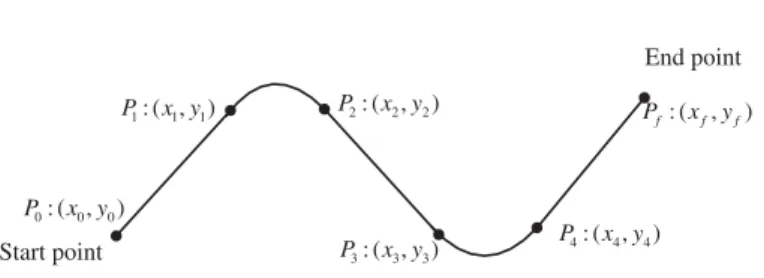
In this optimization problem, the desired path is composed of line segments and circular arcs in turn, as shown in Figure1, where(xi, yi)(i=0, . . ., f)are waypoints. There aremcircular
arcs, andf =2m+1. The line segments are tangential to the adjacent circular arcs to guarantee that the velocity direction is smooth. Because the velocity is constant, the range constraint is equivalent to the flight time constraint.
Therefore, a static nonlinear programming problem can be obtained, and its programming variables are the coordinates of the waypoints.
0: ( , )0 0 P x y 1: ( , )1 1 P x y P2: ( , )x y2 2 3: ( , )3 3 P x y : ( , ) f f f P x y 4: ( , )4 4 P x y Start point End point
Figure 1. Simplified planar path planning model.
2.2. Constraints of the optimization The constraints include:
(1) Flight time
The length of the flight path is represented as
m " i=1 riθi+ m " i=0 # (x2i−x2i+1)2+(y2i−y2i+1)2=Ls (5)
whereLsis the specified path length and
ri= $ (xoi−x2i−1)2+(yoi−y2i−1)2 (6) θi=2 arcsin % |P2i−1P2i| 2ri & (7) xoi = (y2i−1−y2i−2)[x22i−1−x22i−(y2i−1−y2i)2]−2x2i−1(x2i−1−x2i−2)(y2i−1−y2i) 2[(x2i−1−x2i)(y2i−1−y2i−2)−(x2i−1−x2i−2)(y2i−1−y2i)] (8) yoi = (x2i−1−x2i−2)[(x2i−1−x2i)2+y22i−y22i−1]+2y2i−1(y2i−1−y2i−2)(x2i−1−x2i) 2[(x2i−1−x2i)(y2i−1−y2i−2)−(x2i−1−x2i−2)(y2i−1−y2i)] and |P2i−1P2i| = # (y2i−1−y2i)2+(x2i−1−x2i)2 (9)
(2) Initial and impact angles The initial angle constraint is
arctan %y 1−y0 x1−x0 & =γ0 (10)
and the terminal impact angle constraint is arctan %y f −y2m xf −x2m & =γf (11)
(3) Maximum turning angle
The airframe structure and the operational requirements of the engine limit the turning capability of a flight vehicle. This constraint can be described as
ri≥rc, i=1, 2, . . ., m (12)
wherercis a given radius.
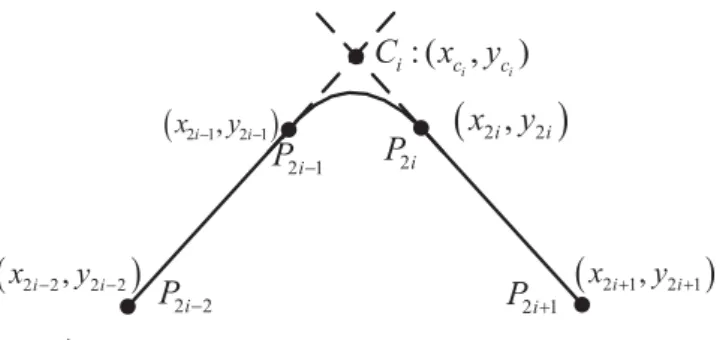
Figure 2. Tangency constraint. (4) Tangency constraint
The adjacent line segment and arc should be tangential to each other to ensure the con-tinuity of the velocity direction. Denote the intersection point between the extensions of line segmentsP2i−2P2i−1andP2iP2i+1asCi(i=1, 2, . . ., m). Hence,|P2i−1Ci| = |CiP2i|is
necessary to ensure the adjacent condition, as shown in Figure2, where
|P2i−1Ci| = $ (y2i−1−yci)2+(x2i−1−xci)2 |CiP2i| = $ (yci−y2i)2+(xci−x2i)2 (13) and xci = x2i−2(x2i−x2i+1)(y2i−1−y2i−2)−x2i+1(x2i−1−x2i−2)(y2i−y2i+1) −(x2i−1−x2i−2)(x2i−x2i+1)(y2i−2−y2i+1) (x2i+1−x2i)(y2i−1−y2i−2)−(x2i−1−x2i−2)(y2i+1−y2i) yci = y2i+1(x2i−x2i+1)(y2i−1−y2i−2)−y2i−2(x2i−1−x2i−2)(y2i−y2i+1) −(y2i−1−y2i−2)(y2i−y2i+1)(x2i−2−x2i+1) (x2i+1−x2i)(y2i−1−y2i−2)−(x2i−1−x2i−2)(y2i+1−y2i) (14)
(5) No-fly zones constraint
This article mainly focuses on how to handle no-fly zone constraints, especially circular and polygonal no-fly zones. More detail will be presented in the next section.
3. Simplifications of no-fly zone constraints 3.1. Circular no-fly zones
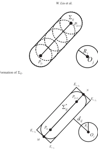
Consider thejth circular no-fly zone(j=1, 2, . . ., n#), which is centred atOjwith a radius of
Rj, as shown in Figure3and indicated as#j. The condition is sought that ensures that a particular
edge ofP2iP2i+1has no intersection point with#j.
Figure 3. Circular no-fly zone.
Figure 4. Formation of$ij.
Figure 5. Formation of'∗ ijfrom$ij.
Denote a virtual circle as#′j, which is centred atP2iwith a radius ofRj. The centre of#′jis
moved toP2i+1, just along the edgeP2iP2i+1. In this process, the envelope of dynamic circles is
shown in Figure4as the dashed line, which is represented by$ij. According to Figure3, it is
clear that the edgeP2iP2i+1will not intersect with#jif and only ifOj is not contained in$ij.
Therefore, one has:
Condition 1: Ojis not contained in$ij.
It is apparent that Condition 1 is a sufficient and necessary condition. To further facilitate practical programming, an extended rectangle'∗
ijis used instead of$ij,
as shown in Figure5. Then, one has:
Condition 2: Ojis not contained in'∗ij.
It should be noted that Condition 2 is only a sufficient condition to guarantee no intersection between#jandP2iP2i+1. In other words, the feasible solution may be dropped using this
con-dition. However, this has only a small possibility, according to extensive simulations carried out by the authors.
For each#j (j=1, 2, . . ., n)and each edgeP2iP2i+1 (i=0, 1, . . ., m)in the flight path,
Condition 2 can be described as
dij(x2i, y2i, x2i+1, y2i+1) >0, i=0, 1, . . ., m; j=1, 2, . . ., n (15)
wheredijdenotes the minimal distance fromOjto$ij∗.
Figure 6. Polygonal no-fly zone.
Figure 7. Formation of$ijfrom the polygonal no-fly zone.
3.2. Polygonal no-fly zones
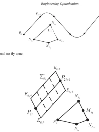
In reality, the polygon is much more frequently used to represent no-fly zones owing to its irreg-ular nature. For thejth polygonal no-fly zone (j=1, 2, . . ., n() withTj edges indicated as
Nj1Nj2· · ·NjTj and denoted as
(
j, as shown in Figure6, the condition is sought that guarantees
that each line segmentP2iP2i+1has no intersection point with(j, which is equivalent to the
con-dition thatP2iP2i+1does not intersect with each edge of(j, and meanwhile bothP2iandP2i+1
are outside(j.
This task can be accomplished by judging the relationship of a set of line segments, thus obtaining the following two conditions:
Condition 3: P2iP2i+1does not intersect with each edge of(j.
Condition 4: P2iandP2i+1are not contained in(j.
To make the program more efficient in using SNOPT and also to simplify Condition 3, the follow-ing method, shown in Figure7, can be used to judge the relationship between two line segments, whereMjk (k=1, 2, . . ., Tj)is the midpoint of NjkNjk+1 (whereNjTj+1 =Nj1), thekth edge of (
j. Suppose thatNjkNjk+1is moved toEijk4Eijk1in parallel with its midpointMjkoverlapping with
P2i. Then, this line is moved toP2i+1, just along the line segmentP2iP2i+1, and a parallelogram
region'∗ijk can be obtained. According to Figure6, it is clear that the edge P2iP2i+1 will not
intersect withNjkNjk+1if and only ifMjk is not contained in
'∗
ijk, which can be formulated as:
Condition 5: Mjk is not contained in
'∗
ijk.
For each(j(j=1, 2, . . ., n()and each edgeP2iP2i+1 (i=0, 1, . . ., m)in the flight path,
Condition 4 can be described as
lij(xi, yi) >0, i=1, 2, . . ., f −1; j=1, 2, . . ., n( (16)
Figure 8. The circular arc is contained tightly in a rectangle%i. and Condition 5 can be described as
dijk(x2i, y2i, x2i+1, y2i+1) >0, i=0, 1, . . ., m; j=1, 2, . . ., n(; k=1, 2, . . ., Tj
(17) where lij denotes the distance from the ith waypoint to the jth polygon, and dijk denotes the distance from the midpoint of thekth edge in thejth polygon no-fly zonesMjk to$ij∗k.
3.3. No-fly zones and circular arcs
So far, only the line segments in the trajectory have been taken into account when considering the no-fly zones, which implies that there may be intersections between the circular arcs and the no-fly zones under certain circumstances. It is reasonable to focus on the line segments because they generally play a dominant role in the flight path in terms of total length. The circular arcs are neglected in the presence of no-fly zones in order to speed up the rate of convergence and find feasible solutions with fewer constraints. Next, the case of a circular arc is investigated further to make the result more accurate.
Considering theith circular arcP!2i−1P2i(i=1, 2,!,m)in the flight path and thejth circular
no-fly zone#j(j=1, 2,!,n#)or thejth polygonal no-fly zone (
j(j=1, 2,!,n(), a
simpli-fied judging condition is sought to investigate the relationship betweenP!2i−1P2iand#j or(j.
The core is to use a rectangle to approximate a circular arc in order to utilize the methods of judging the relationship between the no-fly zones and line segments mentioned earlier.
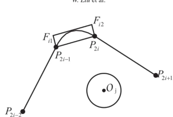
First, the circular arc can be contained tightly in a rectangleP2i−1P2iFi2Fi1, indicated as%iin
Figure8, where xFi1 =x2i−1+ %x 2i−1+x2i 2 −xoi & Ki (18) yFi1 =y2i−1+ %y 2i−1+y2i 2 −yoi & Ki (19) xFi2 =x2i+ %x 2i−1+x2i 2 −xoi & Ki (20) yFi2 =y2i+ %y 2i−1+y2i 2 −yoi & Ki (21)
and the scale factorKiis given as
Ki=
ri
#
((x2i−1+x2i/2)−xoi)2+((x2i−1+x2i/2)−xoi)2
−1 (22)
If there is no intersection between%iand the no-fly zone, there will be no intersection between
the circular arcP!2i−1P2iand the no-fly zone.
Condition 6:%idoes not intersect with#jor(j.
It should be noted that Condition 6 is also a sufficient condition to guarantee no intersection betweenP!2i−1P2iand#jor(j.
Secondly, the line segments ofP2i−1P2i,P2iFi2,Fi2Fi1 andFi1P2i−1 are taken as augmented
line segments of the trajectory to utilize the judging method proposed in Sections 3.1 and3.2 to deal with circular and polygonal no-fly zones, respectively. To cancel excessive overlap and unnecessary judging regions,%iis simplified into two line segmentsP2i−1P2iandFi1Fi2, which
almost cover the entire judging regions when employed.
Condition 7: P2i−1P2iandFi1Fi2do not intersect with#jor(j.
It should be noted that it is not necessary to apply Condition 7 to all no-fly zones and circular arcs, to eliminate the conservativeness of this extended constraint. It is a complementary strategy, used when the method, which only considers the line segment constraints, fails to generate a feasible solution. In this case, the corresponding arcs which intersect with the no-fly zones can be added as supplementary constraints until a feasible solution is found. Therefore, the arcs do not need to be incorporated all together, thus reducing the computational complexity.
4. Nonlinear programming solver 4.1. Sequential quadratic programming
Sequential quadratic programming (SQP) was proposed by Wilson (1963) and gradually improved by Han (1976,1977), Powell (1978) and others, and is usually denoted as the Wilson– Han–Powell algorithm. Chamberlainet al. (1982) completed this improvement process to show that the SQP method is not only global convergent but also locally superlinearly convergent. Therefore, SQP has become one of the most effective algorithms used to solve nonlinear constrained optimization problems (Kim and Kim2014; Roh and Kim2002).
A typical nonlinear programming problem can be formulated as minfobj(x)
s.t. hi(x)=0, i=1, 2, . . ., neq
gj(x)≥0, j=1, 2, . . ., nineq
(23)
wherefobj(x)is the cost function, andhi(x)andgj(x)are the equality and inequality constraints,
respectively. The problem can be materialized by a Lagrangian function as
L(x, λ)=fobj(x)+ neq " i λihi(x)+ nineq " j µjgj(x) (24)
whereλiandµjare the Lagrangian multipliers. The Hessian matrix of the Lagrangian function
is Hk=Hk−1+ qkqTk qT ksk − Hk−1sksTkHk−1 sT kHk−1sk (25) where sk=xk−xk−1 (26)
qk=fobj(xk)+ neq " i λihi(xk)+ nineq " j µjgj(xk)−fobj(xk−1)− neq " i λihi(xk−1)− nineq " j µjgj(xk−1) (27)
In the course of optimization, the following approximated quadratic sub-problem is solved to ensure the monotonic descent of the objective function at each step in order to approach the feasible solution: min %1 2'x TH k'x+∇fobj(xk)T'x & s.t. hi(xk)+∇hi(xk)T'x=0, 'x=0 gj(xk)+∇gj(xk)T'x≥0, 'x≥0 (28)
According to the optimization of (28), the search direction'xkcan be obtained, and thenxk+1=
xk+αk'x, where αk∈(0, 1) denotes the step size. The iteration repeats until the desirable
convergence condition, the Karush–Kuhn–Tucker (KKT) condition, is satisfied. Therefore, the optimal solution to the nonlinear programming problem can be obtained.
4.2. SNOPT
SNOPT is a reliable constrained nonlinear programming solver that was designed to implement the SQP algorithm. SNOPT exhibits excellent performance in large-scale optimization problems and performs best in cases with a moderate number of variables (Gill, Murray, and Saunders 2008).
The source code of SNOPT is in Fortran. Therefore, SNOPT has strong portability and flexi-bility, and offers interfaces including Fortran, C/C+ + and MATLAB, that can be used by most compilers. An effective method is used to compute the distance from a point to a polygon by computing the minimal distance from this point to each edge of the polygon (MATLAB
Cen-tral 2008). It was originally developed in MATLAB and later rewritten in C+ + for higher
efficiency. Here, C+ + is used to realize the function of Section3(the code is available upon request).
5. Mathematical simulation
The following mathematical simulations are provided to validate the effectiveness and the computational cost of the proposed algorithm.
5.1. Simulations without arc intersection judgement
The overall scenario parameters are provided in Table1. The simulations are performed using
a desktop computer with core i3 CPU, 4 GB memory and Windows 8.1. C+ + language is
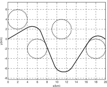
utilized to realize this computer simulation. The corresponding results are shown in Figures9– 14, where the dashed areas are the no-fly zones. Notice that all these optimizations are carried out without using the judgement between no-fly zones and circular arcs. The proposed algorithm can solve the path planning problems within 1 s. It can be seen that the optimal solutions can be obtained quickly even though there are multiple kinds of no-fly zone, which means that the proposed method can be implemented in real time. Moreover, this algorithm can deal with not only convex polygons but also concave polygons, which is very important for practical problems.
Table 1. Simulation parameters I.
P0(km) Pf (km) ϕ0(deg) ϕf(deg) Ls(km) Computational time (s)
Figure 9 (0, 0) (20, 0) 30 −30 30 0.10 Figure10 (0, 0) (20, 0) 30 −30 30 0.19 Figure11 (0, 0) (30, 0) 30 −20 40 0.19 Figure12 (0, 0) (20, 0) 30 −30 30 0.63 Figure13 (0, 0) (30, 0) 30 −30 50 0.16 Figure14 (0, 0) (20, 0) 30 −40 40 0.28
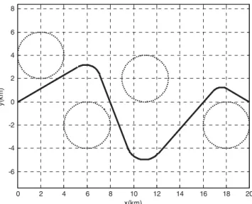
Figure 9. Path planning with three circular no-fly zones.
Figure 10. Path planning with four circular no-fly zones.
Figure 11. Path planning with three polygonal no-fly zones.
Figure 12. Path planning with four polygonal no-fly zones.
5.2. Simulations with arc intersection judgement
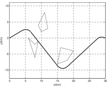
However, owing to the lack of judgement between no-fly zones and circular arcs, there is a deficiency, as shown in Figure15, where one of the arcs in the path has collided with a no-fly zone. This is because, to speed up convergence, the intersection between the circular arcs and the no-fly zones is not taken into account. In common scenarios, this simplified optimization may be conducted because the major parts of a feasible path are normally line segments. In the case of this problem, the judgement conditions for the circular arcs should be considered. With Condition 7 added, the result is shown in Figure16, where the undesired collision can be eliminated completely. Furthermore, this enhancement can be illustrated by another example, shown in Figure17. The overall scenario parameters are presented in Table2.
Figure 13. Path planning with two polygonal and one circular no-fly zones.
Figure 14. Path planning with two polygonal and two circular no-fly zones.
5.3. Comparative simulations
There are many algorithms in the realm of path planning. The traditional methods to avoid no-fly zones are based on geometric characteristics. However, to the authors’ knowledge, all these strategies can only guarantee that the upper bound of flight time is less than a specific value, rather than being strictly equal to this value in the process of regulating the path. This shortcom-ing does not exist in the proposed method because the flight time is a hard constraint embedded in the optimization.
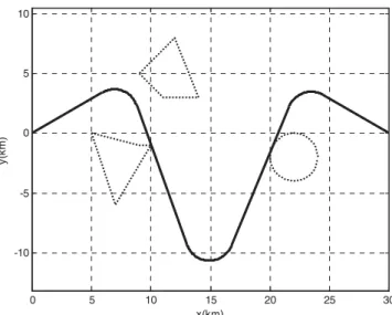
In recent years, artificial intelligent optimization methods have played an active role in path planning. Diverse constraints can be formulated in a unified way without remarkable distinctions. GA and PSO are two typical representatives of this kind of algorithm. Here, PSO- and GA-based path planning methods are applied to the same scenario in Figure10, where the flight range and
0 2 4 6 8 10 12 14 16 18 20 -8 -6 -4 -2 0 2 4 6 x(km) y(km) 0 5 10 15 20 25 30 -15 -10 -5 0 x(km) y(km) (a) (b)
Figure 15. Undesired path planning. (a) Path planning with circular no-fly zones; (b) path planning with polygonal no-fly zones. 0 2 4 6 8 10 12 14 16 18 20 -8 -6 -4 -2 0 2 4 6 x(km) y( km ) 0 5 10 15 20 25 30 -15 -10 -5 0 5 10 x(km) y( km ) (a) (b)
Figure 16. Improved path from Figure 15. (a) Path planning with circular no-fly zones; (b) path planning with polygonal no-fly zones.
0 2 4 6 8 10 12 14 16 18 20 -6 -4 -2 0 2 4 6 x(km) y( km ) 0 2 4 6 8 10 12 14 16 18 20 -6 -4 -2 0 2 4 6 x(km) y( km ) (a) (b)
Figure 17. Another example of undesired path planning and improved path planning. (a) Undesired path planning; (b) improved path planning.
Table 2. Simulation parameters II.
P0(km) Pf (km) ϕ0(deg) ϕf (deg) Ls(km) Computational time (s)
Figure15(a) (0, 0) (20, 0) 30 −30 30 0.36 Figure16(a) (0, 0) (20, 0) 30 −30 30 0.27 Figure15(b) (0, 0) (30, 0) 30 −45 40 0.19 Figure16(b) (0, 0) (30, 0) 30 −45 40 0.25 Figure17(a) (0, 0) (20, 0) 30 −30 30 0.29 Figure17(b) (0, 0) (20, 0) 30 −30 30 0.21 0 2 4 6 8 10 12 14 16 18 20 -6 -4 -2 0 2 4 6 8 x(km) y( km )
Figure 18. Path planning with four circular no-fly zones based on particle swarm optimization, whereω1=4.5,
ω2=5. The final result isLp=28.8722 km and the computational time is 0.405 s.
the no-fly zone constraints are represented by corresponding penalty terms in the cost function as F =ω1'1−ω2'2+J '1 =(Lp−Ls)2 (29) '2 = m " i=0 n " j=1 dij
whereω1 andω2are the penalty weights for the range mismatch (denoted as'1) and the total
distance (denoted as'2) to the expanded areas derived from (15) respectively, where the true
range is denoted asLp. The simulation results are shown in Figures18–20.
According to these comparative simulations, it can be seen that although the computational times of both methods are similar to the method proposed in this article, the precise satisfaction of flight time and avoidance of no-fly zones is difficult to achieve as these hard constraints can only be incorporated into the cost function to become soft constraints. Moreover, in both approaches there are too many parameters to tune, which poses severe difficulty for practitioners. In addition, as a common drawback of the evolutionary artificial optimization methods, GA and PSO exhibit clear sensitivities to the initial guessed solutions, which is not critical in the proposed scheme.
0 2 4 6 8 10 12 14 16 18 20 -8 -6 -4 -2 0 2 4 6 x(km) y( km )
Figure 19. Path planning with four circular no-fly zones based on the genetic algorithm, whereω1=5,ω2=2. The final result isLp=27.9465 km and the computational time is 0.385 s.
0 2 4 6 8 10 12 14 16 18 20 -6 -4 -2 0 2 4 6 8 x(km) y( km )
Figure 20. Path planning with four circular no-fly zones based on particle swarm optimization, whereω1=4.5,
ω2=5. The final result isLp=27.5107 km and the computational time is 0.343 s.
5.4. Monte Carlo simulations
To evaluate the effectiveness of the proposed method in a statistical manner, the corresponding Monte Carlo simulations were designed as follows.
To simplify the problem description and without loss of essential nature, the initial position is defined as the origin withγ0=30◦, and the terminal position is fixed at(20, 0)withγf=150◦. The
given path length isLs=30. Then, a few specifications are offered to facilitate the configuration
of the Monte Carlo simulations:
(1) All no-fly zones are set to be circles which are uniformly distributed in the rectangle formed by the vertices of (0, 10), (20, 10), (20, −10)and (0, −10). Their radii are uniformly
distributed on [0.5, 3.5] km.
Figure 21. Histogram of the failed example proportionvsthe total area of no-fly zones in Monte Carlo simulations.
(2) The expectancy of the no-fly zones with large radii around the initial flight path and the terminal flight path is small, such that the feasible path may not be blocked.
(3) The possibility of intersection between two no-fly zones is low.
With these guidelines, 700 random examples are produced to conduct Monte Carlo simula-tions. Among all these, 34 examples fail completely, with some line segments intersecting with the no-fly zones owing to the inappropriate randomized geometry/locations of the no-fly zones; another 131 examples fail partly, with only some circular arcs intersecting with the no-fly zones; and the remaining 535 examples have feasible solutions satisfying all constraints. These simu-lations are first performed in the absence of arc intersection judgement to obtain fast solutions. With the entire arcs adding to the intersection judgement, nearly 90% of the partly failed exam-ples become successful. The detailed percentages of the failed solutions are shown in Figure21, where the horizontal coordinate is the total area percentage of no-fly zones and the vertical coor-dinate is the failed proportion. From a practical point of view, this provides available solutions for most cases with regard to both efficiency and effectiveness.
6. Conclusion
This article presented an effective path planning algorithm to cope with circular and polygonal no-fly zone constraints based on a path composed of line segments and circular arcs in an alter-nate manner within the SQP framework. The circular and polygonal no-fly zone constraints were reformulated into determining the relative position relationship between a polygon and a point using explicitly geometric transformations and approximations. With the help of the SNOPT software package, the feasible solution could be quickly found. The simulation results revealed the effectiveness and rapidity of the proposed method and showed that it can meet the practical requirements.
Disclosure statement
No potential conflict of interest was reported by the authors.
Funding
This work was supported by the National Natural Science Foundation of China [grant nos 61174094, 61273138 and 61573197], the Natural Science Foundation of Tianjin [grant nos 14JCYBJC18700 and 13JCYBJC17400], the South African National Research Foundation [no. 78673] and a South African National Research Foundation incentive grant [no. 81705].
References
Chamberlain, R. M., M. J. D. Powell, C. Lemarechal, and H. C. Pedersen. 1982. “The Watchdog Technique for Forcing Convergence in Algorithms for Constrained Optimization.” InAlgorithms for Constrained Minimization of Smooth Nonlinear Functions, 1–17. Berlin: Springer.
Chandler, P. R., S. Rasmussen, and M. Pachter. 2000. “UAV Cooperative Path Planning.” InProceedings of AIAA Guidance, Navigation, and Control Conference and Exhibit, 14–17 August, Denver, CO, USA. 1255–1265. Fu, Y., M. Ding, and C. Zhou. 2012. “Phase Angle-Encoded and Quantum-Behaved Particle Swarm Optimization
Applied to Three-Dimensional Route Planning for UAV.”IEEE Transactions on Systems, Man and Cybernetics, Part A: Systems and Humans42 (2): 511–526.
Gill, P. E., W. Murray, and M. A. Saunders. 2008. User’s Guide for SNOPT Version 7: Software for Large-Scale Nonlinear Programming.
Guo, X., Z. Fan, and P. Ma. 2008. “Research and Simulation on Route Planning Algorithm for Anti-ship Missile.” InProceedings of the 2008 Asia Simulation Conference-7th International Conference on System Simulation and Scientific Computing, 10–12 October, Beijing, China. 940–946.
Han, S. P. 1976. “Superlinearly Convergent Variable Metric Algorithms for General Nonlinear Programming Problems.” Mathematical Programming11 (1): 263–282.
Han, S. P. 1977. “A Globally Convergent Method for Nonlinear Programming.”Journal of Optimization Theory and Applications22 (3): 297–309.
Helgason, R. V., J. L. Kennington, and K. R. Lewis. 2001. “Cruise Missile Mission Planning: A Heuristic Algorithm for Automatic Path Generation.”Journal of Heuristics7 (5): 473–494.
Hwang, Y. K., and N. Ahuja. 1992. “Gross Motion Planning—A Survey.”ACM Computing Surveys (CSUR)24 (3):
219–291.
Jeon, I. S., J. I. Lee, and M. J. Tahk. 2006. “Impact-Time-Control Guidance Law for Anti-ship Missiles.” IEEE Transactions on Control Systems Technology14 (2): 260–266.
Kim, M., and K. V. Gilder. 1973. “Terminal Guidance for Impact Attitude Angle Constrained Flight Trajectories.”IEEE Transactions on Aerospace and Electronic Systems9 (6): 852–859.
Kim, H. S., and Y. Kim. 2014. “Trajectory Optimization for Unmanned Aerial Vehicle Formation Reconfiguration.” Engineering Optimization46 (1): 84–106.
Korf, R. E. 1985. “Depth-First Iterative-Deepening: An Optimal Admissible Tree Search.”Artificial Intelligence27 (1): 97–109.
Lee, J. I., I. S. Jeon, and M. J. Tahk. 2007. “Guidance Law to Control Impact Time and Angle.”IEEE Transactions on Aerospace and Electronic Systems43 (1): 301–310.
Li, T., J. S. Zhang, S. C. Wang, and Z. F. Lv. 2014. “Research on Route Planning Based on Quantum-Behaved Par-ticle Swam Optimization Algorithm.” InProceedings of 2014 IEEE Chinese Guidance, Navigation and Control Conference, 8–10 August, Yantai, Shandong, China. 335–339.
MATLAB Central. 2008. “Distance from a Point to a Polygon.” Available fromhttp://www.mathworks.com/matlabcentral/ fileexchange/19398-distance-from-a-point-to-polygon/content/p_poly_dist.m
Moon, G., and Y. Kim. 2005. “Flight Path Optimization Passing Through Waypoints for Autonomous Flight Control Systems.”Engineering Optimization37 (7): 755–774.
Overmars, M. H. 1992. “A Random Approach to Motion Planning.”Technical Report RUU-CS-92-32. The Netherlands: Department of Computer Science, Utrecht University.
Powell, M. J. D. 1978. “A Fast Algorithm for Nonlinearly Constrained Optimization Calculations.” In Numerical Analysis, 144–157. Berlin: Springer.
Roh, W., and Y. Kim. 2002. “Trajectory Optimization for a Multi-stage Launch Vehicle Using Time Finite Element and Direct Collocation Methods.”Engineering Optimization34 (1): 15–32.
Smierzchalski, R. 1999. “Evolutionary Trajectory Planning of Ships in Navigation Traffic Areas.”Journal of Marine Science and Technology4 (1): 1–6.
Wilson, R. B. 1963. “A Simplicial Algorithm for Concave Programming.” PhD diss., Harvard University Graduate School of Business Administration.
Zhang, Y., and P. Ma. 2008. “Three-Dimensional Guidance Law with Impact Angle and Impact Time Constraints [In Chinese].”Acta Aeronautica et Astronautica Sinica29 (4): 1200–1206.
Zhang, L. M., M. W. Sun, Z. Q. Chen, Z. H. Wang, and Y. K. Wang. 2014. “Receding Horizon Trajectory Optimization with Terminal Impact Specifications.”Mathematical Problems in Engineering2014: Article 604705.
Downloaded by [Nankai University], [Haidong Yi] at 04:49 03 December 2015
View publication stats View publication stats