Modeling and Control of Wind Generation and Its HVDC Delivery System

University of South Florida

Scholar Commons

Graduate Theses and Dissertations

Graduate School

2011

Modeling and Control of Wind Generation and Its

HVDC Delivery System

Haiping Yin

University of South Florida, [email protected]

Follow this and additional works at:

http://scholarcommons.usf.edu/etd

Part of the

American Studies Commons

, and the

Engineering Commons

This Dissertation is brought to you for free and open access by the Graduate School at Scholar Commons. It has been accepted for inclusion in Graduate Theses and Dissertations by an authorized administrator of Scholar Commons. For more information, please contact

[email protected].

Scholar Commons Citation

Yin, Haiping, "Modeling and Control of Wind Generation and Its HVDC Delivery System" (2011).Graduate Theses and Dissertations. http://scholarcommons.usf.edu/etd/3416

Modeling and Control of Wind Generation and Its HVDC Delivery System

by

Haiping Yin

A dissertation submitted in partial fulfillment of the requirements for the degree of

Doctor of Philosophy

Department of Electrical Engineering College of Engineering

University of South Florida

Major Professor: Lingling Fan, Ph.D. Kenneth Buckle, Ph.D. Sanjukta Bhanja, Ph.D. Yicheng Tu, Ph.D. Fangxing Li, Ph.D. Date of Approval: August 28, 2011

Keywords: DFIG, LCC, Active Power, Power Routing, Reactive Power

DEDICATION

ACKNOWLEDGEMENTS

There are many people I would like to express my gratitude to during the dissertation work. It is a pleasure to thank those who made this dissertation possible.

First of all, my deep and sincere gratitude to my advisor Dr. Lingling Fan for her patience, assistance, supervision and support. It is a great honor to have been her first Ph.D. student. She has helped in numerous ways. The door of her office was always open whenever I had problems about the research. I could not have finished my dissertation without her technical advice and guidance. She taught me innumerable lessons and insights on the academic research.

Secondly, I thank the rest of my committee members: Dr. Kenneth Buckle, Dr. San-jukta Bhanja, Dr. Yicheng Tu and Dr. Fangxing Li, for their encouragement, insightful comments, and hard questions. My sincere thanks also go to Dr. Sanjukta Bhanja for her time and insightful questions during my proposal to Ph.D. candidacy. I also owe my most sincere gratitude to Dr. Zhixin Miao for his valuable help.

Many thanks also to my colleagues from the smart grid power system lab: Yasser Wehbe, Ling Xu, Lakanshan Prageeth Piyasinghe for the stimulating discussions, for the help and all the fun we have together.

Last but not the least, I would like to thank my husband, Yangwei Cai, my parents, Jianhua Yin, Guifang Cao and my brother, Haibo Yin for their love and encouragement.

TABLE OF CONTENTS LIST OF TABLES iv LIST OF FIGURES v ABSTRACT x CHAPTER 1 INTRODUCTION 1 1.1 Background 1 1.2 Problem Identification 3 1.3 Tasks 5 1.4 Approach 6

1.5 Outline of the Dissertation 7

CHAPTER 2 LITERATURE SURVEY OF WIND GENERATORS AND

DELIV-ERY SYSTEMS 9

2.1 Wind Energy Systems 9

2.1.1 Doubly-Fed Induction Generator 11

2.1.2 Fault-Ride Through of an AC-Connected DFIG-Based Wind

Farm 11

2.2 Wind Energy Delivery Systems 12

2.2.1 Comparison of AC and DC Delivery 12

2.2.2 HVDC Technology 14

2.2.2.1 VSC-HVDC 14

2.2.2.2 LCC-HVDC 15

2.3 Active Power Balance between Wind Farm and HVDC Delivery System 17

2.4 Reactive Power Coordination of Wind Farm with LCC-HVDC Delivery 17

2.5 Other Related Study on Wind Farm with HVDC Delivery 18

CHAPTER 3 MODELING OF WIND GENERATION SYSTEM AND LCC-HVDC

DELIVERY 20

3.1 DFIG-Based Wind Turbine 20

3.1.1 Aerodynamic Modeling of Wind Turbine 20

3.1.2 Dynamic Modeling of the DFIG 23

3.2 LCC-HVDC 27

3.2.1 Rectifier 27

3.2.2 Inverter 31

3.2.3 AC Filters 33

3.2.3.2 High-Pass Filter 34

3.2.3.3 C-Type Filter 35

3.2.3.4 Example 36

CHAPTER 4 CONTROL OF WIND GENERATION SYSTEM WITH LCC-HVDC

DELIVERY 37

4.1 Phasor-Locked Loop (PLL) 37

4.2 Control Scheme for Rotor-Side Converter (RSC) 38

4.3 Control Scheme for Grid-Side Converter (GSC) 42

4.4 Control of HVDC 46

CHAPTER 5 FAULT-RIDE THROUGH (FRT) OF DIRECT CONNECTED

DFIG-BASED WIND FARM 49

5.1 Analysis of DFIG Under Unbalanced Grid Voltage and Negative

Se-quence Compensation 50

5.1.1 Components in Rotor Currents and Electromagnetic Torque

Under Unbalanced Grid Voltage 50

5.1.2 Negative Sequence Compensation Using One Converter and

Its Limitation 51

5.1.2.1 Negative Sequence Compensation via GSC 51

5.1.2.2 Negative Sequence Compensation via RSC 52

5.2 Proposed Coordination Technique Under Unbalanced Grid Condition 53

5.2.1 RSC Control 55

5.2.2 GSC Control 57

5.3 Simulation Studies 58

CHAPTER 6 ACTIVE POWER BALANCE 64

6.1 Modified Control of DFIG 64

6.2 Coordinated Control of LCC-HVDC 66

6.3 Simulation Studies 67

6.3.1 Matlab/Simulink Test Case 67

6.3.2 Matlab/SimPowerSystems Test Case 71

CHAPTER 7 FAST POWER ROUTING THROUGH HVDC 78

7.1 Introduction 78

7.2 Study System 79

7.2.1 Turbine-Governor Model of the Synchronous Generator 80

7.2.2 Wind Turbine 81

7.2.3 Control of RSC and GSC 82

7.3 HVDC Control 82

7.3.1 Proposed HVDC Rectifier Voltage Control 83

7.4 Simulation Studies 84

7.4.1 Case Study 1: Step Response of Vac Setting 84

7.4.2 Case Study 2: Wind Speed Change 87

7.4.3 Case Study 3: Load Change 88

CHAPTER 8 REACTIVE POWER COORDINATION 95

8.1 Active and Reactive Power Characteristics of DFIG 96

8.2 Limits of the Rectifier AC Voltage 97

8.2.1 Lower Limit of the Rectifier AC Voltage 97

8.2.2 Upper Limit of the Rectifier AC Voltage 98

8.3 Case Studies 100

8.3.1 Case 1: System Dynamics if Vac is Out of the Range 101

8.3.2 Case 2: System Dynamics if Vac is In the Range 104

CHAPTER 9 CONCLUSIONS AND FUTURE WORK 107

9.1 Conclusions 107

9.2 Future Work 108

REFERENCES 109

LIST OF TABLES

Table 4.1 Parameters of the simulated wind generator 40

Table 5.1 Rotor current components observed in various reference frames 51

Table 5.2 Electromagnetic torque components 51

Table 5.3 Parameters of the 2MW DFIG 59

Table 6.1 Parameters of the simulated DFIG 68

Table 6.2 Parameters of the simulated HVDC-link 68

Table 6.3 Parameters of the DFIG wind farm 73

Table 8.1 Parameters of the DFIG 101

LIST OF FIGURES

Figure 2.1 Fixed-speed wind generator topology. 9

Figure 2.2 Limited variable speed wind turbine topology. 10

Figure 2.3 DFIG-based wind generator topology. 10

Figure 2.4 Variable wind generator topology with a full scale converter. 11

Figure 2.5 Typical investment cost for an ac line and a dc line [1]. 13

Figure 2.6 Configuration of a DFIG-based wind farm with VSC-HVDC delivery. 15

Figure 2.7 Configuration of a DFIG-based wind farm with LCC-HVDC delivery. 16

Figure 3.1 System topology. 20

Figure 3.2 Power coefficient curve. 22

Figure 3.3 Wind turbine pitch angle controller. 22

Figure 3.4 Schematic diagram of the shaft. 23

Figure 3.5 Reference frame relationship. 24

Figure 3.6 The equivalent circuit of DFIG. 25

Figure 3.7 The equivalent circuit of GSC. 27

Figure 3.8 DFIG-based wind farm model in Matlab/SimPowerSystems. 28

Figure 3.9 Schematic diagram of the rectifier in Matlab/SimPowerSystems. 29

Figure 3.10 Three-phase full-wave bridge rectifier. 30

Figure 3.11 Voltage waveforms of the three-phase full-wave bridge rectifier. 30

Figure 3.12 The equivalent circuit of the rectifier. 31

Figure 3.13 Schematic diagram of the inverter in Matlab/SimPowerSystems. 32

Figure 3.15 Single tuned filter. 34

Figure 3.16 High-pass filter. 34

Figure 3.17 C-type filter. 34

Figure 4.1 Schematic diagram of the phasor-locked loop(PLL). 38

Figure 4.2 Schematic diagram of the controller for RSC in qd reference frame. 39

Figure 4.3 Control scheme for RSC: vqr1 =−ωslipσLridr,vdr1 =−ωslip(σLriqr+

M/Lsλs). 42

Figure 4.4 Schematic diagram of the controller for GSC in qd reference frame. 44

Figure 4.5 Control scheme for GSC: vqg1 =vqs−ωsLtgidg,vdg1=vds+ωsLtgiqg. 45

Figure 4.6 Simplified block diagram of the current control scheme for RSC and

GSC. 46

Figure 4.7 The equivalent circuit of an HVDC link [2]. 46

Figure 4.8 The ideal V-I characteristics of the HVDC system [2]. 47

Figure 4.9 Constant power control diagram. 48

Figure 4.10 Constant voltage control diagram for the inverter. 48

Figure 5.1 The control philosophy: negative sequence compensation through GSC:

ig−=ie−. 52

Figure 5.2 Steady-state induction machine circuit representation. 53

Figure 5.3 Proposed RSC control structure. 56

Figure 5.4 Proposed control technique for GSC. 58

Figure 5.5 Grid voltage during the whole studied time. 59

Figure 5.6 Dynamic responses of electromagnetic torque. 60

Figure 5.7 Dynamic responses of electromagnetic torque in the center of grid

un-balance. 60

Figure 5.8 Comparison of the total active power from the DFIG. 61

Figure 5.9 Comparison of the total active power plots under three scenarios in the

center of grid unbalance. 62

Figure 5.10 Response of dc-link voltage during the whole grid unbalance under

Figure 5.11 Response of dc-link voltage in the center of grid unbalance under three

scenarios. 63

Figure 6.1 Modified control scheme for RSC. 65

Figure 6.2 Control scheme for GSC: vqg1 =vqs−ωsLtgidg,vdg1=vds+ωsLtgiqg. 66

Figure 6.3 Coordinated control diagram of the HVDC-link. 66

Figure 6.4 Torque-rotor speed characteristic. 67

Figure 6.5 Stator voltage phasor. 68

Figure 6.6 Mechanical torque (Tm), electromagnetic torque (Te) and rotor speed

(ωm). 69

Figure 6.7 Stator voltage and flux linkage. 70

Figure 6.8 HVDC-link variables without and with coordinate control: dc voltage of

HVDC rectifier (Vdr), dc current of HVDC (Idc), firing angle of rectifier

(α). 71

Figure 6.9 Mechanical power from wind turbine, dc power of HVDC-link and the

bus voltage. 72

Figure 6.10 Schematic diagram of a wind farm with LCC-HVDC connection in

Matlab/SimPowerSystems. 73

Figure 6.11 Power coefficientCp characteristic of the wind turbine. 74

Figure 6.12 Wind turbine characteristics. 75

Figure 6.13 Dynamic responses of the mechanical torque (Tm), electromagnetic

torque (Te) and rotating speed (ωm)(the wind speed decreases from

15m/s to 10m/s at 15s). 75

Figure 6.14 Dynamic responses of the stator flux, grid voltage and grid frequency

(the wind speed decreases from 15m/s to 10m/s at 15s). 76

Figure 6.15 Dynamic responses of the HVDC variables: the dc current and firing

angle (the wind speed decreases from 15m/s to 10m/s at 15s). 77

Figure 6.16 Dynamic responses of the generated ac power from the wind farm and

the dc power transmitted by HVDC-link (the wind speed decreases

from 15m/s to 10m/s at 15s). 77

Figure 7.1 Study system. 80

Figure 7.3 Wind turbine pitch angle controller. 81

Figure 7.4 Control scheme for RSC and GSC. 81

Figure 7.5 Control scheme for HVDC. 82

Figure 7.6 Circuit representation of the study system. 83

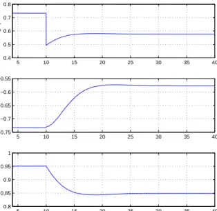
Figure 7.7 Dynamic responses in active and reactive power due to a step response

inV_ac∗. 85

Figure 7.8 Dynamic responses of the HVDC system due to a step response inV_ac∗. 86

Figure 7.9 V-I characteristics of the HVDC. 86

Figure 7.10 Dynamic responses of active power from synchronous generator, DFIG

and through HVDC due to a change in wind speed under different PI

controller settings. 87

Figure 7.11 Dynamic responses of the real power from the synchronous generator

(excluding the load), the wind farm and through the HVDC due to

wind speed changes. 88

Figure 7.12 Dynamic responses of the voltage controller and the turbine governor

due to wind speed changes. 89

Figure 7.13 Dynamic responses of the HVDC due to wind speed changes. 89

Figure 7.14 Dynamic responses of the DFIG wind farm due to wind speed changes. 90

Figure 7.15 Dynamic responses of the active power from synchronous generator,

load, DFIG and through HVDC due to load change. 91

Figure 7.16 Dynamic responses of the generator speed, firing angle, dc voltage and

Vac due to load change. 91

Figure 7.17 Dynamics of the inverter variables during A-L-G fault at the inverter

side. 92

Figure 7.18 Dynamics of the rectifier variables during A-L-G fault at the inverter

side. 93

Figure 8.1 P Q limit and operating points of the DFIG under different wind speeds. 97

Figure 8.2 Reactive power flow. 97

Figure 8.3 Simplified radial system. 98

Figure 8.5 Operation region of the ac bus voltage. 100

Figure 8.6 Dynamic responses of active power, reactive power, and apparent power

at the ac bus under wind speed changes whenVac= 0.87. 102

Figure 8.7 Dynamic responses of active power, reactive power, and apparent power

at the ac bus under wind speed changes whenVac= 0.993. 102

Figure 8.8 Dynamic responses of DFIG and HVDC variables, wind speed increases

from 9m/s to 10m/s at 10s, and increases from 10m/s to 11m/s at 25s,

when Vac = 0.993. 103

Figure 8.9 Dynamic responses of active power, reactive power, and apparent power

at the ac bus under wind speed changes whenVac= 0.98. 104

Figure 8.10 Dynamic responses of DFIG and HVDC variables, wind speed increases

from 9m/s to 10m/s at 10s, and increases from 10m/s to 11m/s at 25s,

ABSTRACT

As the most developed renewable energy source, wind energy attracts the most research attentions. Wind energy is easily captured far away from the places where wind energy is used. Because of this unique characteristic of the wind, the generation and delivery systems of the wind energy need to be well controlled. The objective of this dissertation work is modeling and control of wind generation and its High Voltage Direct-Current (HVDC) delivery system.

First of all, modeling of the Doubly-fed Induction Generator (DFIG)-based wind farm is presented including dynamic models of the wind turbine, shaft system and DFIG. Detailed models of the rectifier and inverter of HVDC are given as well. Furthermore, a control scheme for rotor-side converter (RSC) and grid-side converter (GSC) is studied. A control method for the HVDC delivery system is also presented.

Secondly, wind farms are prone to faults due to the remote locations. Unbalanced fault is the most frequent. Therefore, fault-ride through (FRT) of an ac connected DFIG-based wind farm is discussed in this dissertation. Dynamic responses of the wind farm under unbalanced grid conditions are analyzed including rotor current harmonics, torque pulsation and dc-link voltage ripples. Coordinated control strategy is proposed for DFIG under unbalanced fault.

Thirdly, when a wind farm is connected to remote ac grids through HVDC, active power balance between DFIG-based wind farm and HVDC delivery needs to be obtained. In other words, the power delivered through HVDC should balance the varying wind power extracted from the wind farm. Therefore, control methods of DFIG and HVDC are modi-fied. A coordinated control scheme is proposed to keep the power balance. The transmitted power through HVDC is regulated by adjusting the firing angle of the converter under

dif-ferent wind speeds. Both average and detailed models of the wind farm and HVDC delivery are built in Matlab/Simulink and Matlab/SimPowerSystems. Case studies validate the ef-fectiveness of the proposed control method.

Fourthly, the fast power routing capability of line-commutated converter (LCC)-HVDC is investigated when the wind energy is delivered through LCC-HVDC transmission. Such capability is most desired in future grids with high penetration of wind energy. The pro-posed technology replaces the traditional LCC-HVDC rectifier power order control by an ac voltage order control. This technology enables the HVDC rectifier ac bus to act as an infinite bus and absorb fluctuating wind power. A study system consisting of an ac system, an LCC-HVDC, and a doubly-fed induction generator (DFIG) based wind farm is built in Matlab/SimPowersystems. Simulation experiments are carried out to demonstrate the proposed HVDC rectifier control in routing fluctuating wind power and load change. Parameters of the proposed voltage order control are also investigated to show their impact on HVDC power routing and ac fault recovery.

Finally, for the wind farm with LCC-HVDC delivery, reactive power needs to be pro-vided for the HVDC. Hence, reactive power capability of the DFIG is discussed because DFIG is capable of providing reactive power to the LCC-HVDC. Since the reactive power is directly related to the voltage, the upper and lower limits of the rectifier ac bus voltage are investigated. Case studies are carried out in Matlab/Simulink to verify the system dynamics when the ac bus voltage is within and out of the limits.

CHAPTER 1 INTRODUCTION

1.1 Background

To date, the most electrical power is generated from fossil fuel. This causes adverse

environmental effects: global warming due toCO₂ emission. The environmental issues and

possible energy crisis contribute to the interest in clean and renewable energy resources such as solar, wind, tidal, etc. Among the various renewable energy resources, wind energy is the most attractive. By 2012, up to 12% of world’s electricity will be supplied by wind power [3]. In the United States, 40,180 MW of wind power had been installed across the country by December 31, 2010 [4]. The newest “20% Wind Energy by 2030” report, published by the U.S. Department of Energy in 2008, analyzes the feasibility of generating 20% of the nation’s electricity from wind power by 2030 [5].

With the high penetration of wind energy in power systems, suitable sites need to be found for wind generation plants. Studies [6, 7] show that offshore sites have higher and more stable potential wind capabilities compared with onshore ones. Furthermore, complaints from residents due to the aesthetics disruption and noise pollution are also factors that develop the offshore wind farms. Currently, the largest operational offshore wind farm in the world is Thanet in the United Kingdom, with capability of 300MW [8]. As for the United States, a report “A National Offshore Wind Strategy: Creating an Offshore Wind Energy Industry in the United States” was unveiled by the U.S Department of Energy on February 7, 2011. This plan will accelerate the development of offshore wind farm projects in the United States.

The current state-of-the-art wind generation technology is doubly-fed induction genera-tor (DFIG). A DFIG is an induction machine, with both the stagenera-tor and the rogenera-tor connected to electrical sources. The stator of a DFIG is directly connected to the grid, while the rotor is connected to the grid through back-to-back voltage source converters: rotor-side con-verter (RSC) and grid-side concon-verter (GSC). The two concon-verters are coupled with a dc-link capacitor. Compared with other wind turbine generator configuration, a DFIG-based wind farm offers noticeable advantages: it can achieve variable speed and constant frequency [9]. Wind farms are required to ride through abnormal grid voltage conditions [10]. Due to its asymmetric configuration, DFIGs suffer adverse impact due to grid unbalance [11, 12]. Unbalanced faults will cause unbalanced current, and torque pulsations [11]. Consequently, oscillations of the stator power will be produced. Moreover, ripples of the dc-link voltage will result in the power oscillations of the power of both RSC and GSC, which causes damage to the dc capacitor between RSC and GSC.

For DFIG-based large offshore wind farms, one key challenge is the transmission of bulk power over long distances. Two alternative transmission methods are available for connecting offshore wind farms to the grid: high-voltage alternating current (HVAC) and high-voltage direct current (HVDC) [13, 14]. Detailed comparison of ac and dc transmission is discussed in [15] considering the transmission costs, technical issues, and reliability. Compared with traditional HVAC, HVDC offers many advantages as follows [13, 16, 15].

1. Power flow is fully defined and controlled.

2. The frequencies of the ac systems at the sending and receiving ends are independent. 3. Cable power losses are lower.

4. Costs are lower for long distance bulk power transmission.

In the application of wind energy transmission, the main disadvantage of HVAC is that the load loss increases significantly with increasing wind farm capability and the distance to load. Generally, HVAC is suitable for medium wind farms with transmission distance less

than 100-150 km [13]. Alternatively, HVDC connection is more preferable for large wind farms with longer transmission lines.

There are two types of HVDC connection methods: voltage source converter (VSC)-HVDC using IGBTs and line-commutated converter (LCC)-(VSC)-HVDC using thyristors. Ref-erences [17, 18] addressed research in VSC-HVDC. VSC-HVDC is self-commutating, and it does not require an external voltage source. Reactive power can be independently con-trolled at each ac network, but its power rating is limited within 500MW. Furthermore, the main drawback of VSC-HVDC is the higher losses due to fast switching operations. On the other hand, LCC-HVDC can handle higher power capability compared with VSC-HVDC, and the power losses are lower. However, LCC-HVDC needs a strong grid to ensure normal commutation process. Reactive power absorption is another key issue because the current always lags behind the voltage due to delayed firing angle. Both LCC-HVDC and VSC-HVDC are studied in [13]. For wind farms with bulk power and long transmission distance, LCC-HVDC is preferable. Hence, this dissertation investigates the issues related with LCC-HVDC.

1.2 Problem Identification

This dissertation focuses on the control of wind generation and its HVDC delivery system. The following challenges are studied.

First, wind farms are often located in remote areas. Rural grids are weak and unstable, and prone to faults. National grid codes impose requirements on wind farms for fault-ride through (FRT) capability in order to prevent their disconnection during network faults. In practice, most faults in power system are unbalanced faults. Hence, control of wind farm under unbalanced grid conditions is studied in this dissertation.

Second, for wind energy with HVDC delivery system, active power balance is the key factor to ensure the normal operation of the system. In other words, the active power gen-erated by the wind farm should balance the power taken by LCC-HVDC, local loads and

losses. As the wind speed is ever-changing, the generated electrical power from DFIGs also fluctuates. The corresponding dc power output from the rectifier should follow the change of the electrical power from wind generation to achieve power balance. Any imbalance will cause stress on the wind turbine. Then large fluctuations will be observed in the rotor speed and electromagnetic torque. Therefore, active power balance needs to be studied in the DFIG-based wind generation system with LCC-HVDC connection. Normally, power order control is adopted in the rectifier of LCC-HVDC. However, the power order is always changing due to the fluctuating wind speeds. There will be some delay in the communi-cation links which send the remote power order signal. On the other hand, LCC-HVDC is fast in power routing. Therefore, the traditional power order control is not suitable here. The ac bus voltage order is selected to achieve the fast power routing capability of LCC-HVDC.

Third, a main drawback of the LCC-HVDC is reactive power consumption. For wind farms with LCC-HVDC delivery systems, reactive power must be provided for the HVDC converters to ensure normal operation since the voltage always lags behind the current. Usually, synchronous static compensator (STATCOM) is placed on the point of common coupling (PCC) to provide the reactive power demand of the LCC-HVDC. For variable speed DFIG-based wind farm with back-to-back pulse width modulation (PWM) convert-ers, both the stator and the GSC have the capability of providing reactive power. Hence, a STATCOM may not be necessary. However, when the wind speed increases, the capability to provide reactive power by a DFIG-based wind farm decreases. Meanwhile, there is an increase in reactive power loss in the transformer and ac lines. As a consequence, the reactive power transmitted to the LCC-HVDC could be reduced. Hence, coordination of the DFIG wind farm terminal voltage and HVDC rectifier voltage is necessary to make sure the required reactive power is supplied to the HVDC converters.

1.3 Tasks

The main tasks carried out in this dissertation are as follows:

Task 1 presents the modeling of DFIG-based wind farm and its HVDC delivery system. As for the wind farm, aerodynamic modeling of the wind turbine, dynamic modeling of the DFIG are presented. For the HVDC, detailed model of the converter and ac filters are given. Existing control schemes for RSC and GSC are discussed. Detailed PI controller design procedure is presented. Control parts of the HVDC are also described.

Task 2 studies the FRT of direct connected DFIG-based wind farm. Dynamics of the DFIG are analyzed under unbalanced grid conditions. A novel control technique is proposed for both RSC and GSC. Through simulation studies in Matlab/Simlink, the proposed control method shows higher performance compared with the existing dual-sequence control scheme.

Task 3 studies the active power balance between the wind farm and its HVDC delivery. Since the harvested wind power is always changing due to the varying wind speed, the delivered power through HVDC should be able to track the wind power to keep power balance. Coordinated control strategy of the wind farm and HVDC delivery is proposed for the rectifier of the HVDC. The firing angle of the thyristor is adjusted to change the power extracted from the wind farm, while the frequency and bus voltage is kept constant. Task 4 investigates the fast power routing capability of HVDC. LCC-HVDC is the power electronic device-based technology which is widely used in wind power transmission. It can route the power order from the wind farm very fast. The well-known power order control could be an obstacle in the power routing of HVDC, because of the delay in process of the power order computation and sending. Therefore, the ac bus voltage order is proposed to achieve the fast power routing capability of LCC-HVDC. The system dynamics are studied under wind speed change and the load change. Furthermore, the ac fault recovery capability of the system is also investigated with the proposed control strategy.

Task 5 analyzes the reactive power coordination of DFIG-based wind farm with LCC-HVDC delivery. Reactive power absorption is a key issue in the wind farm system with

LCC-HVDC delivery, since the voltage of each phasor lags behind the current. Besides the traditional ac filters, DFIG could also provide reactive power to HVDC. Hence, the active/reactive power limits of DFIG should be identified. In addition, the limiting range of the bus voltage is also investigated to ensure normal operation of the system under different wind speeds.

1.4 Approach

Both average and detailed models of the wind farm with its HVDC delivery are stud-ied in this dissertation. Matlab/Simlink and Matlab/SimPowerSystems are adopted for average and detailed models respectively.

Here, Simulink is an environment for time-domain simulation of dynamic systems. The blocks in the library offer advantages for control design. However, the dynamic models are average models based on math equations. All the variables are dc components as all

the ac variables in abc reference frame are transferred into qd reference frame.

There-fore, the high frequency components are ignored. For the DFIG-based wind farm with HVDC delivery, power electronic devices are the key components. Details of the converters cannot be presented in Simulink. Hence, Matlab/SimPowerSystems is also used. Mat-lab/SimPowerSystems is a toolbox developed by MathWorks especially for modeling and simulating electrical power systems. It provides most of the electrical components com-monly used in power systems, such as machines, electrical sources, power electronics, etc. In the distributed resource library, there are blocks for wind generation, which is a good resource for this research. Detailed models of DFIG-based wind farm with HVDC deliv-ery are more easily built in Matlab/SimPowerSystems. All the necessary components are addressed in the model, including transformers, ac filters, pulse generators. Furthermore, the dynamic responses of the detailed converters model are all captured. That is why Matlab/SimPowerSystems is adopted in this research work.

1.5 Outline of the Dissertation

The structure of the dissertation is organized as follows:

Chapter 1 gives a brief introduction of the studied issues including background infor-mation, problem identification, tasks, and approach adopted in this dissertation.

Chapter 2 presents a detailed literature survey on wind generators and their delivery systems. The development of wind turbines is reviewed, especially, DFIG-base wind tur-bine is described. Due to the rural location of wind farms, the FRT of an ac connected DFIG-based wind farm is also addressed. On the other hand, for the delivery system, the configurations of both VSC-HVDC and LCC-HVDC are presented. Also their advantages and disadvantages are compared in detail. Moreover, two key issues, active power balance and reactive power coordination, are investigated in the delivery system.

Chapter 3 studies the modeling of wind generator system and LCC-HVDC delivery including the the aerodynamic modeling of wind turbine, dynamic modeling of the DFIG, modeling of the converters and the ac filters in HVDC.

Chapter 4 discusses the control of wind generator system and LCC-HVDC delivery. Vector control is adopted in the DFIG control. For both the RSC and GSC, PI controllers are used for the outer and inner control loops. Hence, typical parameter design procedure of the PI controller is also given. Furthermore, control of the converters of HVDC is described.

Chapter 5 presents the FRT of DFIG-based wind farm under unbalanced grid condi-tions. When there is unbalanced fault on the grid, the root cause of the high frequency har-monics in rotor currents, the electromagnetic torque and the dc-link voltage are discussed. A simple control technique for limiting the harmonics of the dc-link voltage and the elec-tromagnetic torque is proposed. Simulation results for a 2MW DFIG in Matlab/Simulink confirms the effectiveness of the proposed control technique.

Chapter 6 studies the active power balance between DFIG-based wind farm and its

delivery system. Due to ever-changing characteristics of the wind, the captured wind

balance the ac power to obtain normal operation of the system. A coordination control scheme is proposed for the rectifier to adjust the firing angle at different wind speeds. Case studies in Matlab/Simlink and Matlab/SimPowerSystems are also given to show the effectiveness of the proposed control method.

Chapter 7 investigates the fast power routing capability of HVDC in wind energy trans-mission. Due to the intermittent characteristics of wind, the traditional power order control of the rectifier is not suitable. Voltage control is proposed for the rectifier, therefore the HVDC rectifier ac bus acts as an infinite bus. Simulation studies are carried out in Mat-lab/SimPowersystems to demonstrate the proposed control in routing fluctuating wind power and load change.

Chapter 8 presents the reactive power coordination between a DFIG-based wind farm and LCC-HVDC. To obtain reactive power coordination, first the DFIG should work within its operating limit while supplying reactive power for LCC-HVDC, a lower limit of the ac bus voltage is identified. In addition, as wind speed increases and in order to ensure reactive power provision from DFIG to LCC-HVDC, the ac bus voltage also has an upper limit. Case studies of an aggregated 200MW wind farm with LCC-HVDC connection is tested in Matlab/Simulink. Simulation results under different ac bus voltages verify the analysis.

Chapter 9 summarizes the main conclusions of this dissertation and provides some suggestions for the future work.

CHAPTER 2

LITERATURE SURVEY OF WIND GENERATORS AND DELIVERY SYSTEMS

2.1 Wind Energy Systems

Wind has become a prominent renewable energy supplier. The development of wind turbines is one of the key drivers. The dominate wind turbines are classified according to their ability of speed control as: fixed-speed wind turbine or variable speed wind turbine.

Wind turbines are built based on the “Danish concept” [9]: a fixed-speed wind turbine using squirrel-cage induction machine (SCIG) is directly connected to a three-phase power grid as shown in Fig. 2.1. The capacitor bank provides reactive power for the SCIG. The soft-starter is used for smoother grid connection. However, fixed-speed wind turbines have many disadvantages: first, the varying wind speed will cause fluctuations in mechanical power which is converted to fluctuating electrical power. Hence, sturdy mechanical design is required in case of wind gusts. Second, the reactive power cannot be controlled [19].

Figure 2.1. Fixed-speed wind generator topology.

There are three types of variable speed wind turbines configurations: limited variable speed using wound rotor induction generators as shown in Fig. 2.2, variable wind speed wind turbine using doubly-fed induction generators as shown in Fig. 2.3 and variable speed

wind turbine based on permanent magnet synchronous generators (PMSG) as shown in Fig. 2.4. The first type of configuration achieves limited variable speed control through the additional rotor resistance; the rotor resistance can be changed to control the slip and in turn the output power. DFIG-based configuration is widely used in current wind turbine systems. The back-to-back converters with partial rating are connected to the rotor circuit and the grid. Both active and reactive power could be controlled through the converters. Details of a DFIG will be introduced in Chapter 3. In the third type, PMSG is connected to a full-scale converter then to the grid. A gearbox may not be necessary in this kind of configuration. Instead, a direct driven generator with a larger diameter is used [20].

Figure 2.2. Limited variable speed wind turbine topology.

Figure 2.4. Variable wind generator topology with a full scale converter.

2.1.1 Doubly-Fed Induction Generator

Currently, DFIG-based wind generation as shown in Fig. 2.3 is the state-of-the-art wind generator technology [21, 22]. The stator windings of a DFIG are connected directly to the grid while the rotor windings are connected to back-to-back converters with 25%-30% of the generator rating. The stator provides active power to the grid. The power flow direction in the rotor depends on the operation condition. In sub-synchronous operation, the power is fed into the rotor; in super-synchronous operation, the power flows out of the rotor and fed to the grid through the converters. DFIGs offer many advantages [9, 23, 24] including variable speed operation, decoupled active power/reactive power control, maximum wind power capture, etc. Studies in [25, 26] focus on modeling of DFIG-based wind turbines and their impacts on the power systems. In [25], the power converters are modeled as controlled voltage sources to regulate the rotor currents. The model performance is verified in power system simulation tool PSS/E. [26] derives a dynamic model of a DFIG, which is suitable for transient stability study. Vector control is usually adopted for the converter control of DFIG. The active and reactive power could be controlled independently through the RSC. While the GSC keeps the dc-link voltage and supplies reactive power to the grid to keep the terminal voltage in desired range [21, 22, 27, 28].

2.1.2 Fault-Ride Through of an AC-Connected DFIG-Based Wind Farm

For wind farms in remote rural areas, the grid voltage is vulnerable to disturbances. Among the power system disturbances, asymmetric faults are more frequent than

sym-metric faults. To obtain continuous operation of the wind generation system, fault-ride through (FRT) capability needs to be studied during unbalanced grid voltage. Unbalanced grid conditions in DFIGs give rise to high frequency components in rotor currents and torque, which can cause excessive shaft stress and winding losses [29]. Existing control techniques in literature designed to minimize the torque pulsations include (i) RSC com-pensation by supplying negative sequence voltages to the rotor circuits [30, 31] to suppress the negative sequence components in the rotor currents and ripples in the electromagnetic torque, (ii) GSC compensation by compensating negative sequence currents to the grid [32] to keep the stator currents free of negative sequence components and thus eliminate the negative sequence components in the rotor currents.

Dual control schemes for both the RSC and GSC are proposed in [33, 10, 34, 12] to suppress the dc-link voltage ripples, pulsations in the rotor currents and electromagnetic torque. Negative sequence compensation has been adopted in the above mentioned ref-erences. Negative sequence compensation can be realized through current control loops [32, 35, 33, 10, 12] or through direct power control [36, 37]. The cascaded control structure with inner fast current control and outer slower power/voltage control is widely used in converter control and is also used in the commercial DFIG technology [38]. Hence, this control structure is widely adopted in the existing research.

2.2 Wind Energy Delivery Systems

2.2.1 Comparison of AC and DC Delivery

Electrical power could be transmitted through both ac and dc. DC is especially used for very long distance bulk power transmission. For wind energy transmission, dc is more attractive because of the following advantages compared with ac transmission [39]:

1. Lower losses

The ac resistance of a conductor is higher than dc resistance because of skin effect. Furthermore, there is reactive power consumption in ac transmission system.

There-fore, to transmit the same amount of real power, the power loss in ac lines is much higher than in dc lines.

2. Lower cost

Typical investment costs for an overhead line transmission with ac and dc is shown in Fig. 2.5 [1]. From Fig. 2.5, there is a break-even-distance at about 600-800 km [1]. For transmission lines above this value, ac cost is less than dc because of the high investment in terminal stations of dc. However, for transmission lines with a length above this level, the cost of dc will be less than ac. For undersea cables, the break-even-distance is much smaller, at about 50km [1]. For offshore wind farms using undersea cables, dc is a wise choice over ac.

Figure 2.5. Typical investment cost for an ac line and a dc line [1].

3. Better grid connection

Different areas of the world have different network frequencies. For example, Japan has both 50 Hz and 60 Hz networks. In North America, the power grid is divided into three unsynchronized parts. In such case, HVDC is suitable for connecting unsynchronized ac networks.

2.2.2 HVDC Technology

With the development of the wind energy industry, the majority of wind farms are built in rural areas around the world, requiring long transmission lines to the grid. HVDC delivery has been verified to be more attractive than ac transmission [40, 39] in the connec-tion of offshore wind farms. As introduced in Chapter 1, there are two HVDC connecconnec-tion types: VSC-HVDC using IGBTs, and LCC-HVDC using thyristors.

2.2.2.1 VSC-HVDC

The configuration of a VSC-HVDC consists of two VSC units and a dc-link as shown in Fig. 2.6. The dc capacitors at both ends of the dc line maintain a stable voltage at the converter ends. The current main three topologies for VSC transmission are two-level topology, multilevel diode-clamped topology, and multilevel floating-capacitor topology. They are compared in terms of cost, dc capacitor size and commutation inductance in [41]. An overview of VSC-HVDC is also presented in [42]. VSC-HVDC technology remains competitive in wind energy delivery due to its valuable advantages such as independent control of active and reactive power, no external voltage source for commutation, and fast dynamic response. When VSC-HVDC is used for DFIG-based wind farms, the wind farm side VSC collects the wind energy from the wind farm, while the grid side VSC transmits the collected energy to onshore grid. As an indication of power balance, the dc-voltage is kept constant through wind farm side VSC control [17]. VSCs are able to operate with weak ac grids through independent control of active and reactive power [40]. VSC-HVDC is more feasible for weak ac systems with short circuit ratio (SCR) less than 2.5 since commutation voltage is not needed. Hence, VSC-HVDC is suitable for connecting wind farms to weak ac grids [43]. Interconnection of two weak ac systems through VSC-HVDC is discussed in [44], where a novel power synchronization control is proposed.

The power rating of VSC-HVDC is restricted to about 500MW [13] due to the limit of IGBTs. For large wind energy delivery, VSC-HVDC is less competitive compared with

Figure 2.6. Configuration of a DFIG-based wind farm with VSC-HVDC delivery.

LCC-HVDC. On the other hand, the power loss of VSC-HVDC is higher due to the higher frequency switching used for PWM.

2.2.2.2 LCC-HVDC

A single-line schematic diagram of LCC-HVDC for wind farm transmission is illustrated in Fig. 2.7. It includes two valve groups, three-phase two-winding converter transformers, dc cables and ac filters at each end.

For LCC-HVDC, the line-commutated converters cause characteristic harmonic volt-ages and currents. Hence, ac filters are required at the two ends. The orders of these harmonics depends on the pulse number of the converter configuration. For p-pulse

con-verter, the generated voltage/current harmonics orders will be pk±1, where k is an integer.

For 12-pulse converter, the ac filters are designed typically for 11th and 13th harmonics. Usually, besides the single tuned filters, a high-pass filter branch is also included in the ac filters, and extra shunt capacitors are also needed to provide reactive power. Details of ac filter design for HVDC systems are introduced in [45]. [46] gives the parameters algo-rithm of ac filters in HVDC transmission systems. C-type filter is specifically presented in [47, 48].

Due to the firing angle and commutation angle of thyristors, the converter voltage in each phase always lags behind its current, hence reactive power supply needs to be guaranteed. Besides ac filters, static synchronous compensator (STATCOM) is another provider of reactive power. When LCC-HVDC is used to deliver wind energy from DFIG-based wind generation, reactive power compensation could also be provided by DFIG through flexible reactive power control of DFIG.

Despite the above mentioned drawbacks, LCC-HVDC is still the preferred option for bulk-power and long-distance dc transmission. First of all, the capability of LCC-HVDC is larger than VSC-HVDC. Secondly, the power loss is lower for long-distance delivery compared with VSC-HVDC.

Extensive literature has been published in research on LCC-HVDC applications in wind energy system. For DFIG-based wind generation systems with LCC-HVDC transmission, coordinated control of HVDC-link and DFIG has been proposed in [49]. Stator flux refer-ence value is provided for DFIG control, and the firing angle of the rectifier at the sending end of HVDC-link is used to regulate the frequency of the local ac system.

Figure 2.7. Configuration of a DFIG-based wind farm with LCC-HVDC delivery.

In [16, 14], LCC-HVDC system without STATCOM is studied for DFIG-based wind farm system connection. Grid frequency control is used to regulate the HVDC rectifier firing angle/dc-link current, and hence to control the power flow in the system.

Tradi-tionally, LCC-HVDC needs commutation voltage supplied by synchronous compensators. STATCOM is widely used to provide the commutation voltage instead of synchronous compensators because of its lower cost. STATCOM issues in offshore wind farm with LCC-HVDC connection are discussed in [50] in details. With STATCOM, the offshore could be controlled as an infinite source to obtain higher system dynamics. Recently, hy-brid HVDC system was proposed by [51]. The hyhy-brid system consists of a thyristor-based rectifier, and a STATCOM with PWM inverter.

2.3 Active Power Balance between Wind Farm and HVDC Delivery System

When a wind farm is connected to a grid through LCC-HVDC, the generated electrical power from the wind farm must balance the active power taken by LCC-HVDC and the dissipation. Any imbalance will cause voltage/frequency variations of the local ac grid[49]. The transmitted power of the HVDC should be able to track the varying power due to different wind speeds. Frequency control is proposed in [49] to adjust the firing angle of the rectifier of HVDC transmission without STATCOM. If the wind speed increases, the decreased firing angle will cause the dc current to increase. Thus more power is delivered through HVDC to keep the power balance.

For the LCC-HVDC transmission system with STATCOM converter, any power imbal-ance will accumulate on the dc capacitor of the STATCOM, causing the dc-link voltage to fluctuate [50]. Hence, the dc voltage of STATOM could be considered as the indication of power imbalance, which is used to change the dc current order of HVDC converter [13]. Once the dc voltage of STATCOM is kept constant, power balance could be achieved.

2.4 Reactive Power Coordination of Wind Farm with LCC-HVDC Delivery

Newly-established grid codes require wind turbines to have reactive power capabil-ity to support grid voltage [52]. On the other hand, as mentioned in the above section, LCC-HVDC needs reactive power because the voltage lags the current in each phase. The general reactive power source for LCC-HVDC is a capacitor bank and STATCOM. When

a DFIG-based wind farm is connected to LCC-HVDC, the stator of DFIG could also pro-vide reactive power to LCC-HVDC, since DFIG can achieve independent active/reactive power control through rotor excitation current. Furthermore, the GSC could also produce reactive power under weak grid conditions. Hence, the reactive power capability of DFIG needs to be investigated considering the DFIG-based wind farm with LCC-HVDC connec-tion. If the reactive power supply from DFIG and shunt capacitor satisfy the LCC-HVDC requirements, STATCOM may not be necessary, thus the cost could be greatly reduced.

The reactive power capability of the wind turbine depends on grid connection type. For DFIG-based wind turbine, the total power fed into the grid is supplied from the stator and GSC. [52, 53, 54] have done some research on the reactive power capability of DFIG. Considering the stator current, rotor current and rotor voltage limits, the actual active and reactive power capability limits could be obtained. [53] concludes that the main factor in limiting the reactive power production is the rotor current; Additional limiting factors such as system losses, speed variation, and filter are considered in [54] to get a more accurate reactive power capability. For the offshore wind farm with HVDC connection[55], the total DFIG-based wind turbine capability limits are obtained considering stator current limit, rotor current limit and steady-state stability limit. Taking into account the total capability limits and steady-state stability limits, the maximum reactive power limit depends on rectifier voltage and the generated active power while the minimum reactive power lies on the rectifier voltage.

2.5 Other Related Study on Wind Farm with HVDC Delivery

Small signal analysis is a useful method for power system analysis, it provides valuable information about the dynamic characteristics for controller design [2]. Some work based on small signal analysis has been done in wind farms with HVDC systems. Dynamic analysis of the rectifier subsystem is presented in [51]. Through the eigenvalue analysis method, the ac current dynamic of the rectifier is investigated and double loop control scheme is designed. [56] also applies small signal analysis to an offshore wind farm with

line-commutated HVDC link. Eigenvalue analysis is performed to design a PID rectifier-current regulator, which is also verified in improving damping of the offshore wind farm.

CHAPTER 3

MODELING OF WIND GENERATION SYSTEM AND LCC-HVDC DELIVERY

This chapter gives the modeling details of the wind energy generation system with LCC-HVDC delivery. The topology of the studied system is shown in Fig. 3.1. Modeling of each part will be introduced in subsequent sections of this chapter.

Figure 3.1. System topology.

3.1 DFIG-Based Wind Turbine

3.1.1 Aerodynamic Modeling of Wind Turbine

The wind turbine is an important mechanical device in the wind power generation system. The total wind power swept by the rotor blade of the wind turbine can be expressed as: Pwind = ρ 2πR 2_V3 ω (3.1)

where ρ is the air density, R is the rotor radius of wind turbine, and Vω is wind speed.

is impossible to exact all the kinetic energy of the wind. This refers to a term: power

coefficient defined as Cp. Hence, the mechanical power is given by:

Pm=CpPwind (3.2)

The power coefficient Cp is a nonlinear function of the blade pitch angleθ, and the tip

speed ratioλas:

Cp = (0.44−0.0167θ)sin(

π(λ−3)

15−0.3θ)−0.00184(λ−3)θ (3.3)

where the tip speed ratioλis:

λ= ωmR

Vω

(3.4)

where ωm is the mechanical angular velocity. For the old simple wind turbine, the blade

pitch angle is constant. With a fixed pitch angle θ, the relationship between power

coef-ficient Cp and tip speed ratio λis similar as the curve shown in Fig. 3.2. At the optimal

pointλopt, maximum power coefficientCpis achieved. Assuming a constant wind speedVω,

the tip speed ratioλ is proportional to mechanical angular velocity ωm. Thus, the curves

ofCp againstωmare in the similar shape as shown in Fig. 3.2 under different wind speeds

but their optimal operation points are different. In the case of variable-speed wind turbine,

the maximum power coefficient Cp is achieved through adjusting the rotational speed of

the wind turbine. Thereby, the maximum output mechanical power point is reached. When the wind speed is above rated speed, which means the wind power exceeds the generator rating, pitch angle control is considered a common way to regulate the aerodynamic torque. In such condition, the mechanical power is reduced to the rating (1 pu) through adjusting the pitch angle. When the wind speed is less than the rated speed, the pitch angle is adjusted to the minimum value to get the maximum mechanical power. In both cases, the pitch angle controller senses the speed change to regulate the output power. A typical structure of pitch angle controller is shown in Fig. 3.3. The pitch angle

λ

C

opt

λ

Figure 3.2. Power coefficient curve.

is determined by the input variables: rotor speed, generator power. The actual rotor speed is compared with its reference value, and the error is sent to the PI controller to get the reference value of the pitch angle. On the other hand, the error of the generator power signal is also input into the PI controller to generate the reference pitch angle.

* r ω r

ω

Figure 3.3. Wind turbine pitch angle controller.

The two-mass shaft model is proved sufficient for the stability analysis of DFIG-based wind generation in [57]. The schematic representation of a two-mass shaft is depicted in Fig. 3.4. The two-mass shaft model is described by the following equations:

dωt dt = − Dt+Dtg 2Ht ωt+ Dtg 2Ht ωr− 1 2Ht Ttg+ Tm 2Ht (3.5) dωr dt = Dtg 2Hg ωt− Dt+Dtg 2Hg ωr+ 1 2Hg Ttg+ Te 2Hg (3.6) dTtg dt = Ktgω0ωt−Ktgω0ωr (3.7)

where Dt and Dg are the damping coefficients of the turbine and generator, Dtg is the

damping coefficient of the flexible coupling between the two masses, Ht and Hg are the

inertia constants for the turbine and the generator, Ktg is the shaft stiffness.

t

ω

ω

Figure 3.4. Schematic diagram of the shaft.

3.1.2 Dynamic Modeling of the DFIG

The dynamic of the DFIG is expressed through a series differential equations in sta-tionary abc reference frame. All the variables of the equations such as voltage, current, and flux linkage are time-varying variables, which make the computation process complex. In the late 1920s, R. H. Park introduced an approach to reduce the complexity of electrical machine analysis: Park’s transformation [58]. In the Park’s transformation, the stator vari-ables are transferred to a reference frame rotating at the synchronous speed. The detailed transformation is expressed as:

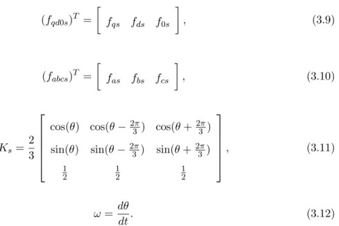
where (fqd0s)T = fqs fds f0s , (3.9) (fabcs)T = fas fbs fcs , (3.10) Ks= 2 3 ⎡ ⎢ ⎢ ⎢ ⎢ ⎣

cos(θ) cos(θ−2₃π) cos(θ+ 2₃π)

sin(θ) sin(θ−2₃π) sin(θ+2₃π)

1 2 12 12 ⎤ ⎥ ⎥ ⎥ ⎥ ⎦, (3.11) ω= dθ dt. (3.12)

In the above equations,f could either be voltage, current or flux linkage. The relationship

between theabcstationary reference frame and qd rotating reference frame can be seen in

Fig. 3.5. Fig. 3.6 shows the equivalent circuit of DFIG in qd reference frame. The stator

e

ω

e θ

Figure 3.5. Reference frame relationship.

s v

v

Figure 3.6. The equivalent circuit of DFIG.

⎡ ⎢ ⎢ ⎢ ⎢ ⎢ ⎢ ⎢ ⎢ ⎢ ⎢ ⎢ ⎢ ⎢ ⎢ ⎣ vqs vds v₀s v_qr v_dr v_0r ⎤ ⎥ ⎥ ⎥ ⎥ ⎥ ⎥ ⎥ ⎥ ⎥ ⎥ ⎥ ⎥ ⎥ ⎥ ⎦ = ⎡ ⎢ ⎢ ⎢ ⎢ ⎢ ⎢ ⎢ ⎢ ⎢ ⎢ ⎢ ⎢ ⎢ ⎢ ⎣ rs 0 0 0 0 0 0 rs 0 0 0 0 0 0 rs 0 0 0 0 0 0 r_r 0 0 0 0 0 0 r_r 0 0 0 0 0 0 r_r ⎤ ⎥ ⎥ ⎥ ⎥ ⎥ ⎥ ⎥ ⎥ ⎥ ⎥ ⎥ ⎥ ⎥ ⎥ ⎦ ⎡ ⎢ ⎢ ⎢ ⎢ ⎢ ⎢ ⎢ ⎢ ⎢ ⎢ ⎢ ⎢ ⎢ ⎢ ⎣ iqs ids i₀s i_qr i_dr i_0r ⎤ ⎥ ⎥ ⎥ ⎥ ⎥ ⎥ ⎥ ⎥ ⎥ ⎥ ⎥ ⎥ ⎥ ⎥ ⎦ + ⎡ ⎢ ⎢ ⎢ ⎢ ⎢ ⎢ ⎢ ⎢ ⎢ ⎢ ⎢ ⎢ ⎢ ⎢ ⎣ 0 ω 0 0 0 0 −ω 0 0 0 0 0 0 0 0 0 0 0 0 0 0 0 ω−ωr 0 0 0 0 ω−ωr 0 0 0 0 0 0 0 0 ⎤ ⎥ ⎥ ⎥ ⎥ ⎥ ⎥ ⎥ ⎥ ⎥ ⎥ ⎥ ⎥ ⎥ ⎥ ⎦ ⎡ ⎢ ⎢ ⎢ ⎢ ⎢ ⎢ ⎢ ⎢ ⎢ ⎢ ⎢ ⎢ ⎢ ⎢ ⎣ λqs λds λ₀s λ_qr λ_dr λ_0r ⎤ ⎥ ⎥ ⎥ ⎥ ⎥ ⎥ ⎥ ⎥ ⎥ ⎥ ⎥ ⎥ ⎥ ⎥ ⎦ + ⎡ ⎢ ⎢ ⎢ ⎢ ⎢ ⎢ ⎢ ⎢ ⎢ ⎢ ⎢ ⎢ ⎢ ⎢ ⎣ ˙ λqs ˙ λds ˙ λ₀s ˙ λ_qr ˙ λ_dr ˙ λ_0r ⎤ ⎥ ⎥ ⎥ ⎥ ⎥ ⎥ ⎥ ⎥ ⎥ ⎥ ⎥ ⎥ ⎥ ⎥ ⎦ (3.13)

where vqs, vds are the q-axis and d-axis stator voltages, vqr, vdr are the q-axis and d-axis

rotor voltages, rs is the stator resistance, r

r is the rotor resistance, Lls is the stator self

inductance,L_lr is the rotor self inductance, M is the mutual inductive reactance,ω is the

are expressed as: ⎡ ⎢ ⎢ ⎢ ⎢ ⎢ ⎢ ⎢ ⎢ ⎢ ⎢ ⎢ ⎢ ⎢ ⎢ ⎣ λqs λds λ₀s λ_qr λ_dr λ_0r ⎤ ⎥ ⎥ ⎥ ⎥ ⎥ ⎥ ⎥ ⎥ ⎥ ⎥ ⎥ ⎥ ⎥ ⎥ ⎦ = ⎡ ⎢ ⎢ ⎢ ⎢ ⎢ ⎢ ⎢ ⎢ ⎢ ⎢ ⎢ ⎢ ⎢ ⎢ ⎣ Lls+M 0 0 M 0 0 0 Lls+M 0 0 M 0 0 0 Lls 0 0 0 M 0 0 L_lr+M 0 0 0 M 0 0 L_lr+M 0 0 0 0 0 0 L_lr ⎤ ⎥ ⎥ ⎥ ⎥ ⎥ ⎥ ⎥ ⎥ ⎥ ⎥ ⎥ ⎥ ⎥ ⎥ ⎦ ⎡ ⎢ ⎢ ⎢ ⎢ ⎢ ⎢ ⎢ ⎢ ⎢ ⎢ ⎢ ⎢ ⎢ ⎢ ⎣ iqs ids i₀s i_qr i_dr i_0r ⎤ ⎥ ⎥ ⎥ ⎥ ⎥ ⎥ ⎥ ⎥ ⎥ ⎥ ⎥ ⎥ ⎥ ⎥ ⎦ (3.14)

In addition, the electromagnetic torque can be described as:

Te=

2 3

p

2(λdsiqs−λqsids) (3.15)

where p is the number of poles.

The stator active power fed into the grid can be calculated through the following equa-tion:

Ps=vqsiqs+vdsids (3.16)

While the reactive power that the stator absorbs or feeds into the grid is calculated:

Qs=vqsids−vdsiqs (3.17)

For GSC, the equivalent circuit in qd reference frame can be obtained from Fig. 3.7,

and the grid side voltage is shown as follows:

vg =vs−ωsLtg

dig

dt −jωsLtgig (3.18)

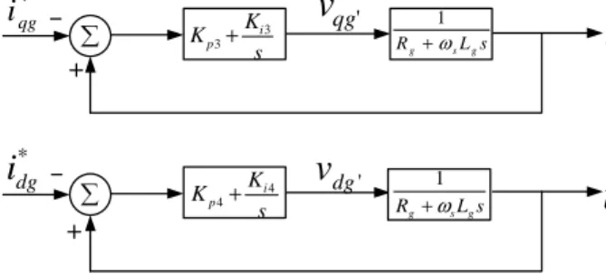
The voltage and current relationship in qd-axis can be written as:

vqg =vqs−ωsLtg

diqg

s

v

v

i

ω

Figure 3.7. The equivalent circuit of GSC.

vdg=vds−ωsLtg

didg

dt +ωsLtgiqg (3.20)

The dynamics of the dc-link between RSC and GSC can be expressed as follows:

CVdc

dVdc

dt =Pg−Pr=

1

2(vqgiqg+vdgidg−(vqriqr+vdridr)) (3.21)

wherePg is the active power of the GSC,Pr is the active power of the RSC.

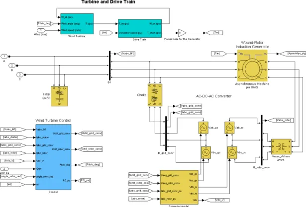
The model of DFIG-based wind farm in Matlab/SimPowerSystems is shown in Fig. 3.8. The dynamics of the wind turbine and drive train are considered. Pitch angle control is also

given. Since inqd reference frame, the variables are dc signals and hence easier to control.

Consequently, all the variables in abc reference frame are transformed into qd reference

frame. Vector control is adopted for the RSC and GSC, and the required synchronization angle is derived through phasor-locked loop (PLL).

3.2 LCC-HVDC

3.2.1 Rectifier

A typical rectifier model in Matlab/SimPowerSystems is shown in Fig. 3.9. The recti-fier is a three-phase, full-wave bridge circuit as shown in Fig. 3.10. The cathodes of valves 1, 3 and 5 are connected together. For the upper row, the valve with the most positive phase-to-neutral voltage conducts. For the lower row, the anodes of valves 2, 4 and 6 are connected together. Therefore, the valve with the most negative phase-to-neutral voltage

conducts. The waveforms of the voltage are illustrated in Fig. 3.11. When ωtis between

00 and 600, van is the highest positive phase, vbn is the lowest negative phase. Hence,

valve 1 of the upper row and valve 6 of the lower row conduct. For the next 600, valve

1 and 2 conduct. Then valve 3 and 2 conduct. From the analysis, it is easy to find that

each valve conducts for 1200. The instantaneous direct voltage is composed of several 600

segments. Therefore, the average direct voltage Vd0 can be calculated by the integration

of the instantaneous dc voltage over any 600 period as follows:

Vd0 = 3 π ₆₀0 0 vabd(ωt) = 3 π ₆₀0 0 √ 2Vacsin(ωt+ 600)d(ωt) = 3 √ 6 π Vac

whereVac is the rms line-to-neutral voltage. Vd0 is the “ideal no-load direct voltage.”

Figure 3.9. Schematic diagram of the rectifier in Matlab/SimPowerSystems.

A simplified rectifier equivalent circuit is shown in Fig. 3.12. For a monopole, 12-pulse rectifier of HVDC-link, considering the firing angle delay and commutation angle, the re-lationship between the dc and ac voltage is [2]:

a

i

i

i

v

v

v

Figure 3.10. Three-phase full-wave bridge rectifier.

an

v

v

v

v

ω

ω

whereRrec= _π3Xc is the commutating reactance per phase,Vdr and Idc are the dc voltage

and dc current,α is the firing delay angle of the rectifier and is in the range of 00−900.

dr

V

R

α

cos

V

Figure 3.12. The equivalent circuit of the rectifier.

The power relationship is expressed as:

Pdc=VdrIdc=Pac (3.23)

Qac =Pactan(θ) (3.24)

where Pdc is the dc power,Pac and Qac are the active and reactive power, θ is the power

factor.

3.2.2 Inverter

The inverter operation is similar to the rectifier, the only difference is that the firing

angle is in the range of 900 and 1800. Normally β, called the ignition advance angle, is

used to describe inverter performance. An inverter model in Matlab/SimPowerSystems is shown in Fig. 3.13 and its equivalent circuit is shown in Fig. 3.14.

The relationship between the ac and dc quantities are as follows:

⎧ ⎪ ⎪ ⎨ ⎪ ⎪ ⎩ Vdi=Vd0cosβ+RinvIdc Vd0 = _π3 √ 2BT Vac(L−L) (3.25)

Figure 3.13. Schematic diagram of the inverter in Matlab/SimPowerSystems. dc

I

V

cos

β

V

R

whereβ is the firing advance angle of the inverter in the range of 900 and 1800;Rinv = _π3Xc

is the commutating reactance per phase, B is the number of bridges in series, T is the

transformer ration, and VacL−L is the line-to-line rms value of the ac voltage.

Ignore the power losses, then the ac power is equal to the dc power:

Pac =Pdc (3.26)

3.2.3 AC Filters

LCC converters generate low order harmonic currents and harmonic voltages, which will be injected into power system. The harmonic orders depend on the pulse number.

A converter with p pulse generates harmonic orders pq±1, q is an integer. For 12-pulse

converter, the ac harmonic orders will be 12q ±1 (i.e., 11th, 13th, 23th, 25th...). Also,

their amplitudes decrease with harmonic order. Some undesirable effects may occur if the harmonics enter the ac power system, such as telephone interference, overheating of capacitors and generators, higher losses, etc.[59, 60, 61]. Normally, filters are adopted on the ac side to reduce the harmonics. Furthermore, they can also supply reactive power at the fundamental frequency. A typical filter system contains single tuned filter, high-pass filter and C-type filter.

3.2.3.1 Single Tuned Filter

A single tuned filter is a kind of band-pass filter tuned at a single frequency. Fig. 3.15 shows a block diagram of the single tuned filter. The values of the capacitor, inductance and resistance are determined by the tuned frequency, reactive power at nominal voltage

and quality factor [45, 46]. The reactive powerQcat fundamental frequencyf1is calculated

as follows: Qc = n

2

n2−1 V2

Xc, where n is the harmonic order, V is the nominal line-line voltage,

Xc is the capacitor reactance at fundamental frequency. Then the value of the capacitor

is: C= Qc(n2−1)

Figure 3.15. Single tuned filter.

Figure 3.16. High-pass

fil-ter. Figure 3.17. C-type filter.

The quality factor Q is a measurement of the tuning frequency. Q is the quality factor

of the reactance at the tuning frequency: Q= nXL

R =

Xc

nR. Then the value of the resistance

is: R= _ωCnQ1 . In addition, the value of the inductance is: L= _ω2n1_2C.

A Double tuned filter is also used in the ac filters for HVDC, which is a kind of single tuned filter. The only difference is that the double tuned filter tuned at two different harmonic orders.

3.2.3.2 High-Pass Filter

The high-pass filter is used to filter out the high frequency harmonics. As seen in Fig. 3.16, the resistance R and inductance L are connected in parallel. The quality factor of the high-pass filter is the quality factor of the parallel RL circuit at the tuning frequency:

Q= R

L·2πfn

where fn is the tuning frequency. The values of capacitor, inductance and resistance can be calculated as follows [45]: ⎧ ⎪ ⎪ ⎪ ⎪ ⎪ ⎪ ⎨ ⎪ ⎪ ⎪ ⎪ ⎪ ⎪ ⎩ C = Qc(n2−1) ωn2V2 L= _(n2−V₁₎2_ωQ c R=Q·2πLfn (3.28) 3.2.3.3 C-Type Filter

A C-type filter is a kind of high-pass filter as shown in Fig. 3.17, where the inductance L is replaced with a series LC circuit. It is capable not only of filtering out low order harmonics, but also of providing reactive power. The quality factor of a C-type filter is the same as the high-pass filter:

Q= R

L·2πfn

(3.29)

R, L values can be calculated in the same way as high-pass filter [47, 48].

⎧ ⎪ ⎪ ⎨ ⎪ ⎪ ⎩ L= _(n2−V₁₎2_ωQ c R=Q·2πLfn (3.30)

The only difference is the capacitors. C₁ is determined by the required reactive power at

the nominal voltage, which is derived as follows:

C₁ = Qc

ωV2 (3.31)

The series of C₁ and C₂ is an equivalent C, which could be found as follows:

⎧ ⎪ ⎪ ⎨ ⎪ ⎪ ⎩ C= Qc(n2−1) ωn2V2 1 C = C1₁ + C1₂ (3.32)

3.2.3.4 Example

This paragraph gives an example to explain the function of the ac filters and their parameter design for a real system. For the thyristor-based HVDC link given in the demo of Matlab/SimPowerSystems, it is a 1000MW HVDC system used to transmit power from a 500KV, 60Hz system to a 345KV, 50Hz system. For a rated 1000MW LCC-HVDC, the required reactive power at the ac side is about 50%-60% of the dc power under most normal operations [62]. For the sending end, an ac filter block composed of a capacitor bank, single tuned filter and high-pass filter is designed to give 600 MVar reactive power. The capacitor bank provides 150MVar. The parameters of a single tuned filter to filter out the 11th filter is designed as follows:

The capacitor value is:

C = Qc(n

2₋₁₎

ωn2V2 =

150∗106(112−1)

2π∗60∗112(500∗103)2 ≈1.6μF (3.33)

where this single tuned filter provides 150Mvar reactive power, hence, Qc = 150∗106. It

aims to filter out the 11th filter, then n= 11. The frequency of the ac side is 60Hz, which

meansω = 2π60, and V is the rated ac voltage. Then the capacitor needed for the single

tuned filter is about 1.6μF.

The quality factor Q of the filter is set as 100. Then the parameters of the resistance and inductance can be calculated as:

⎧ ⎪ ⎪ ⎨ ⎪ ⎪ ⎩ R= _ωCnQ1 = _{2π60∗1.6∗10}1_{(−6)∗11∗100} ≈1.5Ω L= _ω2n1_2C = _(2π60)21121_{∗1.6∗10−6} ≈36mH (3.34)

A single tuned filter to filter out the 13th harmonic and high-pass filter tuned to the 24th harmonic could also be designed in a similar way.