Research
iCity & Big Data—Review
Strategies and Principles of Distributed Machine Learning on Big Data
Eric P. Xing
*
, Qirong Ho, Pengtao Xie, Dai Wei
School of Computer Science, Carnegie Mellon University, Pittsburgh, PA 15213, USAa r t i c l e i n f o a b s t r a c t
Article history:
Received 29 December 2015 Revised 1 May 2016 Accepted 23 May 2016 Available online 30 June 2016
The rise of big data has led to new demands for machine learning (ML) systems to learn complex mod-els, with millions to billions of parameters, that promise adequate capacity to digest massive datasets and offer powerful predictive analytics (such as high-dimensional latent features, intermediate repre-sentations, and decision functions) thereupon. In order to run ML algorithms at such scales, on a distrib-uted cluster with tens to thousands of machines, it is often the case that significant engineering efforts are required—and one might fairly ask whether such engineering truly falls within the domain of ML research. Taking the view that “big” ML systems can benefit greatly from ML-rooted statistical and algo-rithmic insights—and that ML researchers should therefore not shy away from such systems design—we discuss a series of principles and strategies distilled from our recent efforts on industrial-scale ML solu-tions. These principles and strategies span a continuum from application, to engineering, and to theo-retical research and development of big ML systems and architectures, with the goal of understanding how to make them efficient, generally applicable, and supported with convergence and scaling guaran-tees. They concern four key questions that traditionally receive little attention in ML research: How can an ML program be distributed over a cluster? How can ML computation be bridged with inter-machine communication? How can such communication be performed? What should be communicated between machines? By exposing underlying statistical and algorithmic characteristics unique to ML programs but not typically seen in traditional computer programs, and by dissecting successful cases to reveal how we have harnessed these principles to design and develop both high-performance distributed ML software as well as general-purpose ML frameworks, we present opportunities for ML researchers and practitioners to further shape and enlarge the area that lies between ML and systems. .
© 2016 THE AUTHORS. Published by Elsevier LTD on behalf of Chinese Academy of Engineering and Higher Education Press Limited Company. This is an open access article under the CC BY-NC-ND license (http://creativecommons.org/licenses/by-nc-nd/4.0/). Keywords:
Machine learning
Artificial intelligence big data Big model Distributed systems Principles Theory Data-parallelism Model-parallelism * Corresponding author.
E-mail address: [email protected] http://dx.doi.org/10.1016/J.ENG.2016.02.008
2095-8099/© 2016 THE AUTHORS. Published by Elsevier LTD on behalf of Chinese Academy of Engineering and Higher Education Press Limited Company. This is an open access article under the CC BY-NC-ND license (http://creativecommons.org/licenses/by-nc-nd/4.0/).
Contents lists available at ScienceDirect
j o u r n a l h o m e p a g e : w w w. e l s e v i e r. c o m / l o c a t e / e n g
Engineering
1. Introduction
Machine learning (ML) has become a primary mechanism for dis-tilling structured information and knowledge from raw data, turning them into automatic predictions and actionable hypotheses for di-verse applications, such as: analyzing social networks [1]; reasoning about customer behaviors [2]; interpreting texts, images, and vide-os [3]; identifying disease and treatment paths [4]; driving vehicles without the need for a human [5]; and tracking anomalous activity for cybersecurity [6], among others. The majority of ML applications are supported by a moderate number of families of well-developed
ML approaches, each of which embodies a continuum of technical elements from model design, to algorithmic innovation, and even to perfection of the software implementation, and which attracts ever-growing novel contributions from the research and develop-ment community. Modern examples of such approaches include graphical models [7–9], regularized Bayesian models [10–12], nonparametric Bayesian models [13,14], sparse structured mod-els [15,16], large-margin methods [17,18], deep learning [19,20], matrix factorization [21,22], sparse coding [23,24], and latent space modeling [1,25]. A common ML practice that ensures mathemati-cal soundness and outcome reproducibility is for practitioners and
researchers to write an ML program (using any generic high-level programming language) for an application-specific instance of a particular ML approach (e.g., semantic interpretation of images via a deep learning model such as a convolution neural network). Ideally, this program is expected to execute quickly and accurately on a vari-ety of hardware and cloud infrastructure: laptops, server machines, graphics processing units (GPUs), cloud computing and virtual machines, distributed network storage, Ethernet and Infiniband net-working, to name just a few. Thus, the program is hardware-agnos-tic but ML-explicit (i.e., following the same mathemahardware-agnos-tical principle when trained on data and attaining the same result regardless of hardware choices).
With the advancements in sensory, digital storage, and Internet communication technologies, conventional ML research and devel-opment—which excel in model, algorithm, and theory innovations— are now challenged by the growing prevalence of big data collec-tions, such as hundreds of hours of video uploaded to video-sharing sites every minute†, or petabytes of social media on billion-plus-user social networks‡. The rise of big data is also being accompanied by an increasing appetite for higher-dimensional and more complex ML models with billions to trillions of parameters, in order to sup-port the ever-increasing complexity of data, or to obtain still higher predictive accuracy (e.g., for better customer service and medical di-agnosis) and support more intelligent tasks (e.g., driverless vehicles and semantic interpretation of video data) [26,27]. Training such big ML models over such big data is beyond the storage and computa-tion capabilities of a single machine. This gap has inspired a growing body of recent work on distributed ML, where ML programs are executed across research clusters, data centers, and cloud provid-ers with tens to thousands of machines. Given P machines instead of one machine, one would expect a nearly P-fold speedup in the time taken by a distributed ML program to complete, in the sense of attaining a mathematically equivalent or comparable solution to that produced by a single machine; yet, the reported speedup often falls far below this mark. For example, even recent state-of-the-art implementations of topic models [28] (a popular method for text analysis) cannot achieve 2× speedup with 4× machines, because of mathematical incorrectness in the implementation (as shown in Ref.
[25]), while deep learning on MapReduce-like systems such as Spark has yet to achieve 5× speedup with 10× machines [29]. Solving this scalability challenge is therefore a major goal of distributed ML re-search, in order to reduce the capital and operational cost of running big ML applications.
Given the iterative-convergent nature of most—if not all—major ML algorithms powering contemporary large-scale applications, at a first glance one might naturally identify two possible avenues to-ward scalability: faster convergence as measured by iteration num-ber (also known as convergence rate in the ML community), and faster per-iteration time as measured by the actual speed at which the system executes an iteration (also known as throughput in the system community). Indeed, a major current focus by many distrib-uted ML researchers is on algorithmic correctness as well as faster convergence rates over a wide spectrum of ML approaches [30,31]
However, it is difficult for many of the “accelerated” algorithms from this line of research to reach industry-grade implementations because of their idealized assumptions on the system—for example, the assumption that networks are infinitely fast (i.e., zero synchro-nization cost), or the assumption that all machines make the algo-rithm progress at the same rate (implying no background tasks and only a single user of the cluster, which are unrealistic expectations
for real-world research and production clusters shared by many us-ers). On the other hand, systems researchers focus on high iteration throughput (more iterations per second) and fault-recovery guar-antees, but may choose to assume that the ML algorithm will work correctly under non-ideal execution models (such as fully asyn-chronous execution), or that it can be rewritten easily under a given abstraction (such as MapReduce or Vertex Programming) [32–34]. In both ML and systems research, issues from the other side can be-come oversimplified, which may in turn obscure new opportunities to reduce the capital cost of distributed ML. In this paper, we pro-pose a strategy that combines ML-centric and system-centric think-ing, and in which the nuances of both ML algorithms (mathematical properties) and systems hardware (physical properties) are brought together to allow insights and designs from both ends to work in concert and amplify each other.
Many of the existing general-purpose big data software plat-forms present a unique tradeoff among correctness, speed of execu-tion, and ease-of-programmability for ML applications. For example, dataflow systems such as Hadoop and Spark [34] are built on a MapReduce-like abstraction [32] and provide an easy-to-use pro-gramming interface, but have paid less attention to ML properties such as error tolerance, fine-grained scheduling of computation, and communication to speed up ML programs. As a result, they of-fer correct ML program execution and easy programming, but are slower than ML-specialized platforms [35,36]. This (relative) lack of speed can be partly attributed to the bulk synchronous parallel (BSP) synchronization model used in Hadoop and Spark, in which machines assigned to a group of tasks must wait at a barrier for the slowest machine to finish, before proceeding with the next group of tasks (e.g., all Mappers must finish before the Reducers can start) [37]. Other examples include graph-centric platforms such as GraphLab and Pregel, which rely on a graph-based “vertex program-ming” abstraction that opens up new opportunities for ML program partitioning, computation scheduling, and flexible consistency con-trol; hence, they are usually correct and fast for ML. However, ML programs are not usually conceived as vertex programs (instead, they are mathematically formulated as iterative-convergent fixed-point equations), and it requires non-trivial effort to rewrite them as such. In a few cases, the graph abstraction may lead to incorrect execution or suboptimal execution speed [38,39]. Of recent note is the parameter server paradigm [28,36,37,40,41], which pro-vides a “design template” or philosophy for writing distributed ML programs from the ground up, but which is not a programmable platform or work-partitioning system in the same sense as Hadoop, Spark, GraphLab, and Pregel. Taking into account the common ML practice of writing ML programs for application-specific instances, a usable software platform for ML practitioners could instead offer two utilities: ① a ready-to-run set of ML workhorse implemen-tations—such as stochastic proximal descent algorithms [42,43], coordinate descent algorithms [44], or Markov Chain Monte Carlo (MCMC) algorithms [45]—that can be re-used across different ML al-gorithm families; and ② an ML distributed cluster operating system supporting these workhorse implementations, which partitions and executes these workhorses across a wide variety of hardware. Such a software platform not only realizes the capital cost reductions obtained through distributed ML research, but even complements them by reducing the human cost (scientist- and engineer-hours) of big ML applications, through easier-to-use programming libraries and cluster management interfaces.
With the growing need to enable data-driven knowledge
distil-† https://www.youtube.com/yt/press/statistics.html
lation, decision making, and perpetual learning—which are repre-sentative hallmarks of the vision for machine intelligence—in the coming years, the major form of computing workloads on big data is likely to undergo a rapid shift from database-style operations for deterministic storage, indexing, and queries, to ML-style operations such as probabilistic inference, constrained optimization, and ge-ometric transformation. To best fulfill these computing tasks, which must perform a large number of passes over the data and solve a high-dimensional mathematical program, there is a need to revisit the principles and strategies in traditional system architectures, and explore new designs that optimally balance correctness, speed, programmability, and deployability. A key insight necessary for guiding such explorations is an understanding that ML programs are optimization-centric, and frequently admit iterative-convergent algorithmic solutions rather than one-step or closed form solutions. Furthermore, ML programs are characterized by three properties:
① error tolerance, which makes ML programs robust against limited errors in intermediate calculations; ② dynamic structural depend-encies, where the changing correlations between model parameters must be accounted for in order to achieve efficient, near-linear par-allel speedup; and ③ non-uniform convergence, where each of the billions (or trillions) of ML parameters can converge at vastly differ-ent iteration numbers (typically, some parameters will converge in 2–3 iterations, while others take hundreds). These properties can be contrasted with traditional programs (such as sorting and database queries), which are transaction-centric and are only guaranteed to execute correctly if every step is performed with atomic correct-ness [32,34]. In this paper, we will derive unique design principles for distributed ML systems based on these properties; these design principles strike a more effective balance between ML correctness, speed, and programmability (while remaining generally applicable to almost all ML programs), and are organized into four upcoming sections: ① How to distribute ML programs; ② how to bridge ML computation and communication; ③ how to communicate; and
④ what to communicate. Before delving into the principles, let us first review some necessary background information about itera-tive-convergent ML algorithms.
2. Background: Iterative-convergent machine learning (ML) algorithms
With a few exceptions, almost all ML programs can be viewed as optimization-centric programs that adhere to a general mathematical form: max
(
,)
A L x A or minA L(
x, A)
, where(
,)
(
{
,}
1;)
( )
N i i i A =f x y = A r A+L
x (1)In essence, an ML program tries to fit N data samples (which may be labeled or unlabeled, depending on the real-world application being considered), represented by
{
,}
N1i i i x y =
x (where yi is present only for labeled data samples), to a model represented by A. This fitting is performed by optimizing (maximizing or minimizing) an overall objective function L, composed of two parts: a loss function, f, that describes how data should fit the model, and a structure-induc-ing function, r, that incorporates domain-specific knowledge about the intended application, by placing constraints or penalties on the values that A can take.
The apparent simplicity of Eq. (1) belies the potentially complex structure of the functions f and r, and the potentially massive size
of the data x and model A. Furthermore, ML algorithm families are often identified by their unique characteristics on f, r, x, and A. For example, a typical deep learning model for image classification, such as Ref. [20], will contain tens of millions through billions of matrix-shaped model parameters in A, while the loss function f ex-hibits a deep recursive structure f
( )
=f f f1(
2(
3( )
+)
+)
thatlearns a hierarchical representation of images similar to the human visual cortex. Structured sparse regression models [4] for identifying genetic disease markers may use overlapping structure-inducing functions r
( )
=r A1( )
a +r A2( )
b +r A3( )
c +, where Aa, Ab, and Ac are overlapping subsets of A, in order to respect the intricate process of chromosomal recombination. Graphical models, particularly topic models, are routinely deployed on billions of documents x—that is, N ≥ 109, a volume that is easily generated by social media such as Facebook and Twitter—and can involve up to trillions of parameters θ in order to capture rich semantic concepts over so much data [26].Apart from specifying Eq. (1), one must also find the model parameters A that optimize L. This is accomplished by selecting one out of a small set of algorithmic techniques, such as stochastic gradient descent [42], coordinate descent [44], MCMC†[45], and variational inference (to name just a few). The chosen algorithmic technique is applied to Eq. (1) to generate a set of iterative-conver-gent equations, which are implemented as program code by ML practitioners, and repeated until a convergence or stopping criterion is reached (or, just as often, until a fixed computational budget is ex-ceeded). Iterative-convergent equations have the following general form:
A
( )
t =F(
A(
t−1 ,)
L(
A(
t−1 ,)
x)
)
(2)where, the parentheses (t) denotes iteration number. This general form produces the next iteration’s model parameters A(t), from the previous iteration’s A(t − 1) and the data x, using two functions:
① an update function ∆L (which increases the objective L) that
per-forms computation on data x and previous model state A(t − 1), and outputs intermediate results; and ② an aggregation function F that then combines these intermediate results to form A(t). For simplicity of notation, we will henceforth omit L from the subscript of ∆—with the implicit understanding that all ML programs considered in this paper bear an explicit loss function L (as opposed to heuristics or procedures lacking such a loss function).
Let us now look at two concrete examples of Eqs. (1) and (2), which will prove useful for understanding the unique properties of ML programs. In particular, we will pay special attention to the four key components of any ML program: ① data x and model A; ② loss function f(x, A); ③ structure-inducing function r(A); and ④ algo-rithmic techniques that can be used for the program.
Lasso regression. Lasso regression [46] is perhaps the simplest exemplar from the structured sparse regression ML algorithm fam-ily, and is used to predict a response variable yi given vector-valued features xi (i.e., regression, which uses labeled data)—but under the assumption that only a few dimensions or features in xi are inform-ative about yi. As input, Lasso is given N training pairs x of the form
(
,)
mi yi
x , i = 1,…, n, where the features are m-dimensional vec-tors. The goal is to find a linear function, parametrized by the weight vector A, such that ①A xT i yi, and ② the m-dimensional parame-ters A are sparse‡ (most elements are zero):
(
)
Lasso minAL
x, A, where(
)
(
)
{ }(
1)
( ) 2 T Lasso 1 1 , ; 1 , 2 N i i i n m i i n j i j r f y y λ a = = = =∑
− +∑
A x A A A x L x (3)† Strictly speaking, MCMC algorithms do not perform the optimization in Eq. (1) directly—rather, they generate samples from the function L, and additional procedures are applied to these samples to find a optimizer A*.
‡ Sparsity has two benefits: It automatically controls the complexity of the model (i.e., if the data requires fewer parameters, then the ML algorithm will adjust as required), and improves human interpretation by focusing the ML practitioner’s attention on just a few parameters.
or more succinctly in matrix notation: min1 22 1 2 − +λn A XA y A (4) where, T
[
]
1, , n m n× = ∈ X x x ;(
)
T 1, , n n y y = ∈ y ; 2 is the Euclide-an norm on Rn; 1 is the l1 norm on R m; and λn is some constant that balances model fit (the f term) and sparsity (the g term). Many algo-rithmic techniques can be applied to this problem, such as stochas-tic proximal gradient descent or coordinate descent. We will present the coordinate descent† iterative-convergent equation:
j
( )
Tj Tj k k(
1 ,)
n k j t ⋅ ⋅ ⋅ t λ ≠ = −∑
− A X y X X A (5)where,
(
Aj, : signλ)
=( )
Aj(
Aj −λ)
+ is the “soft-thresholding opera-tor,” and we assume the data is normalized so that for all j, T 1j j
⋅ ⋅ =
X X . Tying this back to the general iterative-convergent update form, we have the following explicit forms for Δ and F:
(
)
(
)
(
)
(
)
(
)
(
)
(
)
(
)
T T 1 1 1 Lasso T T 1 Lasso 1 1 , 1 , 1 , , k k k m k m m k k n m n t t t F t λ λ ⋅ ≠ ⋅ ⋅ ⋅ ≠ ⋅ ⋅ − − ∆ − = − − − =∑
∑
X y X X A A X y X X A u A u u x (6)where, uj= ∆ Lasso
(
A(
t−1 ,)
x)
j is the j-th element of ∆Lasso(
A(
t−1 ,)
x)
.Latent Dirichlet allocation topic model. Latent Dirichlet alloca-tion (LDA) [47] is a member of the graphical models ML algorithm family, and is also known as a “topic model” for its ability to identify commonly-recurring topics within a large corpus of text documents. As input, LDA is given N unlabeled documents x=
{ }
xi iN=1, where each document xi contains Ni words (referred to as “tokens” in the LDA literature) represented by xi = xi1, , , , xij xiNi . Each token{
1, ,}
ij
x ∈ V is an integer representing one word out of a vocabulary of V words—for example, the phrase “machine learning algorithm” might be represented as xi= x x xi1, ,i2 i3 = 25,60,13 (the correspond-ence between words and integers is arbitrary, and has no bearing on the accuracy of the LDA algorithm).
The goal is to find a set of parameters
{{ }
{ } { } }
1 11, , N N K ij i i i k k z = = = = A δ B
—“token topic indicators” zij∈
{
1, ,K}
for each token in eachdocu-ment, “document-topic vectors” δi∈Simplex
( )
K for each document,and K “word-topic vectors” (or simply, “topics”) Bk∈Simplex
( )
V —that maximizes the following log-likelihood‡ equation:
(
)
LDA maxA L x,A , where(
)
(
(
)
(
)
)
{ }(
)
(
)
(
)
( ) 1LDA cate. cate.
Dirichlet Dirichlet 1 1 1 1 ; , ln ln ln ln i ij N i i N N N K ij z ij i i k i j i k r f x z α β = = = = = = + + +
∑∑
∑
∑
A x A A B δ δ B L x (7) where, cate.( )
∏
u u v v ll l is the categorical (a.k.a., discrete)
proba-bility distribution;
( )
1 Dirichletα−
∏
v v
l l is the Dirichlet probability distribution; and α and β are constants that balance model fit (the f term) with the practitioner’s prior domain knowledge about the document-topic vectors δi and the topics Bk (the r term). Similar to Lasso, many algorithmic techniques such as Gibbs sampling and var-iational inference (to name just two) can be used on the LDA model; we will consider the collapsed Gibbs sampling equations††:
( )
(
)
(
)
(
)
(
)
old new old new , , , , , , 1 1, 1 1, 1 1, 1 1, ij ij k w k w i k i k i j t t t t ∀ − − = − + = − − = − + = B B δ δ (8)(
)
( )
(
(
) (
)
)
old new where 1 , 1 , 1 ij ij ij ij i k z t k z t ~ z x t t = − = δ − B −where, += and −= are the self-increment and self-decrement op-erators (i.e., δ, B, and z are being modified in-place); ~ P( ) means “to sample from distribution P,” and
(
z xij ij,δi(
t−1 ,) (
B t−1)
)
is the conditional probability‡‡ of zij given the current values of
(
1)
i t−
δ and B
(
t−1)
. The update ∆LDA(
A(
t−1 ,)
x)
proceeds in two stages: ① execute Eq. (8) over all document tokens xij; and ② out-put( )
{
{
(
1)
}
N1,{
(
1)
}
N1,{
(
1)
}
K1}
ij i i i k k
t = z t− = t− = t− =
A δ B . The aggregation
FLDA(A(t- 1), …) turns out to simply be the identity function.
2.1. Unique properties of ML programs
To speed up the execution of large-scale ML programs over a distributed cluster, we wish to understand their properties, with an eye toward how they can inform the design of distributed ML sys-tems. It is helpful to first understand what an ML program is “not”: Let us consider a traditional, non-ML program, such as sorting on MapReduce. This algorithm begins by distributing the elements to be sorted, x1,…, xN , randomly across a pool of M mappers. The Mappers hash each element xi into a key-value pair (h(xi), xi), where h is an “order-preserving” hash function that satisfies h(x) > h(y) if x > y. Next, for every unique key a, the MapReduce system sends all key-value pairs (a, x) to a Reducer labeled “a.” Each Reducer then runs a sequential sorting algorithm on its received values x and, finally, the Reducers take turns (in ascending key order) to output their sorted values.
The first thing to note about MapReduce sort, is that it is single- pass and non-iterative—only a single Map and a single Reduce step are required. This stands in contrast to ML programs, which are iter-ative-convergent and repeat Eq. (2) many times. More importantly, MapReduce sort is operation-centric and deterministic, and does not tolerate errors in individual operations. For example, if some Map-pers were to output a mis-hashed pair (a, x) where a ≠h(x) (for the sake of argument, let us say this is due to improper recovery from a power failure), then the final output will be mis-sorted because x will be output in the wrong position. It is for this reason that Hadoop and Spark (which are systems that support MapReduce) provide strong operational correctness guarantees via robust fault-tolerant systems. These fault-tolerant systems certainly require additional engineering effort, and impose additional running time overheads in the form of hard-disk-based checkpoints and lineage trees [34,49]— yet they are necessary for operation-centric programs, which may fail to execute correctly in their absence.
This leads us to the first property of ML programs: error toler-ance. Unlike the MapReduce sort example, ML programs are usually robust against minor errors in intermediate calculations. In Eq. (2), even if a limited number of updates ΔL are incorrectly computed or
transmitted, the ML program is still mathematically guaranteed to converge to an optimal set of model parameters A*—that is, the ML algorithm terminates with a correct output (even though it might take more iterations to do so) [37,40]. An good example is stochastic
† More specifically, we are presenting the form known as “block coordinate descent,” which is one of many possible forms of coordinate descent.
‡ A log-likelihood is the natural logarithm of a probability distribution. As a member of the graphical models ML algorithm family, LDA specifies a probability distribution, and hence has an associated log-likelihood.
†† Note that collapsed Gibbs sampling re-represents δ
i and Bk as integer-valued vectors instead of simplex vectors. Details can be found in Ref. [48].
‡‡ There are a number of efficient ways to compute this probability. In the interest of keeping this article focused, we refer the reader to Ref. [48] for an appropriate introduction.
gradient descent (SGD), a frequently used algorithmic workhorse for many ML programs, ranging from deep learning to matrix fac-torization and logistic regression [50–52]. When executing an ML program that uses SGD, even if a small random vector ε is added to the model after every iteration, that is, A(t) = A(t) + ε, convergence is still assured; intuitively, this is because SGD always computes the correct direction of the optimum A* for the update ΔL, so moving
A(t) around simply results in the direction being re-computed to suit [37,40]. This property has important implications for distrib-uted system design, as the system no longer needs to guarantee perfect execution, inter-machine communication, or recovery from failure (which requires substantial engineering and running time overheads). It is often cheaper to do these approximately, especially when resources are constrained or limited (e.g., limited inter-ma-chine network bandwidth) [37,40].
In spite of error tolerance, ML programs can in fact be more difficult to execute than operation-centric programs, because of de-pendency structure that is not immediately obvious from a cursory look at the objective L or update functions ΔL and F. It is certainly
the case that dependency structures occur in operation-centric programs: In MapReduce sort, the Reducers must wait for the Map-pers to finish, or else the sort will be incorrect. In order to see what makes ML dependency structures unique, let us consider the Lasso regression example in Eq. (3). At first glance, the ΔLasso update Eq. (6) may look like they can be executed in parallel, but this is only par-tially true. A more careful inspection reveals that, for the j-th model parameter Aj, its update depends on k ≠ jXT·jX·kAk (t – 1). In other words, potentially every other parameter Ak is a possible depend-ency, and therefore the order in which the model parameters Aare updated has an impact on the ML program’s progress or even cor-rectness [39]. Even more, there is an additional nuance not present in operation-centric programs: The Lasso parameter dependencies are not binary (i.e., are not only “on” or “off”), but can be soft-valued and influenced by both the ML program state and input data. Notice that if XT
·jX·k= 0 (meaning that data column j is uncorrelated with column k), then Aj and Ak have zero dependency on each other, and can be updated safely in parallel [39]. Similarly, even if XT·jX·k> 0, as long as Ak = 0, then Aj does not depend on Ak. Such dependency structures are not limited to one ML program; careful inspection of the LDA topic model update Eq. (8) reveals that the Gibbs sampler update for xij (word token j in document i) depends on ① all other word tokens in document i, and ② all other word tokens b in other documents a that represent the exact same word, that is, xij = xab[25]. If these ML program dependency structures are not respected, the result is either sub-ideal scaling with additional machines (e.g., < 2× speedup with 4× as many machines) [25] or even outright program failure that overwhelms the intrinsic error tolerance of ML pro-grams [39].
A third property of ML programs is non-uniform convergence, the observation that not all model parameters Aj will converge to their optimal values Aj* in the same number of iterations—a prop-erty that is absent from single-pass algorithms such as MapReduce sort. In the Lasso example in Eq. (3), the r(A) term encourages model parameters Aj to be exactly zero, and it has been empirical-ly observed that once a parameter reaches zero during algorithm execution, it is unlikely to revert to a non-zero value [39]. To put it another way, parameters that reach zero are already converged (with high, though not 100%, probability). This suggests that computation may be better prioritized toward parameters that are still non-zero, by executing ΔLasso more frequently on them—and such a strategy indeed reduces the time taken by the ML program to finish [39].
Similar non-uniform convergence has been observed and exploited in PageRank, another iterative-convergent algorithm [53].
Finally, it is worth noting that a subset of ML programs exhibit compact updates, in that the updates ΔLasso are, upon careful inspec-tion, significantly smaller than the size of the matrix parameters, |A|. In both Lasso (Eq. (3)) and LDA topic models [47], the updates ΔLasso generally touch just a small number of model parameters, due to sparse structure in the data. Another salient example is that of “matrix-parametrized” models, where A is a matrix (such as in deep learning [54]), yet individual updates ΔLasso can be decomposed into a few small vectors (a so-called “low-rank” update). Such compact-ness can dramatically reduce storage, computation, and communi-cation costs if the distributed ML system is designed with it in mind, resulting in order-of-magnitude speedups [55,56].
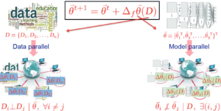
2.2. On data and model parallelism
For ML applications involving terabytes of data, using complex ML programs with up to trillions of model parameters, execution on a single desktop or laptop often takes days or weeks [20]. This computational bottleneck has spurred the development of many distributed systems for parallel execution of ML programs over a cluster [33–36]. ML programs are parallelized by subdividing the updates ΔL over either the data x or the model A—referred to
respec-tively as data parallelism and model parallelism.
It is crucial to note that the two types of parallelism are comple-mentary and asymmetric—complecomple-mentary, in that simultaneous data and model parallelism is possible (and even necessary, in some cases), and asymmetric, in that data parallelism can be applied ge-nerically to any ML program with an independent and identically distributed (i.i.d.) assumption over the data samples x1,…, xN. Such i.i.d. ML programs (from deep learning, to logistic regression, to top-ic modeling and many others) make up the bulk of practtop-ical ML us-age, and are easily recognized by a summation over data indices i in the objective L (e.g., Lasso Eq. (3)). Consequently, when a workhorse algorithmic technique (e.g., SGD) is applied to L, the derived update equations ΔL will also have a summation† over i, which can be easily
parallelized over multiple machines, particularly when the number of data samples N is in the millions or billions. In contrast, model parallelism requires special care, because model parameters Aj do not always enjoy this convenient i.i.d. assumption (Fig. 1)—therefore, which parameters Aj are updated in parallel, as well as the order in which the updates ΔL happen, can lead to a variety of outcomes:
from near-ideal P-fold speedup with P machines, to no additional speedups with additional machines, or even to complete program
Fig. 1. The difference between data and model parallelism: Data samples are always conditionally independent given the model, but there are some model parameters that are not independent of each other.
† For Lasso coordinate descent ΔLasso (Eq. (5)), the summation over i is in the inner product T 1
N j k i ij ik ⋅ ⋅ =
∑
=failure. The dependency structures discussed for Lasso (Section 2.1) are a good example of the non-i.i.d. nature of model parameters. Let us now discuss the general mathematical forms of data and model parallelism, respectively.
Data parallelism. In data parallel ML execution, the data
x = {x1,…,xN} is partitioned and assigned to parallel computational workers or machines (indexed by p = 1,…, P); we will denote the p-th data partition by xp. If the update function ΔL has an
outer-most summation over data samples i (as seen in ML programs with the commonplace i.i.d. assumption on data), we can split ΔL over
data subsets and obtain a data parallel update equation, in which ΔL(A(t – 1), xp) is executed on the p-th parallel worker:
A
( )
t =F(
A(
t−1 ,)
∑
pP=1∆L(
A(
t−1 ,)
xp)
)
(9) It is worth noting that the summation∑
Pp=1is the basis for a host of established techniques for speeding up data parallel execution, such as minibatches and bounded-asynchronous execution [37,40]. As a concrete example, we can write the Lasso block coordinate de-scent Eq. (6) in a data parallel form, by applying a bit of algebra:(
)
(
)
(
(
)
)
(
)
(
)
(
)
(
)
(
(
(
)
)
)
(
)
(
)
(
)
1 1 1 Lasso Lasso 1 1 Lasso Lasso 1 1 1 , 1 1 , , 1 , 1 , , p p i i i ik k i k p im i im ik k i k m P p n p P p n p m y t t y t t F t t λ λ ∈ ≠ ∈ ≠ = = − − ∆ − = − − ∆ − − = ∆ − ∑
∑
∑
∑
∑
∑
X X X A A X X X A A A u A x x x x x (10)where,
∑
i∈xp means (with a bit of notation abuse) to sum over all data indices i included in xp.Model parallelism. In model parallel ML execution, the model A is partitioned and assigned to workers/machines p = 1,…, P, and updated therein by running parallel update functions ΔL. Unlike
data parallelism, each update function ΔL also takes a scheduling
or selection function Sp,( t− 1), which restricts ΔL to operate on a
subset of the model parameters A(one basic use is to prevent dif-ferent workers from trying to update the same parameters):
( )
(
)
{
(
(
)
,( )1(
(
)
)
)
}
11 , 1 , p t 1 Pp
t =F t− ∆ t− S − t− =
A A L A A (11)
where, we have omitted the data x since it is not being partitioned over. Sp,( t− 1) outputs a set of indices {j1, j2,…}, so that ΔL only performs
updates on Aj1, Aj2,...; we refer to such selection of model parameters
as scheduling. The model parameters Aj are not, in general, independ-ent of each other, and it has been established that model parallel al-gorithms are effective only when each iteration of parallel updates is restricted to a subset of mutually independent (or weakly correlated) parameters [39,57–59], which can be performed by Sp,(t− 1).
The Lasso block coordinate descent updates (Eq. (6)) can be eas-ily written in a simple model parallel form. Here, Sp,(t− 1) chooses the same fixed set of parameters for worker p on every iteration, which we refer to by jp1,..., jpmp: ( ) ( )
(
( ))
(
)
( ) ( ) ( )(
)
( ) ( )(
( ))
(
)
(
)
( ) ( )(
( ))
(
)
( ) ( )(
( ))
(
)
1 1 1 1 T T Lasso , 1 T T Lasso 1, 1 1 Lasso 1, 1 Lasso Lasso , 1 1 1 , 1 1 1 , 1 , 1 , 1 , 1 , 1 , 1 p p p pmp pmp pmp j k j j k k p t j k j j k k n t n t m P t t t S t t t S t t S t F t t S t λ λ ⋅ ≠ ⋅ ⋅ − ⋅ ≠ ⋅ ⋅ − − − − − ∆ − − = − − ∆ − − ∆ − − − = ∆ − − ∑
∑
X y X X A A A X y X X A A A A A A A A (
)
( ) ( )(
( ))
(
)
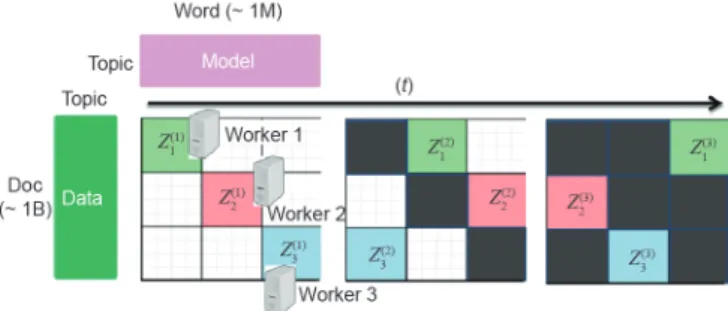
1 Lasso , 1 , 1 , 1 , P n n P t m t S t λ λ − ∆ − − A A (12)On a closing note, simultaneous data and model parallelism is also possible, by partitioning the space of data samples and model parameters (xi, Aj) into disjoint blocks. The LDA topic model Gibbs sampling equations (Eq. (8)) can be partitioned in such a block-wise manner (Fig. 2), in order to achieve near-perfect speedup with P machines [25].
3. Principles of ML system design
The unique properties of ML programs, when coupled with the complementary strategies of data and model parallelism, interact to produce a complex space of design considerations that goes beyond the ideal mathematical view suggested by the general iterative-convergent update equation, Eq. (2). In this ideal view, one hopes that the Δ and F functions simply need to be implemented equation-by-equation (e.g., following the Lasso regression data and model parallel equations given earlier), and then executed by a general-purpose distributed system—for example, if we chose a MapReduce abstraction, one could write Δ as Map and F as Reduce, and then use a system such as Hadoop or Spark to execute them. The reality, however, is that the highest-performing ML implemen-tations are not built in such a naive manner; and, furthermore, they tend to be found in ML-specialized systems rather than on gener-al-purpose MapReduce systems [26,31,35,36]. The reason is that high-performance ML goes far beyond an idealized MapReduce-like view, and involves numerous considerations that are not immedi-ately obvious from the mathematical equations: considerations such as what data batch size to use for data parallelism, how to partition the model for model parallelism, when to synchronize model views between workers, step size selection for gradient based algorithms, and even the order in which to perform Δ updates.
The space of ML performance considerations can be intimidating even to veteran practitioners, and it is our view that a systems in-terface for parallel ML is needed, both to ① facilitate the organized, scientific study of ML considerations, and also to ② organize these considerations into a series of high-level principles for developing new distributed ML systems. As a first step toward organizing these principles, we will divide them according to four high-level ques-tions: If an ML program’s equations (Eq. (2)) tell the system “what to compute,” then the system must consider: ① How to distribute the computation; ② How to bridge computation with inter-machine communication; ③ How to communicate between machines; and ④ What to communicate. By systematically addressing the ML con-siderations that fall under each question, we show that it is possible to build sub-systems whose benefits complement and accrue with each other, and which can be assembled into a full distributed ML system that enjoys orders-of-magnitude speedups in ML program execution time.
Fig. 2. High-level illustration of simultaneous data and model parallelism in LDA top-ic modeling. In this example, the three parallel workers operate on data/model blocks
Z1(1), Z2(1), and Z3(1) during iteration 1, then move on to blocks Z1(2), Z2(2), and Z3(2) during iteration 2, and so forth.
3.1. How to distribute: Scheduling and balancing workloads
In order to parallelize an ML program, we must first determine how best to partition it into multiple tasks—that is, we must parti-tion the monolithic Δ in Eq. (2) into a set of parallel tasks, following the data parallel form (Eq. (9)) or the model parallel form (Eq. (11))— or even a more sophisticated hybrid of both forms. Then, we must schedule and balance those tasks for execution on a limited pool of P workers or machines: That is, we ① decide which tasks go to-gether in parallel (and just as importantly, which tasks should not be executed in parallel); ② decide the order in which tasks will be executed; and ③ simultaneously ensure that each machine’s share of the workload is well-balanced.
These three decisions have been carefully studied in the con-text of operation-centric programs (such as the MapReduce sort example), giving rise (for example) to the scheduler system used in Hadoop and Spark [34]. Such operation-centric scheduler systems may come up with a different execution plan—the combination of decisions ① to ③—depending on the cluster configuration, existing workload, or even machine failure; yet, crucially, they ensure that the outcome of the operation-centric program is perfectly consistent and reproducible every time. However, for ML iterative-convergent programs, the goal is not perfectly reproducible execution, but rath-er convrath-ergence of the model parametrath-ers A to an optimum of the ob-jective function L (i.e., A approaches to within some small distance ε
of an optimum A*). Accordingly, we would like to develop a schedul-ing strategy whose execution plans allow ML programs to provably terminate with the same quality of convergence every time—we will refer to this as “correct execution” for ML programs. Such a strategy can then be implemented as a scheduling system, which creates ML program execution plans that are distinct from operation-centric ones.
Dependency structures in ML programs. In order to generate
a correct execution plan for ML programs, it is necessary to un-derstand how ML programs have internal dependencies, and how breaking or violating these dependencies through naive paralleliza-tion will slow down convergence. Unlike operaparalleliza-tion-centric programs such as sorting, ML programs are error-tolerant, and can automati-cally recover from a limited number of dependency violations—but too many violations will increase the number of iterations required for convergence, and cause the parallel ML program to experience suboptimal, less-than-P-fold speedup with P machines.
Let us understand these dependencies through the Lasso and LDA topic model example programs. In the model parallel version of Lasso (Eq. (12)), each parallel worker p {1,…, P} performs one or more ΔLasso calculations of the form XT·jy –
k ≠ jXT·jX·kAk (t – 1), which will then be used to update Aj. Observe that this calculation depends on all other parameters Ak, k ≠j through the term XT
·jX·kAk (t – 1), with the magnitude of the dependency being proportional to ① the correlation between the j-th and k-th data dimensions, XT·jX·k; and ② the current value of parameter Ak (t – 1). In the worst case, both the correlation XT·jX·k and Ak (t – 1) could be large, and therefore up-dating Aj, Ak sequentially (i.e., over two different iterations t, t + 1) will lead to a different result from updating them in parallel (i.e., at the same time in iteration t). Ref. [57] noted that, if the correlation is large, then the parallel update will take more iterations to converge than the sequential update. It intuitively follows that we should not “waste” computation trying to update highly correlated parameters in parallel; rather, we should seek to schedule uncorrelated groups of parameters for parallel updates, while performing updates for correlated parameters sequentially [39].
For LDA topic modeling, let us recall the ΔLDA updates (Eq. (8)): For every word token wij (in position j in document i), the LDA Gibbs sampler updates four elements of the model parametersB, δ (which are part of A): Bkold,wij(t – 1) – =1, Bknew,wij(t – 1) + =1, δi,kold(t – 1) – =1, and
δi,knew(t – 1) + =1, where kold = zij (t – 1) and knew = zij (t – 1) ~ P(zij |xij, δi(t – 1),
B(t – 1)). These equations give rise to many dependencies between different word tokens wij and wuv. One obvious dependency occurs when wij = wuv, leading to a chance that they will update the same elements of B (which happens when kold or knew are the same for both tokens). Furthermore, there are more complex dependencies inside the conditional probability P(zij |xij, δi(t – 1), B(t – 1)); in the interest of keeping this article at a suitably high level, we will summarize by noting that elements in the columns of, that is, B·,v, are mutually dependent, while elements in the rows of δ, that is, δi,·, are also mu-tually dependent. Due to these intricate dependencies, high-perfor-mance parallelism of LDA topic modeling requires a simultaneous data and model parallel strategy (Fig. 2), where word tokens wij must be carefully grouped by both their value v = wij and their document i, which avoids violating the column/row dependencies in B and
δ[25].
Scheduling in ML programs. In light of these dependencies, how can we schedule the updates Δ in a manner that avoids violating as many dependency structures as possible (noting that we do not have to avoid all dependencies thanks to ML error tolerance)—yet, at the same time, does not leave any of the P worker machines idle due to lack of tasks or poor load balance? These two considerations have distinct yet complementary effects on ML program execution time: Avoiding dependency violations prevents the progress per iteration of the ML program from degrading compared to sequential execu-tion (i.e., the program will not need more iteraexecu-tions to converge), while keeping worker machines fully occupied with useful compu-tation ensures that the iteration throughput (iterations executed per second) from P machines is as close to P times that of a single machine. In short, near-perfect P-fold ML speedup results from combining near-ideal progress per iteration (equal to sequential execution) with near-ideal iteration throughput (P times sequen-tial execution). Thus, we would like to have an ideal ML scheduling strategy that attains these two goals.
To explain how ideal scheduling can be realized, we return to our running Lasso and LDA examples. In Lasso, the degree to which two parameters Aj and Ak are interdependent is influenced by the data correlation XT·jX·k between the j-th and k-th feature dimensions—we refer to this and other similar operations as a dependency check. If XT·jX·k < κ for a small threshold κ, then Aj and Ak will have little influ-ence on each other. Hinflu-ence, the ideal scheduling strategy is to find all pairs (j, k) such that XT·jX·k < κ, and then partition the parameter indices j {1,…, m} into independent subsets A1, A2,…—where two subsets Aa and Ab are said to be independent if for any j Aa and any k Ab, we have XT
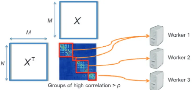
·jX·k < κ. These subsets A can then be safely as-signed to parallel worker machines (Fig. 3), and each machine will update the parameters j A sequentially (thus preventing depend-ency violations) [39].
Fig. 3. Illustration of ideal Lasso scheduling, in which parameter pairs (j, k) are grouped into subsets (red blocks) with low correlation between parameters in different subsets. Multiple subsets can be updated in parallel by multiple worker machines; this avoids violating dependency structures because workers update the parameters in each subset sequentially.
As for LDA, careful inspection reveals that the update equations ΔLDA for word token wij (Eq. (8)) may ① touch any element of column B·,wij, and ② touch any element of row δi,·. In order to prevent parallel worker machines from operating on the same columns/rows ofB and δ, we must partition the space of words {1,…, V} (correspond-ing to columns of B) into P subsets V1,…, VP, as well as partition the space of documents {1,…, N} (corresponding to rows of δ) into P subsetsD1,…, DP. We may now perform ideal data and model paral-lelization as follows: First, we assign document subset Dp to machine p out of P; then, each machine p will only Gibbs sample word tokens wij such that i Dp and wij Vp. Once all machines have finished, they rotate word subsets Vp among each other, so that machine p will now Gibbs sample wij such that i∈Dp and wij∈Vp+1 (or for ma-chine P, wij∈V1). This process continues until P rotations have com-pleted, at which point the iteration is complete (every word token has been sampled) [25]. Fig. 2 illustrates this process.
In practice, ideal schedules like the ones described above may not be practical to use. For example, in Lasso, computing XT·jX·k for all O(m2) pairs (j, k) is intractable for high-dimensional problems with large m (millions to billions). We will return to this issue shortly, when we introduce structure aware parallelization (SAP), a provably near-ideal scheduling strategy that can be computed quickly.
Compute prioritization in ML programs. Because ML programs
exhibit non-uniform parameter convergence, an ML scheduler has an opportunity to prioritize slower-to-converge parameters Aj, thus improving the progress per iteration of the ML algorithm (i.e., because it requires fewer iterations to converge). For example, in Lasso, it has been empirically observed that the sparsity-inducing l1 norm (Eq. (4)) causes most parameters Aj to ① become exactly zero after a few iterations, after which ② they are unlikely to become non-zero again. The remaining parameters, which are typically a small minority, take much longer to converge (e.g., 10 times more iterations) [39].
A general yet effective prioritization strategy is to select parame-ters Aj with probability proportional to their squared rate of change, (Aj(t– 1) –Aj(t– 2))2+ε, where ε is a small constant that ensures that stationary parameters still have a small chance to be selected. Depending on the ratio of fast- to slow-converging parameters, this prioritization strategy can result in an order-of-magnitude reduction in the number of iterations required to converge by Lasso regres-sion [39]. Similar strategies have been applied to PageRank, another iterative-convergent algorithm [53].
Balancing workloads in ML programs. When executing ML
programs over a distributed cluster, they may have to stop in order to exchange parameter updates, that is, synchronize—for example, at the end of Map or Reduce phases in Hadoop and Spark. In order to reduce the time spent waiting, it is desirable to load-balance the work on each machine, so that they proceed at close to the same rate. This is especially important for ML programs, which may ex-hibit skewed data distributions; for example, in LDA topic models, the word tokens wij are distributed in a power-law fashion, where a few words occur across many documents, while most other words appear rarely. A typical ML load-balancing strategy might apply the classic bin packing algorithm from computer science (where each worker machine is one of the “bins” to be packed), or any other strategy that works for operation-centric distributed systems such as Hadoop and Spark.
However, a second, less-appreciated challenge is that machine performance may fluctuate in real-world clusters, due to subtle reasons such as changing datacenter temperature, machine failures, background jobs, or other users. Thus, load-balancing strategies that are predetermined at the start of an iteration will often suf-fer from stragglers, machines that randomly become slower than the rest of the cluster, and which all other machines must wait for when performing parameter synchronization at the end of an
it-eration [37,40,60]. An elegant solution to this problem is to apply slow-worker agnosticism [38], in which the system takes direct advantage of the iterative-convergent nature of ML algorithms, and allows the faster workers to repeat their updates Δ while waiting for the stragglers to catch up. This not only solves the straggler problem, but can even correct for imperfectly-balanced workloads. We note that another solution to the straggler problem is to use bounded-asynchronous execution (as opposed to synchronous MapReduce-style execution), and we will discuss this solution in more detail in Section 3.2.
Structure aware parallelization. Scheduling, prioritization, and load balancing are complementary yet intertwined; the choice of parameters Aj to prioritize will influence which dependency checks the scheduler needs to perform, and in turn, the “independent subsets” produced by the scheduler can make the load-balancing problem more or less difficult. These three functionalities can be combined into a single programmable abstraction, to be implement-ed as part of a distributimplement-ed system for ML. We call this abstraction structure aware parallelization (SAP), in which ML programmers can specify how to ① prioritize parameters to speed up convergence; ② perform dependency checks on the prioritized parameters, and schedule them into independent subsets; and ③ load-balance the independent subsets across the worker machines. SAP exposes a simple, MapReduce-like programming interface, where ML pro-grammers implement three functions: ① “schedule(),” in which a small number of parameters are prioritized, and then exposed to dependency checks; ② “push(),” which performs ΔL in parallel on
worker machines; and ③ “pull(),” which performs F. Load balanc-ing is automatically handled by the SAP implementation, through a combination of classic bin packing and slow-worker agnosticism.
Importantly, the SAP schedule() does not naively perform O(m2) dependency checks; instead, a few parameters A are first selected via prioritization (where A<<m). The dependency checks are then performed on A, and the resulting independent subsets are updated via push() and pull(). Thus, SAP only updates a few parameters Aj per iteration of schedule(), push(), and pull(), rather than the full model A. This strategy is provably near-ideal for a broad class of model par-allel ML programs:
Theorem 1 (adapted from Ref. [35]):SAP is close to ideal exe-cution.Consider objective functions of the formL = f(A) + r(A), where r(A) = jr(Aj)is separable,A Rd, and f has β-Lipschitz continuous gradient in the following sense:
(
)
( )
( )
T T T
2 f A z+ ≤f A + ∇z f A +βA X Xz
(13)
Let X = [x1,…,xd] be the data samples re-represented as d feature
vec-tors. W.l.o.g., we assume that each feature vector xi is normalized, that is, xi 2=1, i = 1,…, d. Therefore, x xiT j ≤1for all i and j.
Suppose we want to minimizeLvia model parallel coordinate de-scent. LetSideal() be an oracle (i.e., ideal) schedule that always proposes P random features with zero correlation. Let A ideal( )t be its parameter trajectory, and let A SAP( )t be the parameter trajectory of SAP scheduling. Then, ( ) ( )
(
)
2 T ideal SAP 2 2 ˆ 1 t t dPm L C t P − ≤ A A + X X (14)for constants C, m, L,andPˆ.
This theorem says that the difference between the SSAP() parame-ter estimate ASAP and the ideal oracle estimate Aideal rapidly vanishes, at a fast 1/(t+ 1)2 = O(t–2) rate. In other words, one cannot do much better than SSAP() scheduling—it is near-optimal.
SAP’s slow-worker agnostic load balancing also comes with a theoretical performance guarantee—it not only preserves correct ML convergence, but also improves convergence per iteration over naive scheduling:
agnosti-cism improves convergence progress per iteration.Let the current variance (intuitively, the uncertainty) in the model beVar (A), and let np > 0be the number of updates performed by worker p (including additional updates due to slow-worker agnosticism). After np updates,
Var (A)is reduced to
( )
( )
( )
(
)
(
)
2 1 2 3Var Var Var CoVar ,
cubic p n t p t p t p c n c n c n O η η η + = − − ∇ + + A A A A L (15)
where, ηt > 0is a step-size parameter that approaches zero as t→∞; c1, c2, c3> 0 are problem-specific constants; Lis the stochastic gradient of the ML objective functionL;CoVar(a, b)is the covariance between a and b, and O(cubic)represents third-order and higher terms that shrink rapidly toward zero.
A low variance Var (A) indicates that the ML program is close to convergence (because the parameters A have stopped changing quickly). The above theorem shows that additional updates np do indeed lower the variance—therefore, the convergence of the ML program is accelerated. To see why this is the case, we note that the second and third terms are always negative; furthermore, they are O(ηt), so they dominate the fourth positive term (which is O(ηt2) and therefore shrinks toward zero faster) as well as the fifth positive term (which is third-order and shrinks even faster than the fourth term).
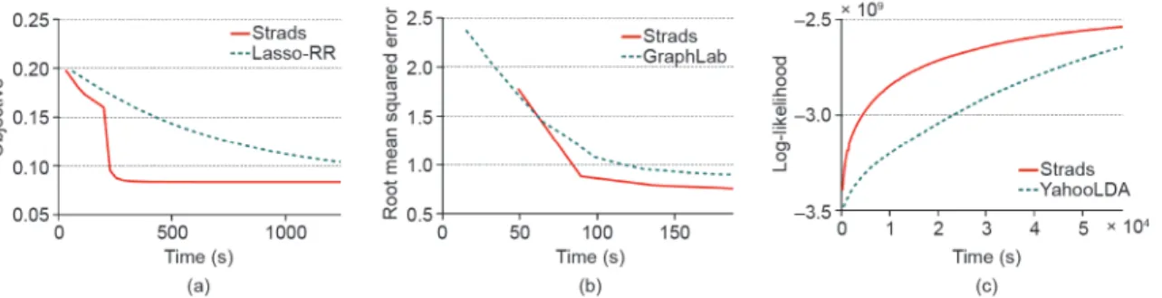
Empirically, SAP systems achieve order-of-magnitude speedups over non-scheduled and non-balanced distributed ML systems. One example is the Strads system [39], which implements SAP schedules for several algorithms, such as Lasso regression, matrix factorization, and LDA topic modeling, and achieves superior convergence times compared to other systems (Fig. 4).
3.2. How to bridge computation and communication: Bridging models and bounded asynchrony
Many parallel programs require worker machines to exchange program states between each other—for example, MapReduce sys-tems such as Hadoop take the key-value pairs (a, b) created by all Map workers, and transmit all pairs with key a to the same Reduce worker. For operation-centric programs, this step must be exe-cuted perfectly without error; recall the MapReduce sort example (Section 2), where sending keys to two different Reducers results in a sorting error. This notion of operational correctness in parallel programming is underpinned by the BSP model [61,62], a bridg-ing model that provides an abstract view of how parallel program computations are interleaved with inter-worker communication. Programs that follow the BSP bridging model alternate between a computation phase and a communication phase or synchronization barrier (Fig. 5), and the effects of each computation phase are not visible to worker machines until the next synchronization barrier
has completed.
Because BSP creates a clean separation between computation and communication phases, many parallel ML programs running under BSP can be shown to be serializable—that is to say, they are equiva-lent to a sequential ML program. Serializable BSP ML programs enjoy all the correctness guarantees of their sequential counterparts, and these strong guarantees have made BSP a popular bridging model for both operation-centric programs and ML programs [32,34,63]. One disadvantage of BSP is that workers must wait for each other to reach the next synchronization barrier, meaning that load bal-ancing is critical for efficient BSP execution. Yet, even well-balanced workloads can fall prey to stragglers, machines that become ran-domly and unpredictably slower than the rest of the cluster [60], due to real-world conditions such as temperature fluctuations in the datacenter, network congestion, and other users’ programs or background tasks. When this happens, the program’s efficiency drops to match that of the slowest machine (Fig. 5)—and in a cluster with thousands of machines, there may even be multiple stragglers. A second disadvantage is that communication between workers is not instantaneous, so the synchronization barrier itself can take a non-trivial amount of time. For example, in LDA topic modeling running on 32 machines under BSP, the synchronization barriers can be up to six times longer than the iterations [37]. Due to these two disadvantages, BSP ML programs may suffer from low iteration throughput, that is, P machines do not produce a P-fold increase in throughput.
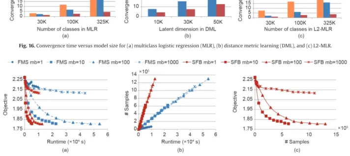
As an alternative to running ML programs on BSP, asynchronous parallel execution (Fig. 6) has been explored [28,33,52], in which worker machines never wait for each other, and always commu-nicate model information throughout the course of each iteration. Asynchronous execution usually obtains a near-ideal P-fold increase in iteration throughput, but unlike BSP (which ensures serializability and hence ML program correctness), it often suffers from decreased Fig. 4. Objective function L progress versus time plots for three ML programs—(a) Lasso regression (100M features, 9 machines), (b) matrix factorization (MF) (80 ranks, 9 ma-chines), (c) latent Dirichlet allocation (LDA) topic modeling (2.5M vocab, 5K topics, 32 machines)—executed under Strads, a system that realizes the structure aware paralleli-zation (SAP) abstraction. By using SAP to improve progress per iteration of ML algorithms, Strads achieves faster time to convergence (steeper curves) than other general- and special-purpose implementations—Lasso-RR (a.k.a., Shotgun algorithm), GraphLab, and YahooLDA. Adapted from Ref. [39].
Fig. 5. Bulk synchronous parallel (BSP) bridging model. For ML programs, the worker machines wait at the end of every iteration for each other, and then ex-change information about parameters Aj during the synchronization barrier.
convergence progress per iteration. The reason is that asynchronous communication causes model information to become delayed or stale (because machines do not wait for each other), and this in turn causes errors in the computation of Δ and F. The magnitude of these errors grows with the delays, and if the delays are not carefully bounded, the result is extremely slow or even incorrect convergence
[37,40]. In a sense, there is “no free lunch”—model information must
be communicated in a timely fashion between workers.
BSP and asynchronous execution face different challenges in achieving ideal P-fold ML program speedups—empirically, BSP ML programs have difficulty reaching the ideal P-fold increase in iter-ation throughput [37], while asynchronous ML programs have dif-ficulty maintaining the ideal progress per iteration observed in se-quential ML programs [25,37,40,]. A promising solution is bounded- asynchronous execution, in which asychronous execution is permit-ted up to a limit. To explore this idea further, we present a bridging model called stale synchronous parallel (SSP) [37,64], which gener-alizes and improves upon BSP.
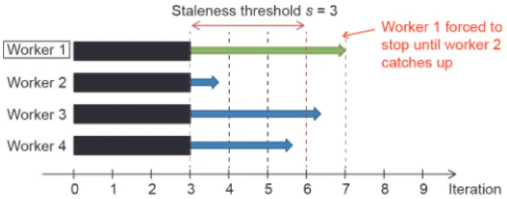
Stale synchronous parallel. Stale synchronous parallel (SSP) is a bounded-asynchronous bridging model, which enjoys a similar pro-gramming interface to the popular BSP bridging model. An intuitive, high-level explanation goes as follows: We have P parallel workers or machines that perform ML computations Δ and F in an iterative fashion. At the end of each iteration t, SSP workers signal that they have completed their iterations. At this point, if the workers were instead running under BSP, a synchronization barrier would be enacted for inter-machine communication. However, SSP does not enact a synchronization barrier. Instead, workers may be stopped or allowed to proceed as SSP sees fit; more specifically, SSP will stop a worker if it is more than s iterations ahead of any other worker, where s is called the staleness threshold (Fig. 7).
More formally, under SSP, every worker machine keeps an iteration counter t, and a local view of the model parameters A.