Self-organizing networks

(1)

B.Eng. Thesis Bachelor of Engineering

Self-Organizing Networks

Energy Saving

Maria Gonzalez Calabuig

s175943

(2)

Author

Maria Gonzalez Calabuig

Supervisors

Henrik Lehrmann Christiansen Matteo Artuso

Ramon Ferrús Ferré

Project Details

Start date: January 29th 2018 End date: June 22nd 2018 Defense date: July 2nd 2018 Credits: 20 ECTS points

DTU Fotonik

Department of Photonics Engineering Technical University of Denmark

Ørsteds Plads Building 343

2800 Kongens Lyngby, Denmark Phone +45 4525 6352

(3)

Abstract

Due to the growth of mobile traffic data, networks are becoming more complex sys-tems. In order to provide service for all the users and maintain a good quality of service, new infrastructure is deployed and more complex protocols are developed. In this situation, operators face a rise in operational and capital expenditures.

Self-Organizing Networks appear as a solution to reduce these expenditures as well as to improve the utilization of the resources. These type of networks provide certain level of autonomy to the network, minimizing the human intervention in dif-ferent functions and providing autonomous and adaptive solutions.

The concept and its characteristics is presented in this thesis, focusing in a partic-ular use case: Energy Saving.

The thesis narrows down from the general concept of Self-Organizing Networks to the concrete use case of Energy Saving. The document provides an overview of Self-Organizing Networks followed by the study of the Self-Optimization category and ending with an extensive discussion of the Energy Saving use case.

Furthermore, the simulation and results of an algorithm implementing an Energy Saving solution are presented, with an evaluation of its performance in order to deter-mine if it obtains energy efficiency. Without degrading the network performance, a reduction up to 45% of consumed power can be obtained with the proposed algorithm.

(4)

Preface

This thesis was prepared at the Fotonik department at the Technical University of Denmark in fulfillment of the requirements for acquiring a Bachelor’s degree in Telecommunications Technologies and Services Engineering.

Kongens Lyngby, June 22, 2018

(5)

Acknowledgements

I would like to offer my special thanks to my co-supervisors, Dr. Henrik Lehrmann Christiansen, Dr. Matteo Artuso and Dr. Ramon Ferrús Ferré for all the given advises. Their willingness to give their time, disposition to help and answer my ques-tions is very much appreciated.

I wish to thank the Polytechnic University of Catalonia and the Technical Univer-sity of Denmark for offering me this opportunity and making it a reality.

Finally, I would also like to thank my family, friends from home and all the new friends made during these few months for all the trust deposited on me.

(6)

Acronyms

3GPP 3rd Generation Partnership Project ACK Acknowledgment

ANR Automatic Neighbour Relationship BBU Baseband Unit

CAPEX Capital Expenditures

CCO Coverage and Capacity Optimization CIO Cell Individual Offset

CQI Channel Quality Indicator DL Downlink

DMR Detection Miss Ratio eNB Evolved Node B

ECGI E-UTRAN Cell Global Identifier ES Energy Saving

ESM Energy Saving Management

E-UTRAN Evolved Universal Terrestrial Radio Access Network FDD Frequency Division Duplexing

GHG Global Green-House Gas

HARQ Hybrid Automatic Repeat Request HO Handover

IC Interference Control

ICT Information and Communication Technology ITU International Telecommunication Union LOS Line of Sight

LTE Long Term Evolution MLB Mobility Load Balance

MRO Mobility Robustness Optimization NACK Non-Acknowledgment

NCBRA Non-Contention based Random Access NE Network Element

NLOS Non-Line of Sight

NRT Neighbour Relation Table OPEX Operating Expenditures O&M Operation And Maintenance PCI Physical Cell Identity

PUSCH Physical Uplink Shared Channel QoS Quality of Service

(9)

Acronyms vii

RACH Random Access Channel RAT Radio Access Technologies RF Radio Frequency

RNC Radio Network Controller SNR Signal to Noise Ratio SON Self-Organizing Networks TCI Target Cell Identifier TTT Time-to-Trigger UE User Equipment UL Uplink

(10)

List of Figures

1.1 Mobile Data Traffic by 2021 by Cisco (47% CAGR) [1] . . . 1

1.2 Mobile Devices by 2021 by Cisco (20% CAGR) [1] . . . 1

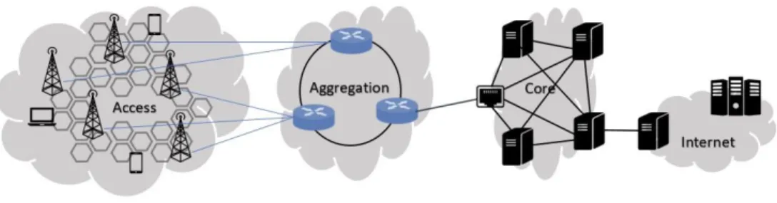
2.1 Network architecture . . . 3

2.2 Simplified diagram of the interaction of the SON’s categories adapted from [5] [6] . . . 4

2.3 Time scale classification adapted from [4] . . . 6

2.4 SON architectures adapted from [10] . . . 7

2.5 ANR functions scheme adapted from [12] . . . 8

3.1 Random Access procedures . . . 11

3.2 Downlink inter-cell interference . . . 15

3.3 Uplink inter-cell interference . . . 16

3.4 Use Cases’ intersections . . . 17

4.1 Mobile operator’s energy consumption adapted from [38] . . . 22

4.2 BS Components power consumption adapted from [38] . . . 22

4.3 Energy Saving Management states . . . 26

5.1 Example of a simulation layout with 5 base stations and 3 users . . . 32

5.2 Example of the dependence between the state variation and utilization thresholds in a time scale . . . 35

5.3 Energy Saving states . . . 36

5.4 Consumption of the Macro base station with loThr=20 . . . 38

5.5 Consumption of the Micro base stations withloThr=20 . . . 39

5.8 Number of HARQ retransmissions per base station using different thresholds 41 5.9 Total number of HARQ retransmissions in the network . . . 42

(11)

List of Tables

3.1 Parameters optimized by each use case . . . 17

3.2 Optimization effect . . . 19

5.1 Fixed Simulations parameters of the base stations . . . 37

5.2 Fixed Simulations parameters of a User . . . 37

(12)

1

Introduction

1.1 Problem Statement

During the past years, mobile data traffic has grown exceeding all expectations. By 2021, there will be 11,6 billion mobile-connected devices and the mobile data traffic will have increased a 47% since 2016 [1]. On figure Figure 1.1 and Figure 1.2, it can be seen the mobile data traffic growth estimated by Cisco as well as the number of the increase in number of devices.

Figure 1.1: Mobile Data Traffic by 2021 by Cisco (47% CAGR) [1].

Figure 1.2: Mobile Devices by 2021 by Cisco (20% CAGR) [1].

Operators have to keep up with the demand, providing coverage for all new de-vices and improving the service provided to the user. For this purpose, networks are becoming more complex systems as new infrastructure is deployed and more complex protocols are being developed.

In this situation, Self-Organizing Networks appear as a potential solution to re-duce the operative and capital expenditures. A Self-Organizing Network provides a level of autonomy to the network allowing a set of functions to perform with minimum human intervention and adapt to the changes of the network.

Apart from the cost that supposes the deployment of new infrastructures and exe-cution of new protocols, a major concern for society appears linked to these significant

(13)

1.2 Project Scope 2

changes: the environmental impact.

The network infrastructure has great impact on the environment. Society de-mands to take action on two main factors: the hardware elements and the energy consumption. The elements have to be obtained in a sustainable way, either by recy-cling other disposed artifacts or with conflict-free and non harmful materials. At the end of their life cycle, their recycling or deposition as to be easy and feasible. On the other hand, energy consumption should be minimized as much as possible [2].

The objective of the Energy Saving use case, fitting in the Self-Optimizing category of Self-Organizing Networks, takes action on the second factor mentioned above.

1.2 Project Scope

The objective of this project is to provide a theoretical background about the concept of Self-Organizing Networks, more precisely, on the Energy Saving use case. For this reason, the main topic, Self-Organizing Networks, is broken down and sequentially explained until the Energy Saving use case is reached.

A small section of the thesis provides the results of an Energy Saving algorithm, completing the whole picture for this use case. Due to time and resource limitations, the experiment only presents the simulation of one scenario.

1.3 Thesis outline

The report is organized in six chapters.

Chapter 2 introduces the concept of Self-Organizing Networks along with its tax-onomies and standards.

Chapter 3 focuses on the use cases of the Self-Optimization category. A brief explanation and related works of each use case are presented.

In Chapter 4, the characteristics of the Energy Saving use case are exposed. Ex-amples of research works are summarized at the end of the chapter.

Chapter 5 evaluates and analyses an Energy Saving algorithm in means of energy efficiency.

(14)

2

Self-Organizing Networks

The acronym SON stands for Self-Organizing Networks. A Self-Organizing Network is an automated adaptative network, capable of performing a set of functions with the minimum human intervention.

This chapter is an introduction to the SON concept. Firstly, what motivated the appearance of this concept is exposed. Afterwards, the use cases and taxonomies are explained. The last section focuses on the standardized features.

2.1 Motivation

Providing service to a user is a complex procedure with a lot of parties included. There are multiples parameters to take into account as well as a great number of protocols and technologies operating at the same time.

Figure 2.1: Network architecture.

The more the network expands, the more complex the system is [3]. A complex system requires more supervision so operating expenses (OPEX) increase. At the same time, human supervision is tied to human errors which degrade the service pro-vided to the users. Finally, as there are multiple protocols and functions, conflicts may arise, damaging the network performance. The Self-Organizing Network concept appears as a solution to these issues [4].

(15)

2.2 SON Taxonomy: Use Cases 4

A self-organizing network provides a certain level of autonomy to the network. The benefits are many; improving the usage of the network’s resources can be di-rectly translated in a decrement of OPEX and, also, as explained in [2], “Practical experience shows that the application of 3G SON technologies in current UMTS infrastructure can yield a capacity gain of 50% without carrying out any CAPEX expansion.”.

With the improvement of the network’s features and the saving in capital, SON becomes a potential solution to the different problems mentioned above.

2.2

SON Taxonomy: Use Cases

SON applications, commonly known as SON Use Cases, are classified in different categories. Although there is no official classification, the one that will be followed through this document, groups the use cases in three categories: Self-Configuration, Self-Optimization and Self-Healing. The interaction of the categories between each other has been pictured on Figure 2.2:

Figure 2.2: Simplified diagram of the interaction of the SON’s categories adapted from [5] [6].

2.2.1 Self-Configuration

The Self-Configuration of a network includes the functions needed for the prepara-tion of the deployment of the different nodes that conform it. This category is also in

(16)

2.2 SON Taxonomy: Use Cases 5

charge of the set-up of the network; that includes preparation, installation, authenti-cation and verifiauthenti-cation of the nodes.

In this category, the use cases are [7] [8]:

− Intelligently selecting site locations, detect degradation during operation and provide a solution.

− Automatic generation of default parameters for NE insertion,provides a default set of radio network related parameters to a newly installed NE.

− Network authentication, establishment of mutual authentication between the eNB and the network.

− Hardware/capacity extension,allows the continuity of service when a eNB is having new hardware installed.

− Automated Configuration of Physical Cell Identity,automated selection of the Physical Cell Identity when a eNB is newly deployed. The selection has to avoid any collision with the neighbouring cells when selecting the identifier.

− Automatic Neighbour Relation Function,builds the Neighbour Relations Table containing all the neighbour eNBs.

2.2.2

Self-Optimization

The Self-Optimization category has the purpose of tuning the network setting once the network is in the operating state. This category covers a wide number of Use Cases. Some examples are the optimization of the neighbour list, interference con-trol, optimization of handover parameters, load balance, optimization of QoS-related parameters, energy saving, etc.

This category will be further discussed in chapter 3.

2.2.3

Self-Healing

Self-Healing oversees preventing or repairing any arising problem. It is centred on the maintenance performance done by an operator. Its Use Cases cover:

− Hardware extension/replacement,providing service and granting its qual-ity while the hardware is replaced.

− Software upgrade,installation of new software updates.

− Network monitoring,which consists of performing measurements and analy-sis to the network in order to recognize insufficiencies or needed improvements.

(17)

2.3 Alternative Taxonomies 6

2.3

Alternative Taxonomies

The use cases classification presented above is a phase based classification. The use cases are classified depending on which phase they work on. The three phases, Self-Configuration, Self-Optimization and Self-Healing, correspond to the three phases of the life of a base station: deployment, optimization and maintenance. But this is not the only existing classification [4].

Another possible way of classifying use cases is the time scale. The use case’s algorithms operate on different time scales depending on the part of the network where it is executed. On Figure 2.3 the different time scales are represented:

Figure 2.3: Time scale classification adapted from [4].

It is also possible to classify them depending on the objective of the self-organizing algorithms. This approach’s problem is that the same algorithm may be used to or-ganize multiple use cases.

Finally, some authors have classified the use cases according to the conflicts [9]. Firstly, this classification identifies the potential conflicts between Self-Organizing functions. Later, the conflicts get categorized. The principal issue of this method is the repetition of use cases. A use case can cause different types of conflicts.

(18)

2.4 3GPP Standardized Features 7

2.4

3GPP Standardized Features

The 3GPP (3rd Generation Partnership Project) is a union of telecommunications standard development organizations which provide reports with Requirements and Specifications that define technologies. The project has worked with the SON, stan-dardizing its features in terms of architecture, actor roles along with other require-ments.

2.4.1 Architecture

Depending on where the SON function take place, the architecture type can be clas-sified in three groups [7]:

Figure 2.4: SON architectures adapted from [10].

− Centralized, the SON functions are located in the O&M system, in the core network. In this category, the algorithms can be executed at the Network Management level or at the Element Management level.

− Distributed (De-centralized), when the SON functions are performed by the eNodeB, a distributed architecture is being used.

− Hybrid, this type of architecture combines a set of SON functions, placed on different levels on the O&M hierarchy.

2.4.2

Framework

There are some SON functionalities already standardized. The Automatic Neighbour Relationship and the Plug-and-Play are an example. These use cases are used by the research community has a framework when implementing other SON functionalities.

(19)

2.4 3GPP Standardized Features 8

2.4.2.1 Automatic Neighbour Relationship

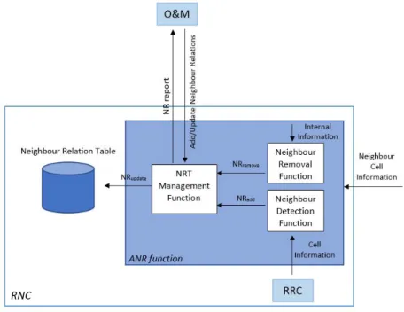
The Automatic Neighbour Relationship (ANR) configures the neighbour list of an eNB newly deployed and updates it while the base station is operative. This use case fits in two categories: Self-Configuration and Self-Optimization. When the eNB is deployed, the ANR mission is to minimize the required work for its configuration while, when already operative, the ANR mission is to optimize the configuration [11]. Figure 2.5 shows the different parts and the interaction between each part:

Figure 2.5: ANR functions scheme adapted from [12].

The ANR is divided in three functions: Neighbour Removal, Neighbour Detection and NRT Management. ANR follows a distributed architecture, all functions take place in the RNC, node which connects with the core network.

The neighbour removal and detection are responsible of deciding if it is needed to add or remove an entry on the Neighbour Relation Table (NRT). Each entry of the NRT is a neighbour base station which is identified by a unique Target Cell Identifier (TCI). The TCI includes the PCI and the E-UTRAN Cell Global Identifier (ECGI) [2].

The NRT Management is the function which will update the NRT after a decision is made. This last function is also coordinated by the O&M, situated in the core network, which can also decide if the NRT has to be updated.

(20)

2.5 Summary 9

2.4.2.2 Plug-and-Play

The Plug-and-Play use case reduces the effort of deploying a base station, the only manual required acction is the physical installation of the sites. Only the deployment is required while all other functions are executed automatically. The eNB configures the Physical Cell Identity, transmission frequency and power, S1 and X2 interfaces, IP address and connection to IP backhaul [11] [13]. The Plug-and-Play covers different use cases of the Self-Configuration category.

2.5

Summary

The concept of SON appears motivated by the reduction of OPEX and CAPEX. As traffic grows, more complex networks are needed. The complexity of these systems may exceed human capacity of controlling and exploiting all the resources of the net-work. A self-organizing network reduces OPEX, as some functions are automatized and may only require minimum human intervention, and, also, reduces CAPEX, as a better usage of the resources can be done and, therefore, the service may improve without the need of deploying more infrastructures.

organizing networks are divided in three categories: Configuration, Self-Optimization and Self-Healing. Each one of these categories cover different use cases.

Even though the previous taxonomy is the most common, there exist other classi-fications. The use cases can be classified by time scale, objective or conflicts.

The 3GPP project standardized the SON architecture in three variants, depending on where the SON algorithms take place. It can be a centralized, distributed or hybrid architecture. Also, the same project has already proposed solutions for some use cases such as Automatic Neighbour Relationship or Plug-and-Play.

(21)

3

Self-Optimization Use Cases

As explained on the previous section, the Self-Optimization category covers the tuning of the network once it is in the operating mode. This chapter will take a deeper look at the Use Cases of most interest to the research community on this category [14]:

− RACH Optimization

− Mobility Robustness Optimization − Mobility Load Balancing

− Coverage and Capacity Optimisation − Interference Control

− Energy Saving

After explaining each use case and providing some examples of research works, a discussion will take place. The analysis of each optimization along with the com-patibility between use cases will be dicussed to provide a general over view of the Self-Optimization category.

3.1 RACH Optimization

An UE trying to access the network for the first time has to perform a Random Access Procedure. The information exchange for this procedure is done through the Random Access Channel (RACH), which is shared with other UEs.

An UE will perform a Random Access on four situations: 1) initial access when in Idle mode, 2) handover to a different cell, 3) re-establishment of the radio link after radio link failure and 4) uplink or downlink data transmission when the UE has no synchronization on the uplink [15].

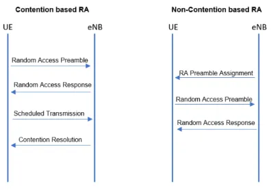
Two scenarios can take place when the UE is requesting the access. On the first one, there could be another UE requesting access at the same time and, therefore, a collision. This scenario is called Contention based Random Access procedure. On the second scenario, the network can notify a preamble sequence to the UE, to prevent any collision with others UEs. In this case, a Non-Contention or Contention free based Random Access procedure would be used.

(22)

3.1 RACH Optimization 11

Figure 3.1: Random Access procedures.

A preamble sequence is a specific pattern which differentiates UEs. As specified in [15], the total number of RACH preambles available in LTE is 64.

In a network, optimal RACH performance is essential in order to obtain higher coverage and lower delays. The number of resources allocated to random access has a direct impact on the delays. Allocating a larger number of resources involves lower collision probability. This translates on lower delays but at the same time, the UL capacity is also lowered. The Random Access performance can be expressed on terms of Access Probability and Access Delay Probability.

In the existent literature, different approaches have been taken to improve the access probability and the access delay probability. Most of the research on this field is based on the evaluation of a parameter of the Random Access procedure and a proposal of an algorithm focused on that unique parameter. The RACH parameters that can be optimized are resource unit allocation, preamble split, back off parameter value and transmission control parameters [5]. These parameters can be different on each cell and time variant. Some of the approaches can be seen on [16, 17, 18, 15].

In [16], through simulations, the benefits of optimization and self-tuning of RACH parameters is proved. The dependence between RACH parameters and the Detection Miss Ratio and Contention Ratio is evaluated. These parameters are the PUSCH Load, the RACH Load, the power ramping step and the interference on PUSH gen-erated by the preamble transmissions. Finally, a Self-tuning algorithm for energy saving is proposed. By automatically adjusting the desired received power, the DMR can be controlled to meet a given performance. This algorithm gives room to im-provement by adjusting the other evaluated parameters.

(23)

3.2 Mobility Robustness Optimization 12

On the other hand, on [17] the study is focused on the uplink resource allocation depending on the traffic changes. The proposed algorithm tries to improve the uplink capacity to ensure a success rate at the random access first attempt. That implies reducing the handover and call setup delays.

Following that, on [18] the resource allocation optimization is approached by the configuration of RACH subframes given the arrival rate. If two users transmit the same preamble on the same RACH subframe, there will be a collision. Both users will have to retransmit the random access preambles. By adjusting the number of subframes allocated on the RACH, the collision probability is lowered and, therefore, the access delay.

Finally, the authors on [15] focus on preamble split. Three algorithms are pro-posed to improve the Random Access success rate. On the first algorithm, the avail-able preambles are split based on the ratio of Non-Contention based Random Access to the total random accesses (NCBRA ratio). The second algorithm proposes an improvement by considering the access failure rate. The last algorithm also provides an improvement by considering the random access arrival rate.

3.2 Mobility Robustness Optimization

While a mobile device is connected to the network, it measures the signal strength of neighbouring cells. Based on the device’s reports, the eNodeB can take the decision of performing a handover, which consists of handing over the connection to a neigh-bour cell with a better signal. The handover procedure prevents the connection from dropping and improves the data throughput.

The Mobility Robustness Optimization use case focuses on improving the handover process. The problems in which MRO focuses are the following ones [5]:

− Connection failure due to intra-LTE or inter-RAT mobility:

The connection failure can be due a too early HO, due to a too late HO or due to a HO to a wrong cell.

− Unnecessary HO to another RAT (too early IRAT HO with no radio

link failure):

It can happen that the UE is handed over from E-UTRAN to another RAT (eg. UTRAN or GERAN) even though the coverage was sufficient for the service. Therefore, the handover may be considered unnecessary.

− Inter-RAT ping-pong:

An UE can perform a handover from a cell in a source RAT to another cell with a different RAT, then, after a limited amount of time, the UE is handed back to the source cell again. This event may happen more than one time.

(24)

3.3 Mobility Load Balancing 13

The parameters that can be optimized by the MRO functionality are the time to trigger, hysteresis, cell individual offset, frequency-specific offset and cell reselection parameters [14]. These parameters are used for tuning the triggering of the measure-ment report events [19]:

A1: Serving becomes better than the threshold. A2: Serving becomes worse than threshold. A3: Neighbour becomes offset better than serving. A4: Neighbour becomes better than threshold.

A5: Serving becomes worse than threshold1 and neighbour becomes better than threshold2.

B1: Inter RAT neighbour becomes better than threshold.

B2: Serving becomes worse than threshold1 and inter RAT neighbour becomes better than threshold2.

In the literature, most of the research is centred on the improvement of the con-netion to avoid failure. The approach taken in [20] provides a solution by adaptatively modifying the hysteresis parameters depending on the user speed. Most recent works, such as [21], focus on adapting the time-to-trigger, cell individual off-sets and A3 parameters according to the dominant handover failure (too late, too early or wrong cell handover).

On the other hand, [22] approaches the problems of inter-RAT handovers. These problems are ping-pong effect and connexion failure. The parameters that are modi-fied in this case are the event thresholds, time-to-trigger and filter coefficients. Their conclusion is that the MRO has to work locally on each cell, as the mobility condi-tions differ. Inter-RAT handovers are more sensitive to changes on the B2 threshold 1 than on the TTT.

3.3 Mobility Load Balancing

The number of users on a cell and the data usage of each of them can be modelled as random variables that differ depending on the date or time. This leads to unequal load scenarios for neighbouring cells. It may happen that, at a given time, a cell is overloaded, while its neighbour cell is underloaded. The quality of the service on the overloaded cell may not meet the QoS requirements while, on the underload cell, the resources are not being fully used.

(25)

3.4 Coverage and Capacity Optimization 14

The Mobility Load Balancing feature is in charge of detecting the load imbalance and reassigning the users on all the available cells within a zone. This way, an efficient usage of the radio resources of the network is performed while granting the quality of service of the users. The Load balancing can be performed in two scenarios [14]:

− Intra-LTE Load Balancing.

− Inter-RAT Load Balancing.

In both scenarios, the eNodeBs need to have information about the load of the neighbour cells to take the appropriate action for the loading balance. On the Intra-LTE scenario, the eNodeBs exchange load information through the X2 interface while on the Inter-RAT scenario, the information exchange is done through the S1 inter-face. These reports are also essential to avoid unnecessary handovers and inter-RAT ping-pong handovers.

This use case is strongly tied to Mobility Robustness Optimization. As said be-fore, this use case focuses on reallocating the load of a zone and, to do so, it is needed to tune handover parameters. This way, users on overloaded cells can be forced into underloaded neighbouring cells and, thus, re-distribute the load. Some researches that approach this issue are [23, 24, 25].

In [23] they refer to their algorithm asNeighbourhood mobility load balance. This algorithm tries to find the Cell Individual Offset (CIO) that maximises the offload of the overloaded cell. The research’s conclusion is that, by using their algorithm, considerable gain on the QoS of the users is achieved at the expense of reducing the spectral efficiency. In [24], the proposed algorithm (Zone-based mobility load balanc-ing) tries to distribute uniformly the excess of traffic on all the neighbour cells of the overloaded cell, in comparation to the conventional MLB, which focuses on transfer-ring the traffic only to one of the neighboutransfer-ring cells.

Finally, in [25], the research is focused on the A3 handover event. The proposed al-gorithm (Inter-frequency load balancing) tunes the handover thresholds and frequency-specific offsets in order to trigger the handover from an overloaded cell to an under-loaded cell.

3.4 Coverage and Capacity Optimization

The Coverage and Capacity Optimization use case focuses on providing the optimal coverage and capacity while the network is operative. Coverage and Capacity prob-lems may arise due to five causes [26]:

− Coverage hole:

Area where the UE cannot access the network due to the low pilot signal strength. It may be caused by physical obstacles or inadequate RF planning.

(26)

3.5 Interference Control 15

− Weak coverage:

Pilot signal strength or SNR below the level to maintain a planned performance requirement.

− Pilot pollution:

High interference and energy consumption with a low cell performance due to overlapping cells.

− Overshoot coverage:

Due to reflections on buildings or lakes, the coverage of a cell may reach far beyond what was planned causing high interference and call drops.

− DL and UL channel coverage mismatch:

DL channel coverage larger than the UL channel coverage.

The parameters that can be tuned to obtain the optimal coverage and capacity are the downlink transmit power, antenna tilt and antenna azimuth.

Most of the existing works approach the issue by adjusting the antenna’s tilt [27, 28, 10, 29]. In [30], the authors affirm that “Adjusting the antenna tilt is one of the most powerful techniques to solve coverage and capacity problems in cellular networks”.

3.5 Interference Control

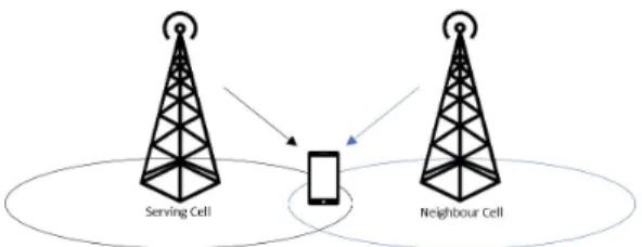
The Interference Control use case focuses on reducing the impact of the transmission on neighbour cells. In LTE, all cells reuse the same carrier frequencies [31]. While an UE is near the station of the serving cell, the received power of this cell will be higher than the received power of the neighbour cells using the same carrier frequency. Problems arise when the UE is on the edge of two or more coverage areas. The received power from neighbour cells will be higher and the interference it causes will be considerable. This would be called Downlink inter-cell interference.

Figure 3.2: Downlink inter-cell interference.

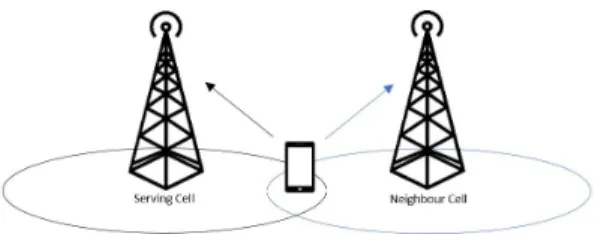
At the same time, the UE can cause interference to the neighbour cell, as it also sends information to all the other cells apart from the serving one. In this case, the

(27)

3.6 Energy Saving 16

UE would be causing Uplink inter-cell interference. On the cell edge, the interference is higher.

Figure 3.3: Uplink inter-cell interference.

The Interference Control has to take into account both scenarios and reduce the interference to increase the capacity and quality of service of the users.

The studies that confront this use case mainly focus on Optimization of Spectrum Allocation or Optimization of Power Settings. In [32], after summarizing the related works, their proposed algorithm regulates the transmitted power according to the channel quality indicator (CQI) received from the user. The CQI is computed based on the SINR from the received interference.

On the other hand, in [33], they present a solution with an optimization module that improves sectorization, antenna angle selection and spectrum allocation. After that, a second module, called power allocation module, finds the best relation between capacity and interference.

3.6 Energy Saving

The main objective of the Energy Saving is the reduction of the energy consumption. This can be obtained by matching the offered capacity with the needed traffic demand at any given time while the network is operative [14].

The Support to the Energy Saving use case, on the 3GPP, specification [5] defines a switching-off solution based on cell load information. To effectuate the switch-off, the eNB has to have a general oversight of the situation of all neighbouring cells.

(28)

3.7 Use Cases Compatibility 17

3.7

Use Cases Compatibility

After a summarized explanation of the major use cases of the Self-Optimization cat-egory, it has been seen that some of them modify the same type of parameters (e.g. Handover parameters). This may lead to the question whether the different use cases are compatible with each other.

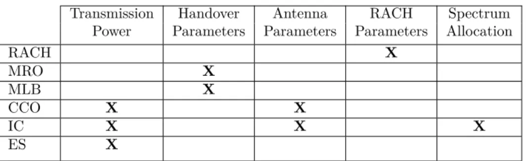
The following table has been extracted from the previous sections. In it, it can be seen which parameters are optimized by each use case.

Table 3.1: Parameters optimized by each use case.

Transmission Handover Antenna RACH Spectrum Power Parameters Parameters Parameters Allocation

RACH X MRO X MLB X CCO X X IC X X X ES X

From the table, the intersections can be depicted, as it can be seen in Figure 3.4 Notice that the information of the table can vary, as new approaches for the use case can be taken.

Figure 3.4: Use Cases’ intersections.

Three groups are obtained. The use cases that do not share parameters are com-patible with each other but the ones that share parameters have to be carefully im-plemented. One clear example is the intersection between MRO and MLB. Both use cases modify handover parameters. If they modify the same parameter on opposite directions a conflict will arise, ping-pong effect with both functions will appear and an inefficient use of the functions will be done, degrading the service. The same

(29)

hap-3.7 Use Cases Compatibility 18

pens with IC, Energy Saving and Coverage and Capacity optimization. The three use cases work on the adaptation of the transmitted power. If a use case tries to increase the power to increase the coverage area, the IC may try to decrease it to minimize the interference or the Energy Saving may try to reduce the energy consumption by doing the same. At the same time, with this last example, the Energy Saving and IC could be compatible as both achieve their objective by reducing the transmitted power.

That is why knowing which parameters they have in common is not enough, a deeper analysis has to be done. Figure 3.4 could be interpreted in different way, as the effect of each modification on the other use cases has to be taken into account.

The use cases improve some features at the expense of lowering some other ones. As explained previously, RACH Optimization is important to increase coverage but, along with coverage, interference is also increased. This use case also achieves lower delays. With lower delays, the QoS of the users improves but the capacity decreases, as more resources are getting allocated.

The Mobility Robustness improves the QoS by tuning the handover parameters. With the Mobility Load Balancing, an improvement of the capacity is achieved by redistributing the users on the cells. This way, the QoS of the users increases.

The Coverage and Capacity optimization improves, as the name says, the capacity and coverage of the network. If the coverage increases, the impact on the interference as to be considered, as it may increase. The techniques used are based on modifying the transmitted power or changing some antenna’s parameters. Both modifications have a direct effect on the energy consumption, which will increase.

Following with the Interference Control use case, the objective is to reduce the interference to obtain a better experience for the user, which is the same as saying better QoS. In Section 3.5 it was seen that there were two ways of mitigating the interference, optimizing the spectrum allocation or optimizing the transmitted power. Using the first way, there is a compromise with the capacity of the network while with the second way, there is a compromise with the coverage.

Finally, the Energy saving reduces the energy consumption. As the used method consists on switching off and on base stations to meet the capacity on each scenario, coverage may be affected negatively which will be positive for interference reduction.

In Table 3.2, it can be observed the effect of each optimization.

While this table does not provide a clear intersection as the one obtained focusing on the optimized parameters, it is essential for the compatibility of use cases.

(30)

3.7 Use Cases Compatibility 19

Table 3.2: Optimization effect.

Energy Interference Capacity Coverage QoS Consumption Allocation

RACH ↓ ↑ ↑ ↑ MRO ↑ MLB ↑ ↑ CCO ↑ ↑ ↑ ↑ IC ↑ ↓ ↑ ↓ ES ↓ ↓ ↓

If the table is divided as explained before, no collision can be seen between the Mobility Robustness and the Mobility Load Balancing. Both have the same objective, the improvement of the user experience.

Meanwhile, with Coverage and Capacity, Interference Control and Energy Saving, the collision explained on previous paragraphs can be seen again. Focusing on the compatibility Coverage and Capacity - Interference Control, the Interference control reduces the interference while the Coverage and Capacity optimization, involuntarily, while trying to improve the coverage it also increases the interference. A ping-pong effect would occur with both use cases. Evaluating the Coverage and Capacity – Energy Saving, the same happens but with the energy consumption of the network.

Combining both analysis, the conclusion is that there are three cases which can produce conflict:

− Mobility Robustness with Mobility Load Balancing

− Coverage and Capacity with Interference Control

− Coverage and Capacity with Energy Saving

On the other hand, the information on the table provides an overview of the general performance of the network. It can be seen if the use cases implemented on the network will have a negative or positive impact on the different features. For example, RACH optimization causes more interference on the network, which could be mitigated by implementing Interference Control. But, by combining these, the capacity will be significantly reduced and the improvement on both capacity and coverage obtained with RACH will be nullified by the decrement of the same features using Interference Control. So, what seemed a solution may have handicaps on other directions.

(31)

3.8 Summary 20

3.8

Summary

The use cases of most interest for the community research in the Self-Optimization category are RACH Optimization, Mobility Robustness Optimization, Mobility Load Balancing, Coverage and Capacity Optimization, Interference Control and Energy Saving.

RACH Optimization focuses on optimizing the procedure that a UE performs in order to access the network for the first time. Mobility Robustness Optimization’s objective is the improvement of the handover process while the Mobility Load Balanc-ing detects the load imbalance and reassigns the users within a zone. Coverage and Capacity Optimization provides the optimal coverage and capacity while the network is operative. Interference Control reduces the impact of the transmissions on neigh-bouring cells. Finally, Energy Saving ’s purpose is to reduce the energy consumption.

Collision between use cases may occur if the use cases happen to optimize the same parameters. If more than one use case is implemented, the improvement that it has on the network can be nullified by the degrading effect of another use case on the same feature. Three major conflicts have been identified:

− Mobility Robustness with Mobility Load Balancing

− Coverage and Capacity with Interference Control

− Coverage and Capacity with Energy Saving

To sum up, it has been seen that the implementation of more than one Self-optimization use case has to be carefully planned. The collision on the parameters that they optimize along with the impact on the performance of the network has to be taken into account. Having all these in mind is what makes the implementation of use cases a complex procedure.

(32)

4

Energy Saving Use Case

In this section, a deeper and extensive analysis of the Energy Saving use case will be done. This use case has been chosen by the author for personal interest due to its environmental impact.

First, the motives that led to the appearance of the Energy Saving use case are exposed. Afterwards, to understand the problem and, later, the solutions, the power consumption of base stations is modeled. Different approaches to minimize energy consumption are presented. The following section focuses on the functions and fea-tures already standardized by 3GPP. Finally, some of the most cited works are ex-plained.

4.1 Motivation

The Energy Saving use case appears due to two main motivations: reduce the environ-mental impact as well as reduce the cost [34]. As mobile traffic grows, more complex networks are needed. That implies, as the most common solution, adding more base stations to the network [35]. That new addition supposes a great impact on the en-vironment which draws the attention of our society, that expects an enen-vironmentally friendly infrastructure [2]. Also, the more complex a network is, the greater the cost for the operator will be. By using Energy Saving solutions, the cost can be reduced while the impact on the environment also decreases.

The International Telecommunications Union provides some data about the global impact on the environment that supposes the telecommunications area. It has esti-mated that the ICT sector contributes between 2% and 2.5% on the Global Green-house Gas (GHG) emissions [36].

In [37] , it is said that 10% of the total worldwide electricity is consumed by the telecommunications network. By 2030, it is estimated that the energy consumption will increase to the 51%.

In a network, the base station is the element that consumes most of the energy [38], has it can be seen on Figure 4.1.

(33)

4.2 Consumption of a Base Station 22

Figure 4.1: Mobile operator’s energy consumption adapted from [38].

4.2 Consumption of a Base Station

The energy consumption of a base station depends on lots of factors. Some of them are the location, size, load, etc. In Figure 4.2, the percentages of power consumption of some components can be seen [39].

(34)

4.3 Energy Saving Approaches 23

The different components seen on the previous figure are the power amplifier (PA) which is the most consuming component, the Main supply, a DC-DC converter, a ra-dio frequency part (RF), a baseband unit (BBU) and a cooling system.

In general, the energy consumed by a base station is composed by three factors [40]:

EBS =PoTF +EDAT A+ESIGN (4.1)

Eq.(4.1) provides the computation of the required energy by a base station to transmit N channels to N users randomly spread on an area. The first term,PoTF,

is a fixed factor that corresponds to the energy needed for the base station to be operative. Po corresponds to the power needed to switch on the BS and TF is the

time duration. EDAT A is the energy required for data transmissions and ESIGN is

the energy required for signaling transmissions. These last factors have a direct de-pendence on the traffic load and are variable.

Following the reasoning of Eq.(4.1), the base station dependence with the load can be expressed, in terms of power, as follows [39]:

Pin=

{

NT RX(P0+ ∆pPout), 0< Pout≤Pmax

NT RXPsleep, Pout= 0

(4.2) Where P0 is the term corresponding to the fixed power amount needed for the

base station to be operative and the Pout term is the load power, which is variable and is adjusted by ∆p. The parameter NT RX indicates the number of transceivers

chains whileP max is the maximum RF output power at maximum load.

4.3 Energy Saving Approaches

Different approaches can be taken to solve the Energy Saving paradigm [2]. If the problem is discussed from the point of view of hardware, the most relevant approaches are:

− Energy-efficient design of handsets

Efficient hardware design of handsets in an energy consumption point of view.

− Energy- efficient design of base stations

Efficient harware design of base stations in an energy consumption point of view.

− Construction strategies that consider Air Conditioning (A/C) sys-tems

(35)

4.4 Standarized Features 24

A/C activity should be kept to a minimum during periods with lower network activity and lower temperature.

On the other hand, if the problem is discussed from the point of view of optimiza-tion, the relevant approaches are as follows:

− Reduction of the used power in radio transmissions

Reduce the transmited power in terms of pilot power and power allocated to user data tranmission.

− Optimization of the battery duration of handsets

Maximize the duration of the battery handsets by applying radio planning and optimization techniques.

− Optimization of the number of operative base stations

Minimization of the number of operative base stations (or modules within base stations) by switch-off and on according to network state.

4.4 Standarized Features

4.4.1 Requirements

When implementing an Energy Saving solution, the following requirements have to be met [41]:

− Coverage holes

The Energy Saving mechanism has to ensure that, once operative, it does not lead to the appearance of coverage holes. In most of the existing scenarios, to guarantee a good QoS and avoid coverage holes, a large number of base stations is deployed to avoid risks. As said previously, one of the approaches for Energy Saving is the optimization of the number of operative base stations. When switching off a base station to reduce the energy consumption, the algorithm as to guarantee that any coverage holes will appear.

− User perception

The user has to not be able of noticing when the mechanism is operative, whether when the Energy Saving is switched on, switched off or during its performance. The Energy Saving mechanism has to guarantee the QoS of the users during all times.

− Energy saving potential

During its performance, the Energy Saving mechanism has to maximise the energy saving potential, taking into account the network situation. It is under-stood has network situation the traffic or load and the power consumption.

(36)

4.4 Standarized Features 25

− Interference avoidance

Guarantee compatibility with other operative SON functions of the network. Avoid any interference and, instead, benefit from the different features already implemented.

− Instabilities avoidance

The Energy Saving algorithm has not to lead the network to ambiguous or undefined states. All instabilities have to be prevented.

− Minimum intervention

As in all SON use case, the Energy Saving algorithms have to operate with the minimum manual intervention.

4.4.2 Energy Saving Management

On the frame of 3GPP, some features have been standardized to contribute to the minimization of the energy consumption. The Energy Saving Management (ESM) is a function in charge of the optimization of the used resources of the network from an energy saving perspective. The general architectures to offer energy saving solutions are [42]:

− Centralized

• NM-Centralized: The decisions will be taken from the Network Man-agement level, where the Energy Saving algorithms will have been imple-mented.

• EM-Centralized: The decisions will be taken from the Element Man-agement level, where the Energy Saving algorithms will have been imple-mented.

− Distributed: The decisions will be taken at the Network Element level, where the Energy Saving algorithms will have been implemented.

− Hybrid: The decisions will be taken from both the Network Element and the O&M System.

Two basic energy saving states can be defined [43]:

− notParticipatingInEnergySaving: State where the energy saving functions are inactive.

(37)

4.5 Energy Saving State of the Art 26

In some cases, a third state may be needed, the compensatingForEnergySaving. On this state, the network will adjust parameters on neighbour cells affected by the energySaving state. On Figure 4.3, the complete state’s diagram is shown, with the actions required for each transition:

Figure 4.3: Energy Saving Management states.

A list of requirements is specified by the standard [42]. The Energy Saving Man-agement has to meet all of them in order to perform correctly.

4.5 Energy Saving State of the Art

Most of the works that try to minimize the energy consumption of the network require human intervention, therefor, they do not fit in the self-organizing frame. Among the ones that approach the subject from the SON’s point of view, most of the works focus on the optimization of the number of operative base stations. Possible solutions for the energy saving use case will be explained next.

The following works have been chosen due to the used method (most common methods) and importance in the research community (number of citations). Each work uses a different method and approach.

I.-H. Hou and C. S. Chen [44] propose a distributed protocol for Self-Organizing Heterogeneous LTE Systems. The proposed protocol switches off the base stations which do not have clients. If the base station has any client associated, it will remain active.

Through a trade-off, the objective of the proposed protocol is to obtain spectral and energy efficiency.

(38)

The energy consumption model that is used breaks the consumption into two cat-egories: operational power and transmission power. Power used for any end other than transmitting, computation or cooling for example, corresponds to the opera-tional power. Even so, it is remarked that a base station in active mode will consume more operational power than a base station in sleep mode.

Base stations decide whether to switch from active to sleeping by comparing esti-mated throughputs. The estiesti-mated throughput that the base stationmwould provide to the client is compared with the largest throughput provided by any other base sta-tion, to the same client, if m was in sleep mode. If the latter is higher, the base station switches off.

To change from the sleep mode to the active mode, a base station has to, period-ically, wake up and broadcast beacon messages on all resource blocks. To make the decision, the base station needs to estimate the throughput of the users that will be connected to it, when active.

All decisions consider the price of the energy, which is a factor used to estimate the throughput of the clients.

Their results show that, with a higher price of energy, the algorithm decides to put base stations to sleep. The energy efficiency increases and the throughput decre-ments. They conclude that the algorithm is capable of obtaining a trade-off between energy efficiency and spectrum efficiency by choosing the suitable price of the energy. In [45], M. F. Hossain, K. S. Munasinghe, and A. Jamalipour propose a mecha-nism which dynamically adapts the sectors of the eNB to reduce energy consumption. The mechanism is traffic aware and, during its performance, QoS requirements are kept in specific limits. As it operates on the eNB, it is a distributed technique, which also does not require human intervention.

As said, the mechanism adapts the number of sectors of an eNB according to the traffic. During peak hours, the maximum number of sector will be active while, dur-ing low traffic time, the number of sectors can be 1. So, when reducdur-ing the number of sectors, active sectors have to adjust their transmission beam width so they can cover all the area of the base station. Two techniques are mentioned to cover that aspect: equiping the base station with multiple sets of antennas where each set corresponds to a certain number of sectors or using finite beam switching using linear antenna arrays. The objective of their algorithm is the minimization of the number of sectors while maintaining sufficient signal strength and keeping call blocking within a speci-fied limit.

The algorithm starts with the assigment of resource blocks and adjusting the transmitted power. Afterwards, it estimates the call blocking probability if a new

(39)

user was connected to all the sectors. Then, three conditions have to be checked. The first condition compares the number of resource blocks assigned to the users of all the current active sectors with the total number of RBs assigned to a provisional number k of sectors. The second condition checks if the total transmitted power to all user of all sectors is lower or equal to the total transmit power in the provisional sectors. An the third one defines the specified limit of the call blocking probability.

If the three conditions are satisfied, the number of active sectors will be switched to the k number of active sectors. The eNB will be reconfigured as needed. But if any of the conditions is not satisfied, the whole process will be recalculeted with k = k+1.

Unlike the works explained above, R. Kwan [46] focuses on adapting the trans-mitted power to match the QoS required in each moment. The algorithm focuses on eliminating unnecessary transmit power which causes inter-cell interference to neigh-bouring cells. At the same time, the reduction of interference will reduce the required power to obtain a certain value of QoS. Using this approach, the author wants to prove that a significant reduction of energ consumption can be obtained.

The algorithm checks the impact that a cell has over another cell when using a sub-band. By checking the impact, the power can be incremented or reduced, always taking into account a maximum limit of transmitted power. If there is room for a potential power increase is checked by whether the cell is already happy . The cell’s happiness is a way to quantifie a bit rate requirement for the user. If so, the power can be reduced in order to avoid interference and reduce the energy consumption. On the other hand, if the bit rate requirement is not met, power will be increased. When the impact on other cells is considered negative, the power associated is also reduced. Results show that transmitting only what is needed generates less interference. This decrement of interference can be directly translated into reducing the need to overcome interference from the neighbour cells. This way, a reduction of power con-sumption is obtained. The performance of the network is not affected as the algorithm makes the power converge slowly into a significant lower value.

Combining two different approaches, Henrik Klessig, Albrecht Fehske, and Ger-hard Fettweis suggest a solution based on using cell load as an indicator. Their solution, presented in [18], is an extension of their work and serves has an example of the implementation and coordination of multiple SON use case. The use cases that work together in their model are the coverage optimization, mobility load balancing and cell outage compensation.

A centralized SON architecture is being used. The SON algorithm has two ob-jectives. The first objective is obtaining energy efficiency, from the network point of view. The second objective is, from the user point of view, obtain throughput

(40)

4.6 Summary 29

optimality.

Energy-efficiency is obtained by minimizing the sum of the loads of a fixed set of active base stations, this way, the network energy consumption is also minimized. Decrement in the consumption is enforced by the switching-off of the base stations. The base station that will be switched off is the one with the lowest load. Minimum RSPR coverage has to be ensured.

When shutting down a base station, the throughput decreases rapidly and the performance get degraded. This is compensated by adjusting antennas tilts and ap-plying a CIO (Cell individual offsets) algorithm.

The base station energy consumption is modelled as188ηi+ 260W. Notice that

the model used is, again, separating in two terms the consumption. The first term is a variable value that depends on the load (ηi) and the second term is constant.

As seen, these four works, by using different methods, try to reduce the energy consumption while preserving the network performance. In the next chapter, a eval-utation of the performance of an Energy Saving algorithm will take place in order to provide a look into the results of these types of algorithms. It will be determined if the algorithm is capable of achieving energy efficiency.

4.6 Summary

For the sake of the environment as well as to reduce the cost of the performance of the network, measures must be taken in order to improve the energy consumption.

It has been seen that a base station is the element which consumes the most energy of all the system. Its power consumption is defined, by some projects as EARTH, as a sum of a fixed value plus a variating value which depends on the load of the network. Also, it has been seen that different approaches can be taken to reduce the energy consumption. They have been classified depending on if they focus on hardware or optimization of features.

The standardized features for this use case do not provide a specific method or mechanism. Instead, they serve has a guide for the implementation of algorithms by defining the number of states, requirements and the supported architectures.

Finally, different solutions for the energy saving use case have been explained. All solutions in the chapter focus on the optimization approach for the use case. Most of the articles work with switching-off and on the number of base stations. While the first algorithm regulated the number of operative base stations while considering spectral efficiency, the second algorithm switched-off and on the sectors of a base station. This second mechanism took into account the QoS provided to the users to

(41)

4.6 Summary 30

regulate which sectors must be kept active and which sectors could be changed to sleep mode.

The third protocol approached the subject from a different point of view. The energy consumption was reduced by decrementing the interference among cells. By monitoring the impact of a cell on neighbour cells and adjusting the transmitted power accordingly, the interference can decrease and an improvement on the energy consumption can be obtained.

Lastly, the last solution explained in the chapter serves as example of coordination between multiple SON use cases. To save energy, the authors suggest a method which combines two different approaches: cell load balancing enhanced by the shutting-off of base stations. If the network’s performance gets degraded, antenna tilt and users association mechanisms are turned on to compensate it.

(42)

5

Energy Saving Algorithm:

Evaluation of Performance

In Chapter 4, Section 4.5 , different techniques to approach the energy saving use case have been explained. This chapter will focus on a concrete algorithm, still in development, by the research group Network Technologies and Service Platforms of the Technical University of Denmark. The used model along with the scenario will be explained. Then, the results obtained from the performed simulations will be presented and discussed. The objective of this section is to evaluate if the algorithm allows the operator to reduce power consumption without degrading the network performance, in other words, determine if the algorithm is energy efficient.

5.1 Model

The algorithm that will be analysed is developed using MATLAB. It is included in the MONSTeR project, a scalable and modular modeling and simulation framework for mobile networks. A key factor for the setup of the scenario is the LTE system toolbox from MATLAB, which provides the low-layer signal processing and channel modelling for the communications system. The higher levels and networking compo-nents have been developed by the MONSTeR team.

The scenario for each simulation can be modified, as it presents a great number of features to simulate all types of situations. This allows to obtain close-to-reality results. This section’s objective is to explain how the scenario is generated and pro-vide an overview of all the features than can be chosen.

The simulations take place on a 500m x 500m urban area. The buildings distri-bution follows aManhattan grid and the buildings’ height varies between 20m and 50m. Figure 5.1 shows an example of layout.

The carrier frequency on the UL direction is 1747,7 MHz and 1842,5 MHz in the DL link (LTE band 3 using FDD (Frequency Division Duplexing)).

(43)

5.1 Model 32

Figure 5.1: Example of a simulation layout with 5 base stations and 3 users.

5.1.1 Base stations

As said before, the algorithm allows us to customize the scenario of the simulations. Three sizes for the cells of the base stations can be used: Macrocells, Microcells and Picocells. Each base station bears one cell. It is possible to define how many base station of each type will be in the scenario.

The Macrocell station will always be positioned on the center of the scenario. With Macrocell and Picocell stations, the distribution can be chosen. There are three possible positioning:

− Uniform

Places the base stations equidistantly from the Macro base station and from the other base stations.

− Random

The placement does not follow any pattern.

− Clusterized

The base stations are placed in groups or clusters.

Other network parameters can be defined such as number of subframes or height of each base station.

5.1.2 Users

The number of users at the network can also be configured. Height and number of subframes can also be modified. The users are distributed randomly over the area and can have different types of mobility:

(44)

5.1 Model 33

− Static

− Pedestrian

− Vehicular

5.1.3 Channel

There are several types of channel model to be chosen: WINNER II, eHATA and ITUR1546.

WINNER II is a project under the framework of the IST WINNER project, whose objective is to provide a reliable and repeatable model that mimics the radio environ-ment adequately and is easy to impleenviron-ment [47].

WINNER II is a geometry-based stochastic model. It provides a large range of propagation scenarios; different types of indoor, rural or urban scenarios.

The macro scenario chosen from the WINNER II project is the Typical urban macro-cell. This scenario is only defined for the NLOS (Non-line of sight) case. For the micro and pico scenarios, a Typical urban micro-cell is used. In this case, the scenario is defined by both NLOS and LOS cases as the user could be blocked tem-porarily by other objects (eg. busses).

The eHATA model is an extension of the Hata Model. The Hata model provides empirical formulas for propagation loss based on the land-mobile measurements of Okamura et al. The extension of the model consists in the extension of the frequency ranges of the original model [48].

The ITUR1546 is based on the ITU-R Recommendation 1546. The ITU-R Recom-mendations provide a set of technical rules obtained from studies approved by all the members of the ITU organization. The ITU-R 1546 provides a prediction method for point-to-area propagation. The method is based on the interpolation/extrapolation of field-strength curves, empirically deduced as functions of the distance, height if the antenna, frequency and time percentage [49].

5.1.4 Traffic

The models of traffic that can be used arefullBuffer,videoStreamingorwebBrowsing. The fullBuffer model is a non-realistic model where it is assumed that the user always has data to transmit and the packet arrival queue is always full [50]. In the

videoStreamingmodel, also known as Finite buffer, the user is downloading a single file between. The model is based on the sampling of an actual video. The traffic is not constant unless there is a large number of user on the scenario. Finally, the

(45)

5.1 Model 34

webBrowsingmodel is similar to thevideoStreamingmodel, but, in this case, the user is accessing a web page. This model is also based on a real browsing session.

5.1.5 Scheduling

For scheduling, a Round Robin strategy is followed. This strategy’s objective is to allocate resources to each user in a fair way. A time-based technique is used to allocate resources in turns, granting that the allocation is fair. First of all, a unit of time is defined. Then, one of the users ready to transmit starts sending data. If the user uses up all the unit of time, the system allocates the resources to another user [51].

5.1.6 Hybrid Automatic Repeat Request

To report transmission errors and quickly retransmit packets, an Hybrid Automatic Repeat reQuest (HARQ) scheme is used. In LTE, asynchronous HARQ is used in the downlink direction meaning that the erroneous data does not have to be sent right away. In the uplink direction, synchronous HARQ is used. In this case, the retransmission of the data will take place after a fixed amount of time [31].

When there is data transmission, the sender expects an ACK from the receiver if the data has been received correctly. Otherwise, if the received data contains errors and can not be decoded, the receiver will send a NACK. All sent data by the sender is stored in a buffer. When an ACK is received, the package that was sent is removed from the buffer and the next package is transmitted but, if a NACK is received, the sender will retransmit the erroneous data.

5.1.7 Energy Saving algorithm

The presented algorithm allows to perform an energy saving mechanism in the LTE scenario. This mechanism is based on the optimization of operative base stations, meaning that it allows to reduce the consumption of energy by swithching off and on base stations (cells) according to the network state.

Bases stations, independently of the type, can be in six states: active, overload, underload, shutdown, inactive or boot. The decision to change to one state or another depends on time references and two thresholds: Low utilization threshold (loThr) and a High utilization threshold (hiThr).

The utilization of a base station represents the percentage of resources that are being used. Its value is computed based on the utilization of the physical resource blocks. When the utilization is lower than the loThr, the base station will be consid-ered to be underloaded. In the case where the utilization is higher than the hiThr, the base station will be considered to be overloaded.

(46)

5.1 Model 35

Figure 5.2 provides an example of the load of a base station expressed in % of utilization. In this figure, the dependence between the change of the states and the two thresholds can be seen in a temporal scale.

The time to change from Underload to Shut-down and from Shut-down to Inactive are regulated by countdowns.

Figure 5.2: Example of the dependence between the state variation and utilization thresholds in a time scale.

In Figure 5.3, the complete flow chart of the different states and the conditions to change from one to another have been depicted.

(47)

5.2 Simulation parameters 36

Figure 5.3: Energy Saving states.

At the start of the simulation, all base stations are in active mode. The utilization of each of them is checked in each round of simulations. If the utilization is higher than the hiThr, the base station will change to the Overload state. If it remains in this state for more than a certain amount of time (hysteresis time), the eNodeB will try to offload within its neighbours. If there is an inactive neighbour that can provide service, it will be activated. Otherwise, if the load decreases before the hysteresis time is exceeded, the eNodeB will return to the active state.

On the other hand, when in active mode, if the utilization is lower than theloThr, the base station changes to the underload state. In that state, if the utilization keeps at a low level and a certain amount of time (hysteresis time) is exceeded, the shut-down will start. The shut-down ends when the utilization is still under the threshold and the switch-off countdown ends. Then, the base station will remain in inactive mode until it receives a signal to activate from an overloaded neighbour. From inactive it will change to Boot and then, if the utilization is still low and the s