Contents lists available atSciVerse ScienceDirect
Journal of Computational and Applied
Mathematics
journal homepage:www.elsevier.com/locate/cam
Sparse spectral clustering method based on the incomplete
Cholesky decomposition
Katrijn Frederix, Marc Van Barel
∗Department of Computer Science, Katholieke Universiteit Leuven, Celestijnenlaan 200A, B-3001 Leuven (Heverlee), Belgium
a r t i c l e i n f o
Article history:
Received 24 September 2010
Received in revised form 23 January 2012
Keywords: Spectral clustering Eigenvalue problem Graph Laplacian Structured matrices
a b s t r a c t
A novel sparse spectral clustering method using linear algebra techniques is proposed. Spectral clustering methods solve an eigenvalue problem containing a graph Laplacian. The proposed method exploits the structure of the Laplacian to construct an approximation, not in terms of a low rank approximation but in terms of capturing the structure of the matrix. With this approximation, the size of the eigenvalue problem can be reduced. To obtain the indicator vectors from the eigenvectors the method proposed by Zha et al. (2002) [26], which computes a pivotedLQ factorization of the eigenvector matrix, is adapted. This formulation also gives the possibility to extend the method to out-of-sample points.
©2012 Elsevier B.V. All rights reserved. 1. Introduction
Clustering is a widely used technique for partitioning unlabeled data into natural groups. This is a significant problem occurring in applications ranging from computer science and biology to social science and psychology. When clustering is carried out, data points that are related to each other are grouped together and points that are not related to each other are assigned to different groups.
A wide range of methods exist to cluster unlabeled data, e.g.,k-means [1–3], and hierarchical clustering methods [4,3,5]. Thek-means clustering algorithm is a very popular iterative algorithm. The algorithm does not necessarily find the most optimal clustering, and is also significantly sensitive to the initial randomly selected cluster centroids. To reduce this effect the algorithm can be run multiple times.
Hierarchical clustering is a method which seeks to build a hierarchy of clusters. Two types of strategy exist: the bottom-up (merging of clusters) and the top-down (splitting of clusters) approach. The merging or splitting is based on a measure of dissimilarity between the sets of points.
This paper focuses on another clustering algorithm that has become popular in recent years, namely spectral clustering [6–9]. The idea behind spectral clustering is related to a graph partitioning problem that is NP-hard. Relaxing this problem leads to an eigenvalue problem with a graph Laplacian [7,10,11,9], and the data points are assigned to clusters based on information of the related spectrum. Compared to other algorithms, spectral clustering has the advantage that it is simple to implement and it solves the problem efficiently using standard linear algebra techniques.
Typically, spectral clustering methods are only performed on data points without extensions to new data points, which are also called out-of-sample points. In fact, recomputing the eigenvectors of an eigenvalue problem of larger size is not computationally attractive. Recently, two methods were developed for classifying out-of-sample points; the first method is based on the Nyström method [12] and the latter method is derived from a weighted kernel principal component analysis framework [13,14]. These methods make it possible to assign new data points to clusters in an efficient way.
∗Corresponding author.
E-mail addresses:[email protected](K. Frederix),[email protected](M. Van Barel). 0377-0427/$ – see front matter©2012 Elsevier B.V. All rights reserved.
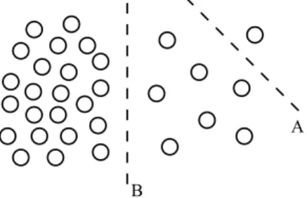
Fig. 1. An example where mincut gives a bad partitionA; we should expect partitionB.
In this paper, a novel spectral clustering method is presented that is based on simple linear algebra techniques. The method reduces the cost by approximating the graph Laplacian by the incomplete Cholesky decomposition with an adaptive stop criterion and has also the possibility to assign new data points to the clusters.
The paper is organized as follows. In Section2, an introduction about spectral clustering is given. In Section 3, a novel spectral clustering algorithm based on linear algebra techniques is proposed. In Section4, the numerical results are presented. Finally, the conclusion is the subject of Section5.
2. Introducing spectral clustering
Because of the overwhelming amount of literature on the subject of spectral clustering, only the main concepts are explained and the reader is referred to [6–9] for more information.
Spectral clustering is a relaxation of a graph partitioning problem that is NP-hard. Hence, we start with introducing a graph. Represent the data points
{x
i}
ni=1as vertices in an undirected graph and assign a positive weightsij, based on asimilarity measure, to the edge betweenxiandxj. From this, a symmetric similarity matrixScan be constructed, i.e., each
element of the matrixSrepresents the similarity between two vertices. The degree of a vertex, which represents the total number of weights of the edges related to a specific vertex, is defined asdi
=
nj=1sij. The degrees of the vertices are
collected in the degree matrix:D
=
diag(
d1, . . . ,
dn)
.The idea of graph clustering is to findksubgraphs such that a minimal number of edges are cut off and that the sum of all weights of these cut edges is minimal. This is called the mincut problem [15] and it results in minimizing:
Cut
(
A1, . . . ,
Ak)
:=
1 2 k
i=1 S(
Ai,
A¯
i),
withS(
A,
A¯
)
:=
i∈A,j∈ ¯ASijand whereA
¯
stands for the complement ofA. A factor 12 is added to avoid counting eachedge twice in the cut. In practice, the method related to this minimization problem does not always result in a satisfactory partition. This is shown inFig. 1, where an individual vertex is isolated (partitionA) instead of the obvious partitionB. The cut value of partitionAis less than the cut value of partitionBbecause for partitionBmore edges must be cut with a higher weight.
To circumvent this, it could be requested that the clustersAi
,
i=
1, . . . ,
kconsist of considerably large groups of datapoints. This can be achieved in two ways; the first way takes the number of vertices in a setAiinto account:
|
Ai|
, and thesecond way takes the weights of the edges in a setAiin consideration: vol
(
Ai)
. Only the second way will be consideredfurther on. This results in minimizing the following objective function [16,6]:
NCut
(
A1, . . . ,
Ak)
:=
1 2 k
i=1 S(
Ai,
A¯
i)
vol(
Ai)
.
(1)This objective function(1)tries to achieve that the clusters are balanced by the corresponding measure. Rewriting the minimization of(1)fork
=
2 results in, [6]:min y yTLy yTDy such thaty
∈ {
1,
−
b}
n,
yTD1 n=
0,
(2)whereL
=
D−
Sis the unnormalized graph Laplacian,yis the discrete indicator vector of lengthncontaining only the values 1 and−
b. The valuebis a positive constant that depends on the number of data points assigned to each partition,b
=
vol(A1) vol(A2).The minimization of(2)is a NP-hard problem. When the discrete condition ofyis relaxed — the values ofycan also take real values (not only 1 and
−
b) — the minimization of(2)results in solving the following eigenvalue problem:D−1Ly
=
λ
y,
(3)withLrw
=
D−1Lthe normalized graph Laplacian.1To obtain an approximated solution of(1), the eigenvectors ofLrw, corresponding to the second smallest eigenvalue (also
called the Fiedler vector) are the real valued solutions to the problem(1). The indicator vector can be obtained by binarizing the Fiedler vector. Hence, the data points are assigned to a cluster based on the corresponding sign of the value in the Fiedler vector.
Generally, when working withkclusters, the problem(1)also reduces to the eigenvalue problem(3). In these cases not only the eigenvector belonging to the second smallest eigenvalue is of interest, but all the eigenvectors corresponding to the 2
, . . . ,
ksmallest eigenvalues. Normally, the eigenspace spanned by the eigenvectors corresponding to theksmallest eigenvalues is taken into account.To obtain the indicator vectors fork
>
2 another clustering algorithm is applied to cluster thekeigenvectors. An example would be thek-means algorithm.Graph Laplacian
Previously, the graph LaplacianL
=
D−
Swas defined. In fact, this is the main tool for spectral clustering and has been extensively investigated in spectral graph theory [7]. We briefly discuss the main properties of three types of graph LaplacianL
,
Lrw,Lsym=
D−1/2LD−1/2=
In−
D−1/2SD−1/2, which are called the unnormalized, the normalized and the symmetricnormalized graph Laplacian, respectively. All three graph Laplacians are positive semi-definite matrices and the matrices
LandLsymare also symmetric. They have the basic property that the smallest eigenvalue is 0 and that the corresponding
eigenvector is the constant one vector1n, except forLsymwhose eigenvector is a scaled version:D1/21n. We consider the
constant vector1nand a multiplea1n, for somea
̸=
0, as the same vectors.A relation also exists between the number of connected components in a graph and the multiplicity of the eigenvalue 0 of the Laplacian.2Before this proposition is defined, the indicator vector1A1should be introduced (we consider the vectors
1A1anda1A1as the same vectors):
(
1A1)
i=
1
,
i∈
A1,
0
,
i̸∈
A1.
Proposition 1. Let G be an undirected graph with nonnegative weights. Then, the multiplicity k of the eigenvalue0of L
,
LrwandLsymequals the number of connected componentsA1
, . . . ,
Akin the graph. For L, Lrw: the eigenspace of eigenvalue0is spannedby the vectors1A1
, . . . ,
1Ak, and for Lsym: the eigenspace of eigenvalue0is spanned by the vectors D 1/21Ai
,
i=
1, . . . ,
k. Proof. See [9].The difference between the unnormalized and normalized Laplacian is that they both take care of minimizing the between-cluster similarity, but only the normalized Laplacian takes care of maximizing the within-cluster similarity. Hence the normalized Laplacian is often chosen.
For more information about the graph Laplacian and other basic properties, the reader is referred to [7,10,11,9]. Note that in the literature no unique convention exists regarding the name graph Laplacian.
3. Clustering algorithm
In this section, a spectral clustering method based on linear algebra techniques is proposed which can be extended to out-of-sample points.
In Section3.1, an approximation of the graph Laplacian is constructed based on a sparse set of data points. The sparse set of data points is obtained using an incomplete Cholesky decomposition with an adapted stopping criterion. In Section3.2, the eigenvalue problem is constructed. In Section3.3, the cluster assignment is explained. In Section3.4, the possibility to extend the method to out-of-sample points is discussed.
3.1. Graph Laplacian
The rationale of this paper is to approximate the positive semi-definite similarity matrixS(which is needed to construct the graph Laplacian) using only a sparse data set such that the approximant captures the structure of the matrix. With the structure of the matrix, the ‘nonzero’ shape of the matrix is meant. Note that it is not the intention to obtain a good approximant in terms of a low rank approximation as often encountered in the literature [17–21], i.e., the norm between the original and the approximated matrix can be large.
Several methods, which construct a low rank approximation of the similarity matrix, exist. In [22] the data points are selected randomly. In [23] the sparse set of data points are called the landmark points, which are the centroids obtained from thek-means clustering algorithm. The clustering problem is then solved for this small subset and this solution is extrapolated to the full set of data points. Randomly selecting the sparse set of data points can lead to wrong clusters, this is shown later on with an example. Using the centroids of thek-means clustering algorithm as the sparse set of data points could be a better option. But the computational complexity related to the acquisition of these centroids is increasing, especially for large scale problems.
2 A connected component is a subgraph in which any two vertices are connected to each other by paths and to which no more vertices or edges can be added while preserving its connectivity.
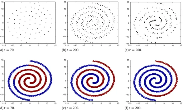
(a) Two clusters. (b) Two spirals.
Fig. 2. Data points(n=1000): (a) two clusters, (b) two spirals.
In [18], the incomplete Cholesky decomposition is used as a low rank approximation assuming that there is a fast decay of eigenvalues. After investigation of the similarity matrices utilized in [18], we noticed that these matrices did not possess this property. This is shown inFigs. 4and5(a), where there is no rapid decay of eigenvalues for the two data sets shown in
Fig. 2. Hence, it is not possible to efficiently approximate the matrix with a matrix of low rank. For that reason we propose the idea about capturing the structure of the matrix using only a sparse data set.
To achieve this, the incomplete Cholesky decomposition with an adapted stopping criterion is introduced. In fact, the incomplete Cholesky decomposition selects the rows and the columns in an appropriate manner such that the structure of the approximation is close to the structure of the original matrix. In other words, the selected rows and columns are related to certain data points, and this sparse set of data points is a good representation of the full data set.
Throughout this paper, the radial basis functionK
(
x,
y)
=
exp
−
∥x−y∥22σ2
with parameter
σ
∈
Ris taken as the similarity measure between two data pointsxandy. In the numerical experiments that work with images, another similarity measure is used, namely theχ
2measure.3.1.1. Cholesky decomposition
A Cholesky decomposition [24] of a matrixA
∈
Rn×nis a decomposition of a symmetric positive definite matrix into theproduct of a lower triangular matrix and its transpose:A
=
CCT, and is widely used for solving linear systems. When the matrixAis positive semi-definite it is possible to compute the incomplete Cholesky decomposition. In fact, the incomplete Cholesky decomposition computes a low rank approximation of accuracyτ
of the matrix inO(
r2n)
such that∥
A−
CCT∥
< τ
withC
∈
Rn×r. As stated in [18], the incomplete Cholesky decomposition leads to small numerical error andr≪
nwhen there is a fast decay of eigenvalues. Algorithm 1 shows the incomplete Cholesky decomposition [25].Algorithm 1Incomplete Cholesky decomposition
1: Puti
=
1,S¯
←
S,P←
In,gj=
Sjjforj=
1, . . . ,
n, 2: while
nj=igj
> τ
do3: Find new pivot elementj∗
=
arg max j∈[i,n]gj.4: Update permutationP:Pii
=
Pj∗j∗=
0 andPij∗=
Pj∗,i=
1.5: Permute elementsiandj∗inS
¯
:S¯
1:n,i
↔ ¯
S1:n,j∗andS¯
i,1:n↔ ¯
Sj∗,1:n.6: Update the already calculated elements ofC:Ci,1:i
↔
Cj∗,1:i.7: SetCii
=
¯
Sii. 8: Calculateithcolumn ofC:Ci+1:n,i=
C1ii
¯
Si+1:n,i−
i−1 j=1Ci+1:n,jCij
.9: Update only diagonal elements: forj
=
i+
1, . . . ,
n:gj=
gj−
Cji2. 10: Seti=
i+
1.11: end while
3.1.2. Ideal situation
To clarify the selection of the incomplete Cholesky decomposition a small example is elaborated. We consider an example with two connected components, i.e., the data points are structured into two disjunct clusters and no connections exist between them. We also assume that the data points are ordered such that the similarity matrixS
∈
Rn×nis a block diagonalmatrix with two blocks
S11,
S22∈
R n 2× n 2
: S=
S11 0 0 S22
.
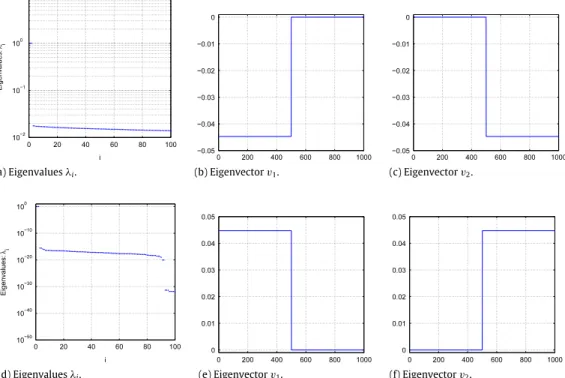
(a) Eigenvaluesλi. (b) Eigenvectorv1. (c) Eigenvectorv2.
(d) Eigenvaluesλi. (e) Eigenvectorv1. (f) Eigenvectorv2.
Fig. 3. Eigenvalues and eigenvectors(n=1000): Block diagonal similarity matrix: (a) eigenvaluesλi, (b) eigenvectorv1, (c) eigenvectorv2. Approximation of block diagonal similarity matrix: (d) eigenvaluesλi, (b) eigenvectorv1, (c) eigenvectorv2.
After two steps of the incomplete Cholesky decomposition algorithm (Algorithm 1), two columnsj∗
=
1 andj∗=
n 2+
1are selected (assuming maximum function selects the first maximum it encounters). These two columns are enough to approximate matrixSin such a way that the structure of matrixSis captured:
S
≈
(
S11)
1:n2,1(
S11)
T1:n2,1 0 0(
S22)
1:n2,1(
S22)
T1:n2,1
.
As can be seen, the approximation ofSconsists of two blocks. This means that the ‘nonzero’ shape of the matrix is the same as the approximationCCT. In fact, the two selected columns
j∗=
1 andj∗=
n2
+
1
are related to a point from another cluster:x1andxn
2+1. Therefore, the structure of the eigenvectors of the approximated graph Laplacian is similar to
the structure of the eigenvectors of the original graph Laplacian.
This is shown inFig. 3for the eigenvalue problemD−1Sy
= ˇ
λ
yfor which the largest eigenvalues become importantinstead of the smallest.3Fig. 3(a) and (d) show the first hundred largest eigenvalues of the matrixSand the matrixCCT, respectively. The two largest eigenvalues are one.Fig. 3(b) and (c) show the eigenvectors
v
1andv
2belonging to the largesttwo eigenvalues for the case where the exact similarity matrixSis used. As one can see, these eigenvectors are1A1and1A2
withA1
=
1, . . . ,
n2
andA2=
n 2+
1, . . . ,
n
. Also the eigenvectors from the approximated caseCCThave this shape
(only alternated), as shown inFig. 3(e) and (f).
3.1.3. Practical case
In practice, the matrixSis not a block diagonal matrix but a permuted version of it and the anti-diagonal blocks also contain information about the data points. An example with two clusters as shown inFig. 2(a) is considered, and the eigenvectors belonging to the two largest eigenvalues for the exact similarity matrix and the one approximated with a rank two matrix (incomplete Cholesky decomposition used for selection) are investigated. Assume that the data points are still ordered such that the eigenvectors can be clearly visualized.
In the first row ofFig. 4, the results for the eigenproblem solved with the exact similarity matrix are shown. As one can see, inFig. 4(a) there is no fast decay of eigenvalues. InFig. 4(b), the eigenvector
v
1belonging to the largest eigenvalue isa constant eigenvector1n, and inFig. 4(c), the eigenvector
v
2belonging to the second largest eigenvalue nicely indicatesthe clusters (binarizing would give the clusters). This is also the case when the eigenproblem is solved with the rank two approximation of the similarity matrix. This is shown in the second row ofFig. 4.
(a) Eigenvaluesλi. (b) Eigenvectorv1. (c) Eigenvectorv2.
(d) Eigenvaluesλi. (e) Eigenvectorv1. (f) Eigenvectorv2.
Fig. 4. Eigenvalues and eigenvectors for two clusters(n=1000, σ=0.4). Exact similarity matrix: (a) eigenvaluesλi, (b) eigenvectorv1, (c) eigenvector
v2. Approximation of similarity matrix: (d) eigenvaluesλi, (e) eigenvectorv1, (f) eigenvectorv2.
Note that the constant vector (eigenvector
v
1) inFig. 4(b) and (e) does not look like a straight line but has the same shapeas the eigenvector
v
2. The figure indicates that there is a small jump around 500, but only a small change in they-value.Probably, the structure of the eigenvector is intrinsically available in this vector.
3.1.4. Practical case: intermingled clusters
There exist examples of two clusters where computing a rank two approximation of the similarity matrix is not satisfactory. For instance, in the example with the two intermingled spirals shown inFig. 2(b). The distances between points in different clusters can be smaller than between points in the same cluster. This information is also incorporated in the similarity matrixS. For this type of example, it will not work to select two pivots, each from a different cluster, and solve the corresponding eigenvalue problem. In fact, more pivots must be selected. This is shown inFig. 5.
Fig. 5(a) shows that there is no fast decay of eigenvalues andFig. 5(b) and (c) gives the eigenvectors belonging to the largest two eigenvalues, when the exact similarity matrix is used. The first eigenvector
v
1is the constant eigenvector andthe second eigenvector
v
2shows nicely the two clusters. The results of the eigenproblem where the similarity matrix isapproximated with a rank 100 matrix are shown in the second row ofFig. 5. The two eigenvectors belonging to the two largest eigenvalues are shown: the first eigenvector
v
1is the constant vector and the second eigenvectorv
2clearly indicatesthe two clusters.
When an approximation of a rank 70 matrix is used instead of a rank 100 approximation, the method does not work. Additionally, when selecting the pivots arbitrarily and not according to the selection procedure of the incomplete Cholesky decomposition this is also the case. This is shown inFig. 6. A correct clustering is obtained when a minimal number of pivots is selected so that the clusters are visually noticeable, which is only the case inFig. 6(d).
Notice that the sparse set of data points related to the selected pivots of the incomplete Cholesky are located at a certain distance from each other, seeFig. 6(a) and (c). This depends on the radial basis function parameter
σ
. A largerσ
will result in data points which are further away from each other, such that the data set is sparse but not a good representation of the full data set. A smallerσ
results in data points that are closer to each other, such that more pivots are selected to obtain the correct clustering. The selection of the parameterσ
will not be a topic of this paper, but one of future research.3.1.5. Stopping criterion
As shown above, the incomplete Cholesky decomposition selects the pivots in such a way that a sparse representation of the data set is obtained. In the next step the stopping criterion of the decomposition is adapted, it is no longer based on the idea of a low rank approximation (Algorithm 1), because these matrices do not possess this property. We want the algorithm to stop when a minimal number of data points is selected, which ensures a correct clustering.
(a) Eigenvaluesλi. (b) Eigenvectorv1. (c) Eigenvectorv2.
(d) E igenvaluesλi. (e) Eigenvectorv1. (f) Eigenvectorv2.
Fig. 5. Eigenvalues and eigenvectors for two spirals(n=1000, σ=0.5). Exact similarity matrix: (a) eigenvaluesλi, (b) eigenvectorv1, (c) eigenvector
v2. Approximation of similarity matrix: (d) eigenvaluesλi, (e) eigenvectorv1, (f) eigenvectorv2.
(a)r=70. (b)r=200. (c)r=200.
(d)r=70. (e)r=200. (f)r=200.
Fig. 6. Data point related to the selected pivots(r)and the resulting clusters(n=1000, σ =0.5): (a)–(d) selection based on the incomplete Cholesky decompositionr=70, (b)–(e) selection based on the incomplete Cholesky decompositionr=200, (c)–(f) random selection of pivotsr=200.
The stopping criterion is based on the degree of each vertex in the approximation of the similarity matrixS. As defined before, the degree of a vertex,dj, represents all the connections to the other vertices, i.e. the sum of all weights of the
edges connected to the vertex. When the matrixSis approximated, the degree matrix is also approximated. Therefore an approximation of the degreed
˜
jis used in this stopping criterion. Because a sparse set of data points is selected iterativelyin the incomplete Cholesky decomposition, only the connections of the vertices to the points related to the selected data points can be taken into account, i.e., it corresponds to diag
(
D˜
)
=
CCT1n.In fact, each vertex must have a certain degree to ensure a good clustering. This means that there must be enough connections to the vertices related to the already selected data points. If there is still a vertex with degree zero, a new pivot should be selected. After the selection of a new pivot, the degrees of the vertices are updated and based on these values the stopping criterion is verified. It is found that the following stopping condition
mind
˜
jmaxd
˜
j>
10−3 (4)gives satisfactory results. This means that each vertex has a certain degree related to the already selected data points. Probably there exist cases where the bound can be chosen less or more severe, but from our experience this bound gives satisfactory results. This will be further discussed in the numerical experiments of Section4.
3.2. Reducing the size of the eigenvalue problem
In this section, the reduction to a smaller eigenvalue problem is clarified. It is similar to the method proposed in [18]. In this paper we are mainly interested in solving the following eigenvalue problem:
ˆ
Lsymy
= ˆ
λ
y withLˆ
sym=
D−1/2SD−1/2.
Notice that the eigenvalues ofL
ˆ
symare related to those ofLsymasλ
ˆ
=
1−
λ
. Hence, the largest eigenvalues become importantinstead of the smallest. In Section3.1, the incomplete Cholesky decomposition ofSis defined asS
≈
CCT, withC∈
Rn×r
andrthe number of selected pivots. Substituting this, together with the related degree matrixD
˜
, inLˆ
symresults in:ˆ
Lsym
≈ ˜
D−1/2CCTD˜
−1/2.
(5)To reduce the size of the eigenvalue problem, replaceD
˜
−1/2Cwith itsQRdecompositionD˜
−1/2C=
QR, whereQ∈
Rn×r,andR
∈
Rr×r and substituteRwith its singular value decompositionR=
URΣRVRT, whereUR
,
VR∈
Rr×r andΣR∈
Rr×r.Eq.(5)results in:
ˆ
Lsym
≈
(
QR)(
QR)
T≈
Q(
URΣRVRT)(
VRΣRURT)
QT≈
QUR(
ΣR)
2URTQ T.
The columns of the matrixV
˜
=
QUR,1:kwithV˜
∈
Rn×kare thekorthogonal eigenvectorsv˜
jwith respect to thekdominanteigenvalues
(σ
R,j)
2= ˜
λ
jwithj=
1, . . . ,
k.3.3. Cluster assignment
To explain the cluster assignment, the case ofkconnected components, with thekdominant eigenvalues
λ
˜
1= · · · =
˜
λ
k=
1 and the corresponding eigenvectorsv˜
j,
j=
1, . . . ,
k, is considered. According toProposition 1, the followingdecomposition holds:
˜
D−1/2
[˜
v1. . .
v˜
k] = [1
A1. . .
1Ak]
DIQI,
whereDI
∈
Rk×kis the matrix containing the scaling parameters andQI∈
Rk×ka unitary matrix. Extraction of the indicatorvectors from thekeigenvectors can be achieved by computing a pivotedLQdecomposition of the eigenvector matrixD
˜
−1/2V˜
, as proposed in [26]:˜
D−1/2V˜
=
PLQV˜=
P
L11 L22
QV˜,
withP
∈
Rn×na permutation matrix,L11∈
Rk×klower triangular matrix,L22∈
R(n−k)×kandQV˜∈
Rk×kan unitary matrix.Put
ˆ
L=
L11 L22
L−111=
Ik L22L−111
.
Then the columns ofY
=
Pˆ
Lare the indicator vectors:Y
= [1
A1. . .
1Ak]
.
In fact, the underlying process of theLQ factorization of a matrixA
∈
Rn×kcan be explained with the Gram–Schmidt process [24]. Different pointsxibelonging to clusterjwill be selected, these points will be the representatives of the clusterj. In fact, for each cluster the algorithm selects a representative. Then the entries of matrixL
ˆ
give an indication of how a point is related to a certain cluster.In practice, when there are almostk connected components, the cluster structure is still inherited but the zeros in
1Al
(
l=
1, . . . ,
k)
become real values different from zero. The magnitude (in absolute value) of the entries,yij, of the matrixY
=
Pˆ
L∈
Rn×kindicate how well a data pointxiis assigned to clusterj. Then, a data pointxican be assigned to a clusterjwhen
j
=
arg maxl
(
|
(
Y)
i,l|
).
Hence, the matrixY also gives a measure of how well or poorly a data point belongs to a certain cluster based on thek
representatives. This measure could be used to detect outliers in the data.
Because the proposed algorithm is based on the approximation of the similarity matrixS, the correct information of only a sparse set of data points related to the selected pivots is exploited; the information of the other points is approximated. To take this into consideration in the cluster assignment, the eigenvectorsV
˜
are scaled with the degree matrixD˜
1/2such that if the approximated degree of a vertex is small, this point will not be selected as a representative of a cluster. This corresponds to the operationD˜
(
D˜
−1/2V˜
)
on the eigenvectors.3.4. Generalization to out-of-sample points
When working with data sets it occurs that new data points (also called out-of-sample points) appear, which also must be assigned to a cluster. To circumvent the recomputation of an eigenvalue problem of larger size, a method using only the information related to the selected pivots (obtained in the previous sections) is proposed. Hence, the out-of-sample points
{x
i}
ni=out1 can be assigned to a cluster.This is achieved by relating the out-of-sample points
{x
i}
ni=out1 to the sparse set of data points{x
i}
ri=1 (selected by theincomplete Cholesky decomposition). In fact, we compute sequentiallyCext
,
Qext,V˜
extandYextbased on information fromthe clustering algorithm. In the following formulae, the original steps of the clustering algorithm (on the left) are shown together with the steps which must be executed to cluster the out-of-sample points (on the right).
In the first step, the approximation of the similarity matrix between the out-of-sample points
{x
i}
ni=out1and the data points{ ˜
xi}
ri=1related to the selected pivots is computed:S
=
CCT→
Sext=
C Cext
CT CextT
,
whereCext
∈
Rnout×r. Notice that we only compute the entries related to therselected data points obtained with theincomplete Cholesky decomposition (Algorithm 1 with adapted stopping criterion) and not related to thendata points. The second step is to compute an extended version of the eigenvectors; instead of recomputing the eigenvector matrix of size
(
n+
nout)
×
k, only the bottomnoutrows are computed. This computation is based on information from the originaldecomposition andCext. First, the matrixQextis computed based on information of theQRdecomposition ofD
˜
−1/2C:˜
D−1/2C
=
QR→
Qext= ˜
D −1/2 ext CextR−1,
withQext
∈
Rnout×r and diag(
D˜
ext)
=
CextCextT 1nout. Then, the information of the eigenvectorsUR,1:kis applied to obtain thenew rows of the eigenvector matrixV
˜
ext∈
Rnout×k.˜
V
=
QUR,1:k→ ˜
Vext=
QextUR,1:k.
When the extension of the eigenvector matrix,V
˜
ext, is obtained these rows must be transformed in the same way as allprevious rows of the eigenvector matrix, as in Section3.3, to obtain the cluster assignments. This is done by applyingQ˜T
V
toV
˜
ext:˜
DV˜V
˜
=
YQV˜→
Yext= ˜
DV˜extV˜
extQV˜T,
withYext
∈
Rnout×k. Then, the same cluster assignment criterion can be used to assign the out-of-sample pointxito a cluster:assign pointxito clusterjwhen
j
=
arg maxl
(
|
(
Yext)
i,l|
).
3.5. Algorithm
An overview of the method is given in Algorithm 2.
Note:The proposed method has a few similarities to the method proposed by Alzate and Suykens in [18], like the use of the incomplete Cholesky decomposition and the reduction to a smaller eigenvalue problem. But there are also significant differences. The method proposed by these authors is based on a kernel principal component formulation and leads to the
Algorithm 2Sparse model for spectral clustering using the incomplete Cholesky decomposition
1: Compute the incomplete Cholesky factorC
∈
Rn×rof the matrixSsuch that matrixCCTcaptures the structure of matrixSand obtain the sparse setR
= { ˜
xi}
ri=1of pivots.2: Compute theQRdecomposition ofD
˜
−1/2C=
QRwithQ∈
Rn×randR
∈
Rr×r.3: Compute the singular value decomposition ofR
=
UΣVT. 4: Obtain the approximated eigenvectors via:V˜
=
QUR,1:k.5: ComputeLQfactorization with row pivotingDV˜V
˜
=
PLQV˜ and putY=
PLˆ
withˆ
L=
LT 11 LT22
TL−111.
6: For alli, assign pointxito clusterjwhenj
=
arg maxl(
|
Yi,l|
)
. 7: ComputeCext∈
Rnout×r.8: ComputeQext
= ˜
D −1/2ext CextR−1andV
˜
ext=
QextURand putYext=
DV˜extV˜
extQVT˜. 9: For alli, assign pointxito clusterjwithj=
arg maxl(
|
(
Yext)
i,l|
)
.following eigenvalue problem:
MSy
=
λ
y (6)withM
=
D−1−
11TnD−11n
D−11 n1TnD
−1a weighted centering matrix removing the weighted mean from each column of the
matrixS. Another difference is that the incomplete Cholesky decomposition with the original stopping criterion is used. This results in an extra parameter in their spectral clustering algorithm, which has to be chosen in a proper way.
4. Numerical experiments
In this section, the proposed method (FV, abbreviation for Frederix-Van Barel) is compared with the method of Alzate and Suykens (AS) [18] on different problems. Because the methodASdepends on an extra parameter
τ
, we compare the results with an adapted version of the method ofAS, which is denoted by methodAS(*). In this method, the number of pivots is given as input such that the methodFVand methodAS(*) have the same number of pivots.The first experiment shows that the methodFVis based on a sparse set of data points and it also shows the idea behind the stopping condition(4)for two different problems. The second experiment shows the results concerning the out-of-sample extensions for three different problems. The third experiment shows the use of the algorithm for image segmentation.
In the first experiment, the whole data set is considered as one set (also called the training set) and in the second experiment, the data set is divided into two sets, the training set and the out-of-sample set. The results are compared with a known clustering. This is done using the adjusted rand index (ARI) [27], which measures the similarity between two data clusterings. The adjusted rand index has a value between 0 and 1, with 0 indicating that the two data clusters do not agree on any pair of points and 1 indicating that the data clusters are exactly the same. The simulations are performed ten times, so average results are shown in the figures and tables.
Experiment1. Sparseness obtained by methodFV.
Three Gaussian clouds in3D: InFig. 7(a) the three clouds are shown. The number of training points isn
=
6000 and the radial basis function parameterσ
is fixed toσ
=
3. InFig. 7(b), the stopping criterion(4)on a logarithmic scale for the first 100 selected pivots of the methodFVis shown. It gives the value(4)after each selection of a new pivot. As one can see, the stopping criterion is fulfilled when three pivots are selected, and a correct clustering is obtained. Notice that the bound of the stopping criterion could have been 10−2, this would give the same result.In this experiment, the effect of the parameter
τ (
10−5≤
τ
≤
1)
of methodASis compared to the methodFVthat does not have an extra parameter. InFig. 7(c), the number of selected pivots is shown for the two methods. The methodFVdoes not depend on the parameter
τ
, so its result stays fixed (dotted line). For the methodASthe number of selected pivots decreases whenτ
increases. Forτ
close to one, the same number of pivots is selected as in the methodFV.For the last value of
τ,
2.
2 data points (not an integer because of the randomization) are selected, which is even smaller than the value of the methodFV. In this case the adjusted rand index does not give 1 but 0.6138, so no correct clustering is obtained. In fact, for three clouds at least three pivots must be selected to obtain a correct clustering. InFig. 7(d) the computation times in seconds are shown, which decreases also whenτ
increases for methodASbut it is higher than the computation time of the methodFV.Two spirals in2D: In this experiment two spirals are considered, as shown inFig. 8(c). First, we considern
=
1000 data points and the radial basis function kernel parameter is set toσ
=
0.
4. InFig. 8(a) and (b) the stopping criterion(4)is shown with respect to the number of selected pivots.Fig. 8(a) gives the behavior of the stopping condition(4), andFig. 8(b) gives the result in a specific interval[
50,
200]
. The red dot indicates that from this point on a correct clustering (ARI=
1) is obtained. Notice that at that moment the stopping criterion is not fulfilled, but that we could have put the bound of the stopping criterion to 10−5to obtain the same clustering. Putting the bound to 10−2, as mentioned in the previous experiment with the three Gaussian clouds, would lead to a larger, which is not preferable. InFig. 8(c) the data points related to the selected pivots are shown, the dots denote the ones that are sufficient to obtain the correct clustering, the plus signs are the data points that are selected until the stopping condition is fulfilled.(a) Clusters. (b) Stopping condition.
(c) Pivots. (d) Time.
Fig. 7. Experiment 1: Three Gaussian clouds(n=6000, σ=3): (a) clustering obtained with methodFV, (b) stopping criterion(4)for the first 100 selected pivots, (c) number of selected pivots, (d) computation time (in seconds).
(a) Stopping condition. (b) Close up stopping condition. (c) Clusters.
Fig. 8. Experiment 1: Two spirals(n=1000, σ=0.4): (a) stopping criterion(4)for the first 300 selected pivots, (b) close-up of stopping criterion(4), (c) clustering obtained with methodFV, the data points related to the selected pivots are marked.
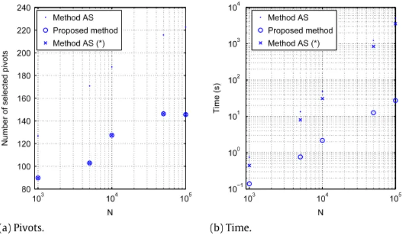
InFig. 9(a) and (b), the number of selected pivots and the computation times are shown for increasingnand
τ
=
0.
7. As one can see, the methodFVselects fewer pivots, and the computation times reduce significantly. Also in comparison with methodAS(*) the reduction time is significant. Note that the full approach does not fit into memory. The valueτ
=
0.
7 is a good choice for the methodAS, taking another value forτ
is not going to reduce the computational time drastically. In fact, methodAS(*) is a method related to another value ofτ
, and there is no extreme decrease in the computational complexity. InTable 1, the number of selected pivots is shown for the methodASand the methodFV. Also the degree of sparseness is indicated.Experiment2. Out-of-sample extensions.
Three Gaussian clouds in2D: In this experiment, the effect of the number of training points is investigated on an almost ideal problem (clusters well separable) and on a non-ideal problem (clusters hard to separate), seeFigs. 10(a) and11(a). The number of data points isn
=
900, the radial basis function parameterσ
is set to 0.8 and 0.5 respectively, andτ
is 0.5 in(a) Pivots. (b) Time.
Fig. 9. Experiment 1: Two spirals(σ=0.4, τ=0.7): (a) number of selected pivots with respect ton, (b) computation times with respect ton.
Table 1
Experiment 1: Two spirals: number of selected pivotsrwith respect tonfor methodASand methodFV. The percentage indicates the degree of sparseness.
Sizen Pivots MethodAS Pivots methodFV
1 000 129 (87.1%) 94 (90.6%)
5 000 169 (96.6%) 100 (98.0%) 10 000 186 (98.1%) 121 (98.8%) 50 000 216 (99.6%) 143 (99.7%) 100 000 224 (99.8%) 144 (99.9%)
both cases. The number of training points varies fromntrain
=
20, . . . ,
880 with steps of 20, and the remaining data pointsare attributed to the out-of-sample set.
Fig. 10(b)–(d) shows the number of selected pivots, the computation times in seconds and the adjusted rand index for increasing number of training points.Fig. 10(b) shows that if more training points are selected the number of selected pivots increases. The increase is stronger for methodASthan for the methodFV. Maybe we should vary
τ
whenntrainis increasing.InFig. 10(c) it is shown that if the number of pivots increases, the computation times also increase.Fig. 10(d) shows the adjusted rand index. MethodFVgives a correct clustering immediately, while methodASneeds one step more to obtain a correct clustering.
InFig. 11(a), the three clouds are not well defined: they are visually distinguishable but there are several points that are hard to assign to a specific cluster.Fig. 11(b) shows that, if more training points are selected, more pivots will be selected. This also gives an increase in the computation times (Fig. 11(c)).Fig. 11(d) shows the adjusted rank index, this index is slightly better for methodASthan for the methodFV. This is probably the case because the methodASselects more pivots than the methodFV. When methodFVis compared to methodAS(*), it is revealed that in most cases the methodFVobtains a slightly better adjusted rand index.
k Gaussian clouds in2D with k
=
2, . . . ,
10: In this experiment the effect of an increasing number of clusters for a fixed number of training points is investigated. The dataset containsn=
2000 data points, of which one fifth are used for training and the remaining points for testing. The radial basis function parameterσ
is fixed toσ
=
0.
5, andτ
=
0.
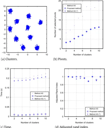
5.Fig. 12(a) shows the data points for ten clusters.Fig. 12(b)–(d) shows the number of selected pivots, the computation time and the adjusted rand index for an increasing number of clusters. The methodFVselects fewer pivots than method
AS. The adjusted rand index indicates that the methodFVis comparable with methodAS, and performs slightly better than methodAS(*) for an increasing number of clusters.
Three concentric rings in a2D space: In this experiment, a nonlinear problem where the data points have few members and the rings have a multiscale nature, is investigated. InFig. 13the concentric rings are shown.Table 2shows the results for an optimal and a non-optimal
σ
: 0.1 and 0.2 respectively. The data set consists ofn=
1400 points, of which 600 points are used for training(
ntrain)
and the other 800 for testing(
nout)
. The methods have a similar behavior, because almost the samenumber of pivots are selected. The methodFVgives a slightly better result.
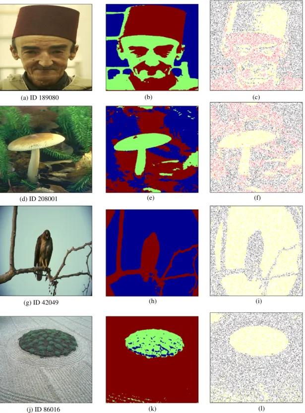
Experiment3: Image segmentation
This experiment shows the use of the proposed algorithm for image segmentation. Therefore we use some of the color images from the Berkeley image dataset4[28]. A local color histogram with a 5
×
5 pixels window around each pixel usingminimum variance color quantization of 8 levels is used. To compute the distance between two local color histogramsh(i)
(a) Clusters. (b) Pivots.
(c) Time. (d) ARI.
Fig. 10. Experiment 2: Three Gaussian clouds in 2D(n = 900, σ = 0.8, τ = 0.5): (a) three clusters, (b) number of selected pivots in training set, (c) computation time (in seconds), (d) adjusted rand index.
(a) Clusters. (b) Pivots.
(c) Time. (d) ARI.
Fig. 11. Experiment 2: Three Gaussian clouds in 2D(n=900, σ=0.5, τ=0.5): (a) clusters, (b) number of selected pivots in training set, (c) computation time (in seconds), (d) adjusted rand index.
(a) Clusters. (b) Pivots.
(c) Time. (d) Adjusted rand index.
Fig. 12. Experiment 2:kclusters withk=2, . . . ,10 in 2Dspace with varying number of training points(n=2000, σ=0.5, τ=0.5): (a) ten clusters, (b) number of selected pivots in training set, (c) computation time (in seconds), (d) adjusted rand index.
Fig. 13. Experiment 2: Three concentric rings in 2Dspace for an optimalσ=0.1 and a non-optimalσ=0.2(n=1400, τ=0.65).
Table 2
Experiment 2: Three concentric rings in a 2Dspace: results for an optimalσ = 0.1 and a non-optimal
σ=0.2(n=1400, τ=0.65).
Optimalσ=0.1 Non-optimalσ=0.2
Pivots Time (s) ARI Pivots Time (s) ARI MethodAS 93 0.5203 0.8526 45 0.2109 0.4778 MethodFV 87 0.2242 0.8693 42 0.0429 0.4852 MethodAS(*) 87 0.4698 0.8547 42 0.2036 0.4828
andh(j)the
χ
2-test is used [29]:χ
2 ij=
0.
5
L l=1(
h (i) l−
h (j) l)
2/(
h (i) l+
h (j)l
)
, whereLis the total number of quantizationlevels. We assume that the histograms are normalized
L l=1h(i)
l
=
1,
i=
1, . . . ,
n. To compare the similarity betweentwo histograms for color discrimination and image segmentation in an efficient way, the positive definite
χ
2-kernel,(a) ID 189080 (d) ID 208001 (g) ID 42049 (j) ID 86016 (b) (c) (f) (e) (h) (i) (l) (k)
Fig. 14. Experiment 3: Image segmentation: (a) original image, (b) segmented image, (c) out-of-sample image.
Four different images from the Berkeley image dataset are considered
(
n=
154 401)
. Note that the full problem does not fit into memory. The parameterσ
χis fixed to 0.
25 for each image. The first two columns ofTable 3gives the number of clusterskand the number of selected pivots,r, in the incomplete Cholesky decomposition.Fig. 14gives the resulting images for these values (the original, and the segmented images). As one can see, these images give a good visualization of the original images. In fact, onlyrdata points (seeTable 3) out of 154 401 are selected to obtain these results.Table 3
Experiment 3: Image segmentation. The number of clusterskand the number of selected pivotsrin the incomplete Cholesky decomposition for (a) four images and (b) four images for a training set of 1000 points (Out-of-sample experment).
k r k r
ID 189080 3 27 3 22
ID 208001 3 19 3 19
ID 42049 2 73 2 29
ID 86016 3 18 3 14
InFig. 14(f), the branches and the bird are clearly visible from the background. But notice that the corners of the image are not clustered in the same cluster as the background. At first sight, a person would not make this distinction, but when looking closer at the original image, the difference in background colors is noticeable.
Also some experiments for out-of-sample points are executed. From the data points
(
n=
154 401)
, 1000 training points are selected randomly on which the clustering algorithm is applied. Then 20 000 out-of-sample points are randomly selected from the remaining points, and these points are clustered based on information of the clustering algorithm. The parameterσ
χis fixed to 0.25 for each image.The two right columns ofTable 3give the number of clusterskand pivotsrfor the clustering algorithm for the 1000 training data points.Fig. 14(third column) shows the results of clustering the 20 000 out-of-sample points with the extension of the clustering algorithm. It shows that the main objects of the images are visible and that it gives a nice indication of the shape of the image.
5. Conclusion
A sparse spectral clustering method that is based on linear algebra techniques is presented. In fact, the data set is represented with only a sparse set of pivots, and based on this information the indicator vectors are derived. To achieve this, an adapted stopping criterion for the incomplete Cholesky decomposition is proposed such that no extra parameter is necessary in the algorithm. The proposed method is also extended to out-of-sample points. In the numerical simulations, it is shown that the presented method achieves good results compared to methodAS[18], especially when looking at the computational complexity.
Acknowledgments
The research was partially supported by the Research Council K.U.Leuven, project OT/00/16 (SLAP: Structured Linear Algebra Package), OT/05/40 (Large rank structured matrix computations), OT/10/038 (Multi-parameter model order reduction and its applications), CoE EF/05/006 Optimization in Engineering (OPTEC), PF/10/002 Optimization in Engineering Centre (OPTEC), by the Fund for Scientific Research–Flanders (Belgium), projects G.0078.01 (SMA: Structured Matrices and their Applications), G.0176.02 (ANCILA: Asymptotic aNalysis of the Convergence behavior of Iterative methods in numerical Linear Algebra), G.0184.02 (CORFU: Constructive study of Orthogonal Functions) G.0455.0 (RHPH: Riemann–Hilbert problems, random matrices and Padé–Hermite approximation), G.0423.05 (RAM: Rational modelling: optimal conditioning and stable algorithms), and by the Interuniversity Attraction Poles Programme, initiated by the Belgian State, Science Policy Office, Belgian Network DYSCO (Dynamical Systems, Control, and Optimization). The scientific responsibility rests with its authors.
References
[1] G.H. Ball, D.J. Hall, ISODATA: a novel method of data analysis and pattern recognition. Technical report, Stanford Research Institute, Menlo Park, CA, 1965.
[2] G.H. Ball, D.J. Hall, A clustering technique for summarizing multi-variate data, Behavioral Science 12 (1967) 153–156. [3] R.O. Duda, P.E. Hart, D.G. Stork, Pattern Classification, John Wiley, New York, 2001.
[4] D. Hand, H. Mannila, P. Smyth, Principles of Data Mining, MIT Press, Cambridge, MA, 2001. [5] S. Theodoridis, K. Koutroumbas, Pattern Recognition, Academis Press, San Diego, CA, 2003.
[6] J. Shi, J. Malik, Normalized cuts and image segmentation, IEEE Transactions on Pattern Analysis and Machine Intelligence 22 (8) (2000) 888–905. [7] F. Chung, Spectral Graph Theory, American Mathematical Society, 1997.
[8] A. Ng, M. Jordan, Y. Weiss, On spectral clustering: analysis and an algorithm, in: Advances in Neural Information Processing Systems, vol. 14, 2002. [9] U. von Luxburg, A tutorial on spectral clustering, Statistics and Computing 17 (2007) 395–416.
[10] B. Mohar, The Laplacian spectrum of graphs, in: Graph Theory, Combinatorics, and Applications, vol. 2, 1991, pp. 871–898.
[11] B. Mohar, Some applications of Laplace eigenvalues of graphs, in: G. Hahn, G. Sabidussi (Eds.), Graph Symmetry: Algebraic Methods and Applications, vol. 497, Kluwer, 1997, pp. 225–275.
[12] Y. Bengio, J.-F. Paiement, P. Vincent, O. Delalleau, J. Le Roux, M. Ouimet, Out-of-sample extensions for LLE, isomap, MDS, eigenmaps, and spectral clustering, in: Advances in Neural Information Processing Systems, 2004.
[13] C. Alzate, J. Suykens, A weighted kernel PCA formulation with out-of-sample extensions for spectral clustering methods, in: Proceedings of the 2006 International Joint Conference on Neural Networks, 2006, pp. 138–144.
[14] C. Alzate, J. Suykens, Multiway spectral clustering with out-of-sample extensions through weighted kernel PCA, IEEE Transactions on Pattern Analysis and Machine Intelligence 32 (2) (2010) 335–347.
[15] M. Stoer, F. Wagner, A simple min-cut algorithm, Journal Association for Computing Machinery 44 (4) (1997) 585–591.
[16] L. Hagen, A. Kahng, New spectral methods for ratio cut partitioning and clustering, IEEE Transactions on Computer-Aided Design 11 (9) (1992) 1074–1085.
[17] S. Fine, K. Scheinberg, Efficient SVM training using low-rank kernel representations, Journal of Machine Learning Research 2 (2001) 243–264. [18] C. Alzate, J. Suykens, Sparse kernel models for spectral clustering using the incomplete Cholesky decomposition, in: Proceedings of the 2008
International Joint Conference on Neural Networks, June 2008, pp. 3555–3562.
[19] C. Alzate, J. Suykens, A regularized kernel CCA contrast function for ICA, Neural Networks 21 (2–3) (2008) 170–181. Special issue on advances in neural networks research.
[20] A. Gretton, R. Herbrich, A. Smola, O. Bousquet, B. Schölkopf, Kernel methods for measuring independence, Journal of Machine Learning Research 6 (2005) 2075–2129.
[21] C. Alzate, J. Suykens, ICA through an LS-SVM based kernel CCA measure for independence, in: Proceedings of the 2007 International Joint Conference on Neural Networks, 2007, pp. 2920–2925.
[22] C. Fowlkes, S. Belongie, F. Chung, J. Malik, Spectral grouping using the Nyström method, IEEE Transactions on Pattern Analysis and Machine Intelligence 26 (2) (2004).
[23] K. Zhang, I. Tsang, J. Kwok, Improved Nyström low-rank approximation and error analysis, in: Proceedings of the 25th International Conference on Machine Learning, 2008, pp. 273–297.
[24] G.H. Golub, C.F. Van Loan, Matrix Computations, third ed., Johns Hopkins University Press, Baltimore, Maryland, USA, 1996. [25] F. Bach, M. Jordan, Kernel independent component analysis, Journal of Machine Learning Research 3 (2002) 1–48.
[26] H. Zha, C. Ding, M. Gu, X. He, H. Simon, Spectral relaxation fork-means clustering, in: Advances in Neural Information Processing Systems, 2002, pp. 1057–1064.
[27] L. Hubert, P. Arabie, Comparing partitions, Journal of Classification 2 (1) (1985) 193–218.
[28] D. Martin, C. Fowlkes, D. Tal, J. Malik, A database of human segmented natural images and its application to evaluating segmentation algorithms and measuring ecological statistics, in: 8th International Conference Computer Vision, vol. 2, 2001, pp. 416–423.
[29] J. Puzicha, T. Hofmann, J. Buhmann, Non-parametric similarity measures for unsupervised texture segmentation and image retrieval, Computer Vision and Pattern Recognition (1997) 267–272.