A Dissertation by
YOUTING SUN
Submitted to the Office of Graduate Studies of Texas A&M University
in partial fulfillment of the requirements for the degree of DOCTOR OF PHILOSOPHY
May 2012
A Dissertation by
YOUTING SUN
Submitted to the Office of Graduate Studies of Texas A&M University
in partial fulfillment of the requirements for the degree of DOCTOR OF PHILOSOPHY
Approved by:
Co-Chairs of Committee, Edward R. Dougherty Ulisses Braga-Neto Committee Members, Aniruddha Datta
Ivan Ivanov
Head of Department, Costas Georghiades
May 2012
ABSTRACT
Model-based Biomarker Detection and Systematic Analysis in Translational Science. (May 2012)
Youting Sun, B.S., Tsinghua University
Co–Chairs of Advisory Committee: Dr. Edward R. Dougherty Dr. Ulisses Braga-Neto
This dissertation is concerned with the application of mathematical modeling and statistical signal processing into the rapidly expanding fields of proteomics and genomics. The research is guided by a translational goal which drives the problem formalization and experimental design, and leads to optimization, prediction and con-trol of the underlying system. The dissertation is comprised of three interconnected subjects.
In the first part of the dissertation, two Bayesian peptide detection algorithms are proposed to optimize the feature extraction step, which is the most fundamental step in mass spectrometry-based proteomics. The algorithms are designed to tackle data processing challenges that are not satisfactorily addressed by existing methods. In contrast to most existing methods, the proposed algorithms perform deisotoping and deconvolution of mass spectra simultaneously, which enables better identification of weak peptide signals. Unlike greedy template-matching algorithms, the proposed methods have the capability to handle complex spectra where features overlap. The proposed methods achieve better sensitivity and accuracy compared to many popular software packages such as msInspect.
In the second part of the dissertation, we consider modeling and assessing the entire mass spectrometry-based proteomic data analysis pipeline. Different modules
are identified and analyzed, resulting in a framework that captures key factors in sys-tem performance. The effects of various model parameters on protein identification rates and quantification errors, differential expression results, and classification per-formance are examined. The proposed pipeline model can be used to aid experimental design, pinpoint critical bottlenecks, optimize the workflow, and predict biomarker discovery results.
Finally, the same system methodology is extended to analyze the workflow in DNA microarray experiments. A model-based approach is developed to explore the relationship among microarray data properties, missing value imputation, and sam-ple classification in a complicated data analysis pipeline. The situations when it is suitable to apply missing value imputation are identified and recommendations re-garding imputation are provided. In addition, a missing value rate-related peaking phenomenon is uncovered.
ACKNOWLEDGMENTS
I would like to gratefully acknowledge my advisor, Dr. Edward R. Dougherty, whose constant support creates an ideal environment for my doctoral research. His experienced insights shed light on my intellectual development, career path and be-yond.
I am also deeply indebted to my co-adviser, Dr. Ulisses Braga-Neto, without whose sincere care and guidance the work would not have been possible. His wit and passion towards research and his dedication to students inspired me throughout the years.
I would also like to thank other fine scientists on my committee, Dr. Aniruddha Datta and Dr. Ivan Ivanov, for their constructive advice. I am grateful to my collaborator Dr. Jianqiu Zhang for many stimulating and helpful discussions, to my colleagues and friends Dr. Jianping Hua, Dr. Golnaz Vahedi, and Dr. Jian Liu for their generous help.
Finally, I would like to thank my parents for their great vision and guidance, endless love and support.
TABLE OF CONTENTS
CHAPTER Page
I INTRODUCTION. . . 1
A. MS-based proteomics . . . 2
1. Feature extraction in MS data analysis . . . 4
2. MS analysis pipeline for biomarker discovery . . . 6
B. DNA microarray-based genomics . . . 7
C. Organization of the dissertation . . . 7
D. Main contributions . . . 9
II BAYESIAN PEPTIDE DETECTION FOR MASS SPEC-TROMETRY . . . 11
A. Background . . . 11
B. Methods . . . 12
1. Spectrum preprocessing and obtaining peptide candidates 13 2. Modeling the mass spectrum . . . 14
3. Bayesian peptide detection . . . 16
a. Sampling the peak height vector . . . 17
b. Sampling the total centroid intensity . . . 19
c. Sampling the charge state distribution . . . 20
d. Sampling the peptide existence indicator variable 21 C. Results . . . 22
1. Synthetic data . . . 23
a. Synthetic 20-mix spectra with different abun-dance levels (SNRs) . . . 23
b. Synthetic 10-mix spectrum with overlapping peptides . . . 25
2. Real data . . . 27
a. MALDI-TOF MS 7-mix spectrum . . . 28
b. High-resolution LC-MS data set MyoLCMS . . . 28
D. Discussion . . . 32
III BAYESIAN PEPTIDE DETECTION FOR LC-MS . . . 33
A. Introduction . . . 33
B. Methods . . . 35 1. Spectra preprocessing and obtaining peptide candidates 35
CHAPTER Page
2. Modeling the mass spectra . . . 39
3. Bayesian peptide detection . . . 41
a. Sampling the apex vector . . . 41
b. Sampling the peptide existence indicator variable 44 C. Results and discussion . . . 46
1. Results for synthetic data . . . 46
a. Synthetic 100-mix LC-MS data sets with dif-ferent abundance levels (SNRs) . . . 46
b. Synthetic LC-MS data set with 8 pairs of over-lapping peptides . . . 51
2. Results for real data . . . 57
a. Data preparation . . . 57
b. Comparative results . . . 58
IV MODELING AND SYSTEMATIC ANALYSIS OF THE LC-MS PROTEOMICS PIPELINE . . . 62
A. Background . . . 62
1. Motivation . . . 62
2. Results . . . 63
3. Application of the proposed model . . . 63
B. Methods . . . 65
1. Protein mixture model . . . 65
2. Peptide mixture model . . . 66
3. Peptide detection and identification . . . 69
a. Peptide abundance . . . 69
b. Peptide detection . . . 70
c. Peptide identification . . . 71
d. Linking of detection and identification results . . 72
4. High-level analysis . . . 72
a. Peptide to protein abundance roll-up . . . 72
b. Differential expression analysis . . . 73
c. Feature selection and classification . . . 73
C. Results . . . 74
1. Sample characteristics . . . 74
a. Effect of peptide efficiency factor . . . 74
b. Effect of protein abundance . . . 75
c. Effect of sample size . . . 77
CHAPTER Page
a. Effect of instrument response . . . 78
b. Effect of saturation . . . 79
c. Effect of noise . . . 82
3. Peptide detection and experimental design characteristics 82 a. Effect of MS1 peptide detection algorithm . . . . 82
b. Effect of overlapping peptides and mass re-solving power . . . 84
c. Effect of MS2 replication . . . 84
4. Summary . . . 87
D. Discussion . . . 89
V MODEL-BASED STUDY OF MISSING VALUE IMPUTA-TION AND CLASSIFICAIMPUTA-TION IN DNA MICROARRAY DATA 91 A. Introduction . . . 91
B. Methods . . . 95
1. Model for synthetic data . . . 95
2. Imputation methods . . . 98
a. K-nearest neighbor imputation (KNNimpute) . . 98
b. Local least squares imputation (LLS) . . . 99
c. Least squares imputation (LS) . . . 100
d. Bayesian principal component analysis (BPCA) . 101 3. Experimental design . . . 102
a. Synthetic data . . . 102
b. Patient data . . . 105
C. Results . . . 107
1. Results for the synthetic data . . . 107
a. Effect of noise level . . . 108
b. Effect of variance . . . 109
c. Effect of correlation . . . 111
d. Effect of MV rate . . . 111
2. Results for the patient data . . . 114
VI CONCLUSION . . . 119
REFERENCES . . . 123
LIST OF TABLES
TABLE Page
I Results for the synthetic 10-mix data set with overlapping pep-tides. Intn, CS and dM denote the normalized intensity, de-tectable charge states and the mass deviation from the true mass, respectively. When FPR = 0.1, BPDA was able to detect all 10 true peptides, while OpenMS detected only 3 peptides (marked
by *). OpenMS achieved its highest TPR (0.6) when FPR = 0.3. . . 26
II Results for the MALDI-TOF 7-mix data set. Intn and dM denote the normalized intensity, and the mass deviation from the true mass, respectively. . . 29
III Results for the high-resolution LC-MS data set MyoLCMS . . . 29
IV The Gibbs sampling process . . . 47
V Results of the data set with 8 pairs of overlapping peptides. . . 55
VI Proteomics pipeline model summary . . . 75
VII Results summary for the simulated MS-based proteomic pipeline . . 89
LIST OF FIGURES
FIGURE Page
1 ROC results for synthetic 20-mix spectra with different abundance
levels a= 500,2500 and 12500. . . 24 2 Illustration of overlapping peptides observed in the synthetic
10-mix spectrum. (a) Overlapping peptide signals observed in m/z range 422-424.5, which is generated by monoisotopic masses 1264.28 and 1266.38 at charge state 3. OpenMS missed the first one while BPDA detected both. (b) Overlapping peptide signals observed in m/z range 647-650.5, which is generated by monoisotopic masses 1293.32 and 1294.35 at charge state 2. OpenMS missed the first
one while BPDA detected both. . . 27 3 Protein coverage results achieved by BPDA, OpenMS, and
De-con2LS for the LC-MS data set MyoLCMS. . . 31 4 Precession-Recall results for synthetic LC-MS data sets with
dif-ferent abundance levels (SNRs). Each panel shows the results obtained at a different mass window size as suggested by the title. Color codes for different abundance levels. Each method is repre-sented by a unique line type. BPDA2d renders the best precision and sensitivity (i.e., recall) among all the methods compared for all abundance level in the first two mass window cases. In the last case, the performance between BPDA2D and msInspect has
a very small difference. . . 50 5 Mass deviation of reported features that can be matched to the
ground truth peptide list using a 20 ppm mass window (along with other criteria imposed on the retention time as described in the text). Each panel represents a detection algorithm as suggested by the subtitle. The plot was obtained by normalizing the mass deviation histogram by the total number of true peptides. It can be seen that BPDA2d has a much higher mass accuracy than the other two algorithms: the density around 0 ppm given by BPDA2d increased by around 4 times compared to BPDA and msInspect; and the SD of mass deviation is 3.7, 4.6, and 6.9 ppm
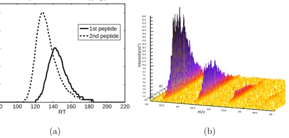
FIGURE Page 6 Overlapping signals of the first pair in 16-mix. a) Overlapping LC
profiles of the two peptides. (b) Signal peaks of the two peptides at charge state 1 in a 3D view. SNR at this region is quite low,
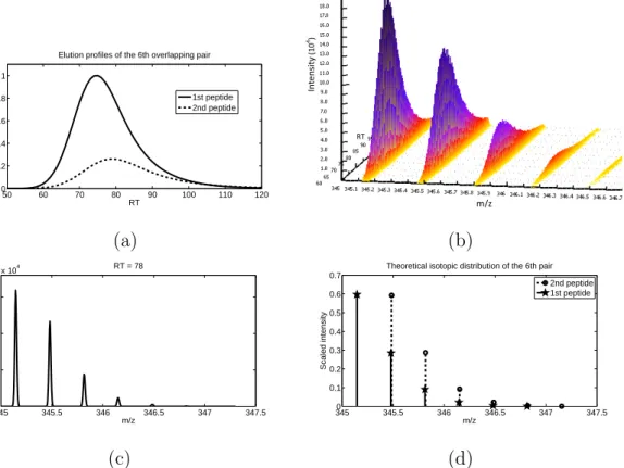
and significant peak overlapping can be observed. . . 53 7 Overlapping signals of the sixth pair in 16-mix. (a) Overlapping
LC profiles. (b) Signal peaks of the two peptides at charge state 3 in a 3D view. This region has a high SNR, where peaks of the 2nd peptide almost get completely shadowed by all but the first isotope peak of the 1st peptide. (c) MS scan sampled at 78s showing signals of the same pair. The observed overall signal pattern deviates from (d) the theoretic isotope patterns of the two
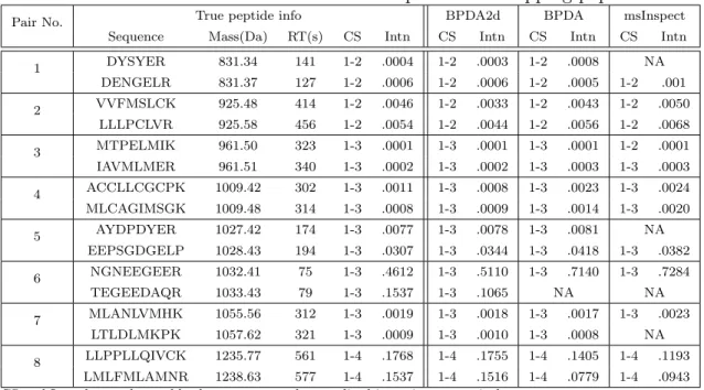
peptides. . . 54 8 Box plots of (a) absolute mass deviation and (b) normalized
inten-sity deviation of BPDA2d, BPDA and msInspect for the 16-mix
data set . . . 57 9 Detection results of the QTOF LC-MS/MS data set. BPDA2d,
BPDA and msInspect detected (a) number of features that can be matched to MS2 identifications at various significance levels and (b) total number of features. At significance level 0.05, the following two panels are obtained: (c) Histogram of normalized in-tensity of features detected by BPDA2d but not msInspect. Most of the features are from the low intensity region. (d) Box plots of
absolute mass deviation of different algorithms. . . 61 10 The proposed MS-based proteomics pipeline. . . 64 11 The MS calibration curve which displays the MS ion signal as a
function of analyte concentration in solution. The slope of the linear portion of the curve is the instrument response factor (i.e. instrument sensitivity). The curve departs from linear at high analyte concentration. A wider linear dynamic range is desired
FIGURE Page 12 Various quantities plotted as a function of the lower bound of
peptide efficiency factor (the upper bound is fixed at 1). (a) Mean quantification error as defined in Eq. 4.12. (b) Percent-age of observed differentially expressed marker proteins at a 0.05 significance level. (c) Missing value rates at the protein and pep-tide levels. (d) Classification error rates given by LDA and KNN
classifiers, respectively. . . 76 13 Effect of peptide efficiency factor on (a) differential expression
re-sults, and (b) classification errors for samples with reduced marker concentration. Results deteriorate compared to those using the
default protein concentration (Fig. 12(b) and 12(d)). . . 78 14 Effect of sample sizeM on (a) differential expression results, and
(b) classification error rates. All results generally improve as M increases. In (b) the classification error of the original protein sample (dashed lines) is plotted side by side with that of the ob-served protein data (solid lines), illustrating the substantial loss
in accuracy introduced by the MS analysis pipeline. . . 79 15 Effect of instrument response factorκ on (a) missing value rates,
(b) quantification accuracy, (c) differential expression results, and (d) classification error rates. As κ increases, all performance
in-dices improve quickly and then level off. . . 80 16 Effect of instrument response κ in the presence of saturation on
(a) missing value rates, (b) quantification accuracy, (c) differen-tial expression results, and (d) classification error rates. As κ increases, all performance indices at first improve and then de-teriorate (except for the peptide missing value rate, which levels
off). . . 81 17 Effect of noise on (a) missing value rates, (b) quantification
ac-curacy, (c) differential expression results, and (d) classification error rates. The x-axis represents α in the noise model given by Eqs. 4.7–4.8, while β is set to be 120α. The parameter values in the middle of the range (α= 0.04, β = 4.8) were estimated by an
FIGURE Page 18 Effect of using three hypothetic detection algorithms with
increas-ingly better performance, quantified by the (a) TPR vs. signal strength curves. The applications of the three algorithms lead to increasingly improved results in terms of ((b) missing value rates, (c) quantification accuracy, (d) percentage of detectable markers,
and (e) classification error rates. . . 85 19 Performance of a typical peptide detection algorithm in the second
category described in the text under various mass resolutions and in the presence of overlapping peptides. (a) Missing value rates, (b) quantification accuracy, (c) differential expression results, and
(d) classification errors. . . 86 20 Effect of MS2 replication on (a) missing value rates, (b)
quantifica-tion accuracy, (c) differential expression results, and (d) classifica-tion errors. It can be seen that replicate analysis can significantly boost peptide and protein identification rates, quantification and
classification results even only a few replicates are made available. . . 88 21 Simulation flow chart. . . 105 22 Effect of noise level. The classification error of the signal dataset
(signal), the measured dataset (orgn), and the five imputed datasets. The underlying distribution parameters are: SD σu = 0.4, gene correlation ρ = 0.7, MV rate r = 10%. Each panel in the figure corresponds to one combination of the feature selection methods and the classification rules, which is given by the title. The x-axis labels the number of selected genes, the y-axis is the noise level,
and the z-axis is the classification error. . . 110 23 Effect of variance. The classification error of the signal dataset
(signal), the measured dataset (orgn), and the five imputed datasets. The underlying distribution parameters are: noise levelµe= 0.2, gene correlationρ= 0.7, MV rater= 15%. Each panel in the fig-ure corresponds to one combination of the featfig-ure selection meth-ods and the classification rules, which is given by the title. The x-axis labels the number of selected genes, the y-axis is the signal
FIGURE Page 24 Effect of correlation. The classification error of the signal dataset
(signal), the measured dataset (orgn), and the five imputed datasets. The underlying distribution parameters are: SD σu = 0.5, noise level µe = 0.2, MV rate r = 10%. Each panel in the figure corre-sponds to one combination of the feature selection methods and the classification rules, which is given by the title. The x-axis labels the number of selected genes, the y-axis is the gene
corre-lation strength, and the z-axis is the classification error. . . 113 25 Effect of MV Rate. The classification error of the signal dataset
(signal), the measured dataset (orgn), and the five imputed datasets. The underlying distribution parameters are: SD σu = 0.3, gene correlation ρ = 0.7 and noise level µe = 0.2,0.2,0.3,0.3,0.4,0.4 for subfigures (a)-(f), respectively. The x-axis labels the number of selected genes, the y-axis is the MV rate, and the z-axis is the
classification error. . . 115 26 Effect of MV Rate. The classification error of the signal dataset
(signal), the measured dataset (orgn), and the five imputed datasets. The underlying distribution parameters are: SD σu = 0.4, gene correlation ρ = 0.7 and noise level µe = 0.2,0.2,0.3,0.3,0.4,0.4 for subfigures (a)-(f), respectively. The x-axis labels the number of selected genes, the y-axis is the MV rate, and the z-axis is the
classification error. . . 116 27 Effect of MV Rate. The classification error of the signal dataset
(signal), the measured dataset (orgn), and the five imputed datasets. The underlying distribution parameters are: SD σu = 0.5, gene correlation ρ = 0.7 and noise level µe = 0.2,0.2,0.3,0.3,0.4,0.4 for subfigures (a)-(f), respectively. The x-axis labels the number of selected genes, the y-axis is the MV rate, and the z-axis is the
classification error. . . 117 28 The NRMSE values (y-axis) of the five imputation algorithms
with respect to the MV rate (x-axis). The underlying distribution parameters are: SDσu = 0.5, noise levelµe = 0.2, gene correlation
FIGURE Page 29 The classification errors of the measured prostate cancer dataset
(orgn), and the five imputed datasets. Each panel in the figure corresponds to one combination of the feature selection methods and the classification rules, which is given by the title. The x-axis labels the number of selected genes, the y-axis is the MV rate,
and the z-axis is the classification error. . . 120 30 The classification errors of the measured breast cancer dataset
(orgn), and the five imputed datasets. The meanings of the axes
and titles are the same as in the previous figure.. . . 121 31 The NRMSE values (y-axis) of the five imputation algorithms
with respect to the MV rate (x-axis) for the PROST dataset and
CHAPTER I
INTRODUCTION
Translational science translates multidisciplinary scientific research into clinical prac-tice with the goal of aiding diagnosis, discovering new drugs, developing more effective treatments, and thus improving human health. Translational research may have dif-ferent meaning to difdif-ferent researchers, but it seems important to almost everyone [1]. There are generally two paths in the practice of translational research. One is data-driven and the other is goal-driven. The former tries to make sense of the data, link the observed phenomenon with scientific explanations, or apply pattern recognition to discover features that can be associated to phenotypes. The latter follows the guidance of a goal, which usually leads to carefully designed experiments and conceptualization of the translational problem [2]. In this dissertation, we adopt the goal-driven approach, which is more of a systems engineering approach.
For “conceptualization”, a model-based approach is undoubtedly a beneficial way to go as proved by the successful development and application of many well known methods such as ANOVA for microarray data analysis [3], hypothesis testing for biomarker detection, and controlling false positive identifications via decoy databases in mass spectrometry (MS) based proteomics [4, 5]. The beauty of model-based ap-proach lies in that by mathematical formalization of the problem, key issues and factors can be captured, optimal solutions can be achieved, and the gained insights can be translated into prediction or control of the underlying system. It should be noted that the conceptualization should be formed at the right level of abstraction: The model must be sufficiently complex to represent the characteristics or behaviors
of the physical system, while at the same time it must be simple enough that the necessary parameters can be well estimated and the optimization problem is compu-tationally tractable [2].
In translational science, most research is carried out on the molecular level which study the fundamental building blocks of living organisms—DNA, RNA and protein as well as their interactions. The terms “genomics” and “proteomics” were coined for the two major branches concerning the study of genomes and proteins of organisms, respectively. Ever since the the advent of DNA microarrays in the mid-1990s, the development of related analytical equipments and methods has boomed. Microarray and next generation sequencing for genome-wide gene profiling, mass spectrometry for large scale protein analysis, along with other high-throughput technologies greatly expand the experimental capabilities and propel the research.
In this chapter, the high-throughput technologies related to the research con-ducted for the dissertation are briefly reviewed. The challenges in genomic and pro-teomic data analysis and the problems with existing methods are outlined, which bring forward the proposed methodology for biomarker detection and systematic analysis.
A. MS-based proteomics
Mass spectrometry is a key analytical tool in proteomics. It is widely used for large-scale protein profiling with applications in biomarker discovery [6], signaling pathway monitoring [7, 8], drug development, and disease classification [9]. A mass spectrom-eter measures the concentration of ionized molecules at a range of mass-to-charge ratios (m/z). MS instruments consist of three modules: an ionization source, a mass analyzer and a detector which captures the ions and measures the intensity of each ion species. Widely used ionization methods include electrospray ionization (ESI) [10] and
matrix-assisted laser desorption/ionization (MALDI) [11, 12]. Mass analyzers sepa-rate the ions according to their mass-to-charge ratios. There are several types of mass analyzers including the Orbitrap [13], Quadrupole [14], Time-of-Flight (TOF) [15,16], and Fourier transform ion cyclotron resonance (FTICR) [17].
In a typical MS experiment, unknown protein mixtures extracted from biological samples are first digested into peptides by enzymes such as trypsin. Then peptides enter a mass spectrometer where they get ionized and separated according to their mass-to-charge ratios. As a result, a spectrum is produced which plots the ion inten-sity against the mass-to-charge ratio. The recorded intensities reflect the abundance or concentration of peptides. Liquid Chromatography (LC) is often coupled with MS to achieve additional separation of peptides and thus reduce the complexity of an individual mass spectrum: before entering the mass spectrometer, peptides are first passed through an LC column where they are separated by the retention time, depending on their physicochemical properties and interactions with the solvent. A single LC-MS experiment usually produces hundreds to thousands of mass spectra sampled during the LC elution process.
Analysis of LC-MS experiments by computational methods is challenging due to the huge data size and rich information content, and moreover is complicated by several facts including: (1) Proteins contained in complex samples such as plasma and tissue extracts have a wide dynamic concentration range (e.g. 10 orders of mag-nitude), plus peptides differ in ionization efficiencies, which means that the observed peptide signal from MS data may also have a wide dynamic range. While high abun-dance peptides are relatively easy to be identified, low abunabun-dance peptides/proteins, which are often of more biological importance, are likely to be buried under noise or interfering signals and thus hard to be detected [18]. (2) The shape of peptide chromatographic peaks is not well predicted [19]. Due to experiment settings and the
nature of the analytes, asymmetric shape or plateaus of chromatographic peaks may be observed, which requires designed detection algorithms to be robust in tracking signals from various peptide species and be adaptable across experiments. (3) A pep-tide species may register several groups of peaks in different regions of the spectra due to the following two points: first, a peptide species may take various numbers of charges during ionization, therefore its peaks can be observed at different charge states; second, at a given charge state, several peaks with equal spacing can be ob-served due to heavy isotopes (e.g. 13C), which are commonly referred to as isotopic
peaks or the isotope series. Correctly identifying all the peaks and assigning them to the right peptide is a non-trivial task. (4) The signal density can be very high even in high-resolution LC-MS data and overlapping peptide peaks are commonly observed, the detection of which is very challenging.
1. Feature extraction in MS data analysis
Peptide detection and identification, which extracts features from the raw spectra and converts the raw data into a list of peptides, is usually the first step in MS data processing. It is a critical step that directly affects the accuracy of subsequent analysis, such as protein identification and quantification, data alignment between multiple experiments, biomarker discovery, and sample classification.
Fragmentation spectra produced by tandem mass spectrometry (MS2) are fre-quently used by popular software such as SEQUEST and Mascot [20] for database searching to give peptide identifications. However, only a small percentage of peptides present in the sample get selected for fragmentation analysis, and of these selected peptides even fewer can be correctly identified by database searching due to spectrum matching ambiguity or co-eluting precursor ions [21]. Furthermore, quantitation of peptide abundance based on MS2 spectral counting is quite rough, and highly
vari-able especially for low abundance peptides [22]. (Though by using well established stable isotope labeling approaches such as tandem mass tags, the relative abundance of analytes in different samples can be accurately determined [23].)
Therefore many algorithms for peptide detection are designed to use MS1 infor-mation directly, and thus have the potential to identify more peptides. When mass spectra have low resolution in which isotopic peaks cannot be baseline resolved (i.e. the isotopic peaks convolve together to form isotope envelopes, and only one peak can be observed for one peptide at a given charge state), and when peptides are singly charged as commonly observed in MALDI, to report each detected peak as a peptide feature might be sufficient, as done in [24–27]. But for high resolution spectra, report-ing each observed peak as a unique peptide species would give rise to too many false positives. Thus a variety of algorithms for deisotoping and charge states deconvolution have been proposed. Such algorithms can be mainly divided into two categories: one-dimensional (1D) algorithms (e.g. NITPICK [28], PepList [29], Decon2LS [30] and Hardkl¨or [31]), which perform peak picking, deisotoping and charge state assignment on a scan-to-scan basis, and two-dimensional (2D) algorithms (e.g. MZmine [32], SpecArray [18], msInspect [33], SuperHirn [34], VIPER [35], MaxQuant [36], and OpenMS [37]), which capture the 2D nature of LC-MS data and utilize informa-tion from both the mass-to-charge and reteninforma-tion-time (RT) dimensions for peptide detection. 2D algorithms appear to be more promising in handling LC-MS data. Regardless of category, most of the aforementioned algorithms are grounded on the idea of greedy template-matching which makes them ineffective to detect overlapping and low abundance peptides. This motivates the development of a global optimiza-tion based Bayesian peptide detecoptimiza-tion algorithm for feature extracoptimiza-tion and peptide detection.
2. MS analysis pipeline for biomarker discovery
In clinical applications of mass spectrometry, the number of samples available is usually in the range of tens to a few hundred (small sample size). The samples are analyzed by an MS instrument and transformed into a series of mass spectra containing hundreds of thousands of intensity measurements with signal generated by thousands of proteins/peptides (large feature dimension). This small-sample, high-dimensionality problem requires the experiment and analysis to be carefully designed and validated in order to arrive at statistically meaningful results.
The MS analysis pipeline consists of many steps, including sample preparation, instrument analysis, feature extraction, quantification, statistic analysis and so on. The pipeline can be viewed as a noisy channel, where each processing step introduces some loss or distortion to the underlying signal and the biomarker discovery results are affected by the combined effects of all upstream steps. While individual components of the MS pipeline have been studied at length, little work has been done to integrate the various modules, evaluate them in a systematic way, and focus on the impact of the various steps on the end results of differential analysis and sample classifica-tion. In real experiments, it is not easy to decouple the compound parameter effects and determine the marginal influence of various modules on the end results, due to variations and the complicated nature of the workflow. Moreover, owing to contam-inants and unknown or incomplete ground-truth, it is hard to meaningfully evaluate and compare results across different experiments. Thus we propose a model-based approach to evaluate the pipeline systematically. It allows us to better understand the characteristics of the MS data, the contributions of individual modules, and the performance of the full pipeline.
B. DNA microarray-based genomics
DNA microarrays are small, solid supports onto which the sequences from large num-bers of genes are immobilized at fixed locations, known as probes. Based on probe-target hybridization, the microarrays can be used to measure the expression levels of hundreds and thousands of genes simultaneously. It revolutionizes the way scien-tists examine gene expression, but also poses many challenges in the analysis of the resulting high-dimension small-sample data sets.
Microarray data frequently contain missing values (MVs) because imperfections in data preparation steps (e.g. poor hybridization, chip contamination by dust and scratches) create erroneous and low-quality values, which are usually discarded and referred to as missing. It is common for gene expression data to contain at least 5% MVs and, in many public accessible data sets, more than 60% of the genes have MVs [38].
There exists many imputation methods for estimating MVs. But only a few studies have examined the impact of MV imputation on high level analysis such as sample clustering and classification. Furthermore, these studies are problematic in key steps such as MV generation and classifier error estimation. To address these problems, a model-based approach is developed to explore the relationship among the data quality, MVs and high level analysis in the microarray data analysis pipeline.
C. Organization of the dissertation
This thesis is organized as described below.
Chapter II proposes a Bayesian approach, BPDA, for peptide detection in MS data, such as MALDI-TOF and LC-MS, with high enough resolution [39]. BPDA is based on a rigorous statistical framework and avoids problems, such as voting and
ad-hoc thresholding, generally encountered in algorithms based on greedy template-matching. It systematically evaluates all possible combinations of possible peptide candidates to interpret a given spectrum, and iteratively finds the best fitting peptide signal in order to minimize the mean squared error of the inferred spectrum to the observed spectrum. In contrast to previous methods, BPDA performs deisotoping and deconvolution of mass spectra simultaneously, which enables better identification of weak peptide signals and produces higher sensitivity results. Unlike template-matching algorithms, BPDA can effectively handle overlapping peptide features. Ex-perimental results indicate that BPDA performs well on both simulated data and real data, for various resolutions and signal to noise ratios, and compares very favorably with commonly used commercial and open-source software.
Chapter III proposes a 2D Bayesian peptide detection algorithm, BPDA2d, which extends the previous work [40]. BPDA2d is specially designed for LC-MS. It models the spectra from both m/z and RT dimensions, thereby better capturing and fitting the properties of LC-MS data. Instead of local template matching, BPDA2d performs global optimization for all possible peptide candidates and systematically optimizes their signals. Since BPDA2d looks for the optimal among all possible interpretations of the given spectra, it has the capability in handling complex spectra where fea-tures overlap. For each peptide candidate, BPDA2d takes into account its elution profile, charge state distribution, and isotope pattern, and it combines all evidence to infer the signal and existence probability of the candidate. By piecing all evidence together — especially by deriving information across charge states — low abundance peptides can be better identified and peptide detection rates can be improved. Our experiments indicate that BPDA2d outperforms state-of-the-art detection methods on both simulated data and real LC-MS data, according to sensitivity and detection accuracy.
While Chapter II and III focus on enhancing the feature extraction module in the MS analysis pipeline, Chapter IV investigates the entire pipeline from a systems point of view. A model-based approach is presented to integrate various pipeline modules and evaluate the pipeline systematically, by means of simulation with ground-truthed data [41]. Key steps and factors of the pipeline are captured, and their effects on peptide identification rate, protein quantification accuracy, differential expression results, and classification accuracy are studied. The proposed MS-based proteomics framework can be used to optimize the workflow and predict experiment results.
Chapter V extends the system approach presented in Chapter IV to the analysis of DNA microarray data. In this chapter, a model-based approach is developed to examine the effects of MVs and their imputation on classification in a complicated microarray data analysis pipeline [42]. Six popular imputation algorithms, two feature selection methods, and three classification rules are considered. The situations when it is suitable to apply MV imputation are identified and recommendations regarding imputation are provided.
Chapter VI summarizes the dissertation and proposes future research directions.
D. Main contributions
The main contributions of this work are summarized below:
• Developed Bayesian peptide detection algorithms to optimize the feature ex-traction step in MS-based proteomics. The algorithms can effectively identify low abundance peptides and overlapping peptides, which is not satisfactorily addressed by existing approaches. The proposed methods achieved better sen-sitivity and accuracy results compared to many popular software packages.
sys-tematic evaluation of the MS data analysis pipeline. By contrast, in previous methods the pipeline is frequently chopped up into individual modules, and is rarely studied and assessed as a whole from a systems point of view. The proposed framework can be used to determine the working range of important parameters, aid experimental design, predict the biomarker discovery results, and to pinpoint critical bottlenecks which are worth investing resources into for improving performance.
• Proposed a model-based approach to examine how different properties of a microarray data set influence the quality of the imputed data and how missing value imputation influence the classification performance. The results suggest that it is beneficial to apply MV imputation when the noise level is high, variance is small, or gene-cluster correlation is strong, under small to moderate MV rates. In addition, an MV-rate related peaking phenomenon was uncovered.
CHAPTER II
BAYESIAN PEPTIDE DETECTION FOR MASS SPECTROMETRY∗ A. Background
Feature extraction, which includes peptide detection and quantification, is usually the first step in MS data processing pipeline. Accurate detection and quantification of peptides and proteins is essential for biomarker discovery, drug development and disease classification.
A variety of algorithms for peptide detection in high resolution mass spectra have been proposed. Most of these algorithms are grounded on the idea of greedy template-matching. Such algorithms include PepList [29], Decon2LS [30], Noy’s method [43], MZmine [32], SpecArray [18], msInspect [33], SuperHirn [34], VIPER [35], and OpenMS [37]. The templates used are often based on theoretic isotope pat-terns calculated from peptide masses [44]. If an observed group of peaks matches the proposed template well — the quality of the match is usually assessed by a fitting score — it will be reported as a feature and then subtracted from the spectra. The matching and subtraction process goes on until no more matches can be found. The major problem with greedy template-matching is that it may be ineffective to detect overlapping peptides. In the case of overlapping (e.g. one doubly charged peptide can overlap with a singly charged peptide of half the mass given that the two elute from chromatography column at a similar time), if the peak group of one peptide is incorrectly matched and subtracted, the rest of the overlapping peptides cannot be
∗Reprinted with permission from “BPDA—a Bayesian peptide detection
algo-rithm for mass spectrometry” by Y. Sun, J. Zhang, U. M. Braga-Neto, and E. R. Dougherty, BMC Bioinformatics, vol.11, pp. 490-500, 2010, Copyright 2010 by BioMed Central.
detected correctly using the remaining signal, which may result in error propagation. Besides, each template is aimed at matching isotopic peaks of one single peptide, and thus are likely to be different from the observed overlapping peaks, which ren-ders a poor match and reduces the sensitivities of these algorithms. Alternatives to greedy template-matching based approaches include 1D algorithms such as NITPICK, which is based on non-greedy regression; Hardkl¨or, which approximates an isotope peak cluster by a set of averagine models [45]. They also include 2D algorithms such as MaxQuant, which mainly relies on the distance among isotope peaks and the cor-relation between isotope labeled (SILAC) pairs to detect and quantify peptides in SILAC-proteome experiments.
In this chapter, we propose a Bayesian Peptide Detection Algorithm (BPDA) to optimize the workflow of peptide deisotoping and charge state deconvolution. BPDA can be applied to data generated by MS instruments with mass resolutions high enough to baseline-resolve isotopic peaks. It evaluates all possible combinations of possible peptide candidates (originated from well-defined peaks of the raw spectrum — see Methods section for more details) to interpret a given spectrum, and iteratively finds the best fitting peptide parameters (peptide peak heights, existence probabili-ties, etc.) in order to minimize the mean squared error (MSE) of the inferred spectrum to the observed spectrum.
B. Methods
For 1D MS spectrum, we first perform spectrum preprocessing to remove the baseline, filter the noise and generate a list of peptide candidates. Then BPDA is applied based on the developed MS model to infer the best fitting peptide signals of the observed spectrum, the results being peptide abundances, existence probabilities and so on.
For 2D LC-MS spectra, we first detect peptide elution peaks along the retention time dimension, and build elution peak groups by collecting the peaks which have similar retention time together using a method similar to [46]. Each group contains a series of consecutive spectra, which are then averaged to form a mean spectrum. The rationale of using a mean spectrum to represent the group is that the noise of consecutive spectra could be canceled out to a certain degree [24]. The BPDA algorithm is then applied to each of the mean spectra, and finally an overall peptide list is generated. The details of the preprocessing step, the proposed MS model, and the BPDA algorithm are described in the following subsections.
1. Spectrum preprocessing and obtaining peptide candidates
A non-flat baseline is often observed in mass spectra, the presence of which can distort the true signal pattern. Thus the first preprocessing step is to detect and subtract the baseline from MS spectra. We use the minimum of a sliding window along them/z axis as the baseline, similar to the method used in [47]. The next step is peak detec-tion. We use the Matlab function “mspeaks” (http://www.mathworks.com/access/ helpdesk/help/toolbox/bioinfo/ref/mspeaks.html) to perform this task. The algorithm first identifies all local maxima in the wavelet denoised spectrum as puta-tive peak locations. Then peaks are filtered based on their intensities and signal to noise ratios. The last step of preprocessing is to obtain a list of peptide candidates. Considering one detected peak with centroid at m/z value d, we want to find out which peptides can potentially register a peak at this position. The answer is given below in terms of the masses of such peptides:
where mass is the mass of one peptide candidate, mpc is the mass of one positive charge and mnt is the mass shift caused by addition of one neutron. Due to mass defect, the mass shift varies for different elements. We approximate mnt using the mass shift from 13C to 12C, which is 1.0034, since Carbon contributes most to the
isotope patterns. This approximation works well if the mass calibration of the instru-ment is correct. The parameters cs and iso are user defined maximum numbers of considered charge states and isotopic positions, respectively. It is easy to see from the above equation that each detected peak gives rise to cs×(iso+ 1) different peptide candidates (masses). These candidates exhaust all the possibilities to generate the peak with centroid d, but it does not follow that all the candidates really exist in the sample. Therefore, our primary goal in peptide detection is to find the existence probability of each peptide candidate. Also note that the total number of candidates should be less than or equal tocs×(iso+1)×number of detected peaks, as is possible that multiple peaks yield the same candidate mass.
2. Modeling the mass spectrum
Suppose N peptide candidates are obtained from the observed spectrum using the method described in the previous section. Each candidate can generate a series of peaks over different charge states, and at each charge state several isotopic peaks can be registered. The signal generated by thekth peptide candidate is thus modeled by the following equation, in which i and j represent the charge state and the isotopic position of the candidate peptide, respectively:
gk(xm) = cs X i=1 iso X j=0
ck,ijf(xm;ρk,ij, αk,ij), m= 1,2, . . . , M, (2.2) where the peak shape function is given by f(xm;ρk,ij, αk,ij) = e−ρk,ij(xm−αk,ij)
2
That is, the peak is modeled as Gaussian-shaped, as in [19]. It is reported that the Gaussian-shaped peak approximates the reality well enough to obtain good detection results [43]. Still, this peak shape function can be adjusted for different instruments without affecting the overall structure of the algorithm.
The observed spectrum is a mixture of the signal generated by the N peptide candidates plus Gaussian random noise, which can be modeled as:
ym = N X k=1 λkgk(xm) +m = N X k=1 λk cs X i=1 iso X j=0
ck,ijf(xm;ρk,ij, αk,ij) +m, (2.3) m= 1,2, . . . , M.
In the above three equations, xm is the mth mass-to-charge ratio (m/z) in the spectrum,ym is the observed intensity at xm, M is the number of observations, and m is Gaussian random noise with zero mean and standard deviation σ. The value ofσ can be approximated by the standard deviation of the background region in the spectrum. Note that we model m as additive Gaussian which is generally a good model for the thermal noise in electronic instruments. There are reports of non-Gaussian noise in FTMS [48] and thus it is safer to apply the proposed algorithm to TOF MS instruments [49]. The parameters of the kth candidate, namely, αk,ij,ρk,ij, λk and ck,ij are discussed in detail below:
• αk,ij is the theoretic centroid (m/z value) of the peak generated by candidate k, at charge state i and isotopic number j.
αk,ij =
massk+i mpc+j mnt
i , i= 1,2, . . . , cs, j = 0,1, . . . , iso, (2.4) where massk is the mass of the kth candidate. Since the candidate’s mass is already obtained, αk,ij can be calculated.
• ρk,ij relates to the shape (width) of the peak centered at αk,ij. It can be es-timated by using its relationship to the peak’s Full Width at Half Maximum (FWHM): ρk,ij = 2√2 ln 2/FWHM.
• λkis an indicator random variable, which is 1 if the kth peptide candidate truly exists in the sample and 0 otherwise.
• ck,ij is the height (i.e. intensity) of the peak generated by peptide k, at charge state i and isotopic number j.
In summary, the model considers peaks at different isotopic positions and charge states simultaneously for each peptide candidate, incorporating candidates’ existence probabilities and the spectrum thermal noise.
3. Bayesian peptide detection Let
θ,{λk, ck,ij;k = 1, . . . , N, i= 1, . . . , cs, j = 0, . . . , iso}
be the set of all the unknown model parameters. The goal of our algorithm is to determine the value ofθ based on the observed spectrum y= [y1, . . . , yM]T. In fact,
the value of λk is of our prime interest for the peptide detection problem. For this purpose, we can use a Bayesian approach to first obtain the a posteriori probability (APP) of all the parameters,P(θ|y). Then the APPs P(λk|y), k= 1, . . . , N, can be obtained by integration of the joint posterior distributionP(θ|y) over all parameters exceptλk. Clearly, the calculation involves high dimension integration which is not an easy task. Besides, due to the highly nonlinear nature of the data model, none of the desired APPs can be obtained analytically. To overcome the computational obstacle, we resort to the Gibbs sampling method [50], which is a variant of the Markov Chain
Monte Carlo (MCMC) approach [51], to sample the model parameters.
Gibbs sampling is an iterative scheme, which uses the popular strategy of divide-and-conquer to sample a subset of parameters at a time while fixing the rest at the sample values from the previous iteration, as if they were true. In other words, for the lth parameter group θl, we sample from the conditional posterior distribution P(θl|θ−l,y), where θ−l , θ \θl. After this sampling process iterates among the parameter groups for a sufficient number of cycles (which is referred to as the “burn-in” period), convergence is reached. The samples collected afterwards are shown to be from the marginal posterior distributionP(θl|y), which is independent ofθ−l, and thus these samples can be used to estimate the target parameters.
The Gibbs sampling process for the kth peptide candidate and the derivations of the conditional posterior distributions of important model parameters are detailed below.
a. Sampling the peak height vector
The heights of all the possible peaks (over different charge states and isotopic posi-tions) of thekth peptide candidate are included in the peak height vector ck, which is defined as ck , [ck,ij;i = 1, . . . , cs, j = 0, . . . , iso]T. By the Bayesian principle, the conditional posterior distribution ofck is proportional to the likelihood times the prior:
P(ck|y,θ−ck)∝P(y|θ)Prior(ck), (2.5) whereθ−ck ,θ\ck.
It is easy to show the likelihood satisfies P(y|θ)∝exp{− 1
2σ2(y−Gλ (0)−λ
where λ(s),[λ1, . . . , λk =s, . . . , λN]T, s∈ {0,1}, (2.7) G= g1(x1) g2(x1) . . . gN(x1) g1(x2) g2(x2) . . . gN(x2) .. . ... . .. ... g1(xM) g2(xM) . . . gN(xM) M×N , (2.8)
with the (m, k)-th entry gk(xm) = cs P i=1 iso P j=0
ck,ijf(xm;ρk,ij, αk,ij) representing the signal atm/z valuexm generated by peptide candidate k. In addition,
Hk = [hm,(i−1)×(iso+1)+j+1]M×cs(iso+1), withhm,(i−1)×(iso+1)+j+1 =
f(xm;ρk,ij, αk,ij) =e−ρk,ij(xm−αk,ij)
2
.
The heights of the isotopic peaks of peptide candidate k at charge state i fol-low a multinomial distribution [52], which by the Central Limit Theorem can be approximated by a Gaussian distribution as below:
P(ck,ij, j = 0, . . . , iso|ak, ηk,i,πk) = M N(akηk,i,πk) (2.9)
≈ N(akηk,iπk,
akηk,i[diag(πk)−πkTπk]), (2.10) whereak is the total centroid intensity of candidatek, and ηk ,[ηk,1, ηk,2, . . . , ηk,cs]T
and πk,[πk,0, πk,1, . . . , πk,iso]T denote the charge state distribution and the theoret-ical isotopic distribution of peptide candidate k, respectively.
Thus the prior distribution of the peak height vectorck is given by:
where µck = [akηk,1π T k, akηk,2πkT, . . . , akηk,csπ T k] T , (2.12) Σck = diag(Σi), (2.13) with Σi = akηk,i[diag(πk)−πkTπk], i= 1,2, . . . , cs. (2.14) Substituting Eq. 2.6 and Eq. 2.11 into Eq. 2.5 and it can be shown by algebraic manipulations [53] that the conditional posterior distribution of ck is also Gaussian, with the mean vector and covariance matrix given below:
Σc k|y,θ−ck = (I−KHk)Σck, (2.15) µc k|y,θ−ck = µck +K(y−Gλ (0)−H kµck), (2.16) where K , ΣckH T k HkΣckH T k +σ2IM×M −1
is known as the Kalman gain matrix [54].
b. Sampling the total centroid intensity
The total centroid intensity of candidate k is denoted by ak, whose conditional dis-tribution takes different forms for different values of λk.
When λk = 1 (the kth candidate is inferred to be present), by definition, ak|(ck,ij, λk= 1) = cs X i=1 iso X j=0 ck,ij ·Ick,ij>0. (2.17) Whenλk= 0 (the kth candidate is inferred to be absent), the distribution of ak, which is independent of the observation ck, is modeled by a uniform distribution as
below:
P(ak|ck,ij, λk= 0 ) = Unif(0, uk), (2.18) whereuk is the upper bound of ak.
c. Sampling the charge state distribution
Let ηk , [ηk,1, ηk,2, . . . , ηk,cs]T denote the charge state distribution of peptide can-didate k. Unlike the isotopic distribution, the charge state distribution cannot be theoretically predicted even when the peptide sequence is given. Thus ηk needs to be estimated by the Gibbs sampling process. Let bk , [bk,1, bk,2, . . . , bk,cs]T, where bk,i is the total centroid abundance of peptide k at charge state i. Given the charge state distribution and the total centroid abundance of peptidek, the likelihood of bk is multinomial:
P(bk|ηk, ak) = MN(ak,ηk). (2.19) As is well known, the conjugate prior to a multinomial likelihood is Dirichlet, which is also a reasonable choice for the prior of ηk. Thus, let the prior of ηk be a Dirichlet distribution with parameter wα, where w is a weight parameter that controls the strength of the prior information. A small w is preferable if uncertainty resides in the prior, and vice versa. Then the posterior distribution ofηk is given by P(ηk|bk) ∝ P(bk|ηk)Prior(ηk) (2.20) = Dirichlet(wα+bk). (2.21)
d. Sampling the peptide existence indicator variable
The conditional posterior distribution ofλk, the existence indicator variable of peptide k, is given by P(λk|y,θ−λk) ∝ P(y|θ)Prior(λk) ∝ exp{− 1 2σ2ky−Gλk 2}Prior(λ k), (2.22)
where G is defined in Eq. 2.8.
The log-likelihood ratio (LLR) ofλk can be calculated as below LLRλk = ln P(λk = 1|y,θ−λk) P(λk = 0|y,θ−λk) = − 1 2σ2(ky−Gλ (1)k2− ky−Gλ(0)k2) + lnP(λk = 1) P(λk = 0) , (2.23) whereλ(s), s∈ {0,1} is defined by Eq. 2.7.
If no prior knowledge is available about which peptide candidates are more likely to be present in the sample, then a reasonable choice for the prior of λk could be the uniform distribution. Therefore the last term in Eq. 2.23 can be dropped. The conditional posterior distribution of λk is then obtained based on the log-likelihood ratio as follows:
P(λk= 1|y,θ−λk) =
1
1 +e−LLRλk, (2.24)
P(λk= 0|y,θ−λk) = 1−P(λk = 1|y,θ−λk). (2.25) The complexity of the proposed Gibbs sampling algorithm is determined by two factors: (1) the sheer number of peptide candidates, and (2) the correlation between parameters that need to be sampled. The algorithm complexity grows exponentially with the number of peptide candidates, and the correlation between parameters re-duces the sampling efficiency. To address these two issues, we first partition
non-overlapping peptide candidates into different groups. The proposed algorithm can be applied to each group in a parallel manner and the algorithm complexity is reduced, because within each group the number of candidates is reduced, and the corresponding signal-containing spectrum region is restricted. Peptide candidates within each group are then clustered by the k-means clustering algorithm [55], the distance measure be-ing the correlation between peptide candidate signals. Peptide candidates within a cluster have strong correlations among each other, and their indicator variables are sampled from the joint conditional posterior distribution. These two measures improve the overall efficiency of the algorithm.
Samples taken after convergence can be used to estimate the target parameters. Particularly, the existence probability of peptidek is calculated as
P(λk= 1|y) = 1 R−r0+ 1 R X r=r0 λrk, (2.26)
where r0 is the first iteration after convergence is reached, R is the total number of
iterations, and λrk is the sample value of λk in the rth iteration. The kth peptide candidate is said to be detected if its existence probability P(λk = 1|y) is greater than a predefined threshold.
C. Results
We report below the observed performance of BPDA, side by side with well-known tools, such as OpenMS and Decon2LS, in a number of experiments using both syn-thetic and real data.
1. Synthetic data
It is difficult to evaluate the performance of a given detection method using real data due to the existence of unpredictable contaminants and the unknown true composition of the samples. The merit of using simulated data is that the ground truth is known and thus algorithm evaluation can be carried out [19, 49].
a. Synthetic 20-mix spectra with different abundance levels (SNRs)
First, to test the robustness of our algorithm, we generated MS data sets with different signal to noise ratios (SNRs), using the method described in [19]. In fact, the mean signal strength (i.e., peptide abundance) was varied while the noise level (i.e., the mean and variance of the noise) was fixed. For each peptide abundance level a, a ∈ {500,2500,12500}, the simulation was repeated 50 times. In each repetition, 20 true peptides (with abundance levelaand masses randomly selected from a quality-control Shewanella Oneidensis data set provided by PNNL (http://omics.pnl.gov) served as the input of the data model given by Eq. 2.3. The charge state distribution of one peptide was modeled by a binomial distribution, which was reported to approximate the real data well [19]. The isotopic distribution was obtained for each peptide by using the Averagine model [56] and the Mercury algorithm [44]. The output consists of a simulated mass spectrum. BPDA was applied to obtain the peptide existence probabilities and abundance results. Its performance was evaluated by the classic Receiver Operating Characteristic (ROC) curve. To obtain the ROC curve, first a series of detection levels τ ranging from 0 to 1 with 0.001 increments was selected. Peptides with existence probabilities not less thanτ were said to be detected at this specific detection level. The True Positive Rate (TPR) and False Positive Rate (TPR) were then calculated at each detection level as follows: T P R= T rueP ositiveT rueP ositive+F alseN egative
andF P R = F alseP ositiveF alseP ositive+T rueN egative. One ROC curve (each point on the curve was a pair of TPR and FPR at one detection level) was plotted for each repetition. And the averaged ROC curve for one abundance level was obtained by averaging all the ROC curves corresponding to the same abundance level. We also applied OpenMS on the same data sets — to do so, we first wrote the simulated MS data into a text file with three columns specified by elution time, m/z, and intensity, respectively. Next, the text file was converted to mzXML (which is a valid input file format for OpenMS) by the FileConverter tool integrated in the OpenMS software package (http://open-ms. sourceforge.net). Finally, OpenMS was applied on the mzXML file to give the detection results including detected features and their qualities. The ROC results given by the two algorithms for different abundance levels are shown in Fig. 1.
0 0.1 0.2 0.3 0.4 0.5 0.6 0.7 0.8 0.9 1 0 0.1 0.2 0.3 0.4 0.5 0.6 0.7 0.8 0.9 1 ROC curves FPR TPR BPDA−12500 BPDA−2500 BPDA−500 OpenMS−12500 OpenMS−2500 OpenMS−500
Fig. 1. ROC results for synthetic 20-mix spectra with different abundance levels a= 500,2500 and 12500.
b. Synthetic 10-mix spectrum with overlapping peptides
As noted before, overlapping peptide peaks can complicate the mass spectra and make the detection problem much harder. Thus, we investigated the performance of BPDA in the presence of overlapping peptides. A simulated 10-mix spectrum was generated by 5 pairs of overlapping peptides with unique masses: 1264.279, 1266.383, 1382.247, 1388.367, 1293.323, 1294.345, 1312.441, 1313.451, 1327.386 and 1329.378 Da. The detection results for the comparison between BPDA and OpenMS are summarized in Table I. BPDA detected all 10 peptides when F P R = 0.1, with very small mass deviations and quite accurate abundance results. Almost all charge states of the 10 true peptides were correctly reported, except for the highest charge state of the 5th and the 9th peptides. These two charge states were missed because the corresponding peptide signal was very weak. In contrast, whenF P R= 0.1, OpenMS only detected the 3rd, the 7th and the 9th peptides. And when FPR increased to 0.3, OpenMS achieved its highest TPR (0.6). But it could detect only one pair of peptides (the one with the least overlap) and missed one peptide in each of the other 4 pairs. Two examples are given in Fig. 2 to illustrate the observed overlapping peptide signals and the detection results. The abundance results given by OpenMS were not close to those of the true peptides (although the total abundance of each overlapping pair was not far away from the corresponding total abundance of the true peptides). In total, 18 out of 36 charge states were correctly detected by OpenMS for the 10 peptides, while BPDA correctly detected 34 out of 36, a much larger number.
We remark that Decon2LS results are missing from both synthetic experiments described previously because the synthetic data could not be loaded, causing the program to crash (the data was contained in a mzXML file converted from a 3-column text file by the OpenMS FileConverter tool, whose format was successfully
Table I. Results for the synthetic 10-mix data set with overlapping peptides. Intn, CS and dM denote the normalized intensity, detectable charge states and the mass deviation from the true mass, respectively. When FPR = 0.1, BPDA was able to detect all 10 true peptides, while OpenMS detected only 3 peptides (marked by *). OpenMS achieved its highest TPR (0.6) when FPR = 0.3.
BPDA OpenMS
True Mass (Da) / Intn / CS dM (Da) / Intn / CS dM (Da) / Intn / CS 1264.279 / 0.034 / 1-3 -0.0065 / 0.032 / 1-3 NA 1266.383 / 0.103 / 1-3 -0.0025 / 0.110 / 1-3 −0.0025 / 0.156 / 1-3 1382.247 / 0.171 / 1-4 0.0028 / 0.181 / 1-4 0.0031∗ / 0.228 / 1-3 1388.367 / 0.114 / 1-4 -0.0073 / 0.097 / 1-4 −0.0046 / 0.150 / 1-3 1293.323 / 0.006 / 1-3 -0.0081 / 0.007 / 1-2 NA 1294.345 / 0.008 / 1-3 -0.0124 / 0.008 / 1-3 0.0033 / 0.018 / 1-2 1312.441 / 0.229 / 1-4 0.0018 / 0.247 / 1-4 0.0019∗ / 0.334 / 1-4 1313.451 / 0.183 / 1-4 -0.0061 / 0.173 / 1-4 NA 1327.386 / 0.080 / 1-4 -0.0035 / 0.067 / 1-3 0.0061∗ / 0.114 / 1-3 1329.378 / 0.072 / 1-4 -0.0035 / 0.078 / 1-4 NA
27 647 647.5 648 648.5 649 649.5 650 650.5 0 100 200 300 400 m/z In te n s it 422 422.5 423 423.5 424 424.5 0 100 200 300 400 500 600 m/z In te n s it y Monoisotopic peak (a) 647 647.5 648 648.5 649 649.5 650 650.5 0 100 200 300 400 500 600 700 800 m/z In te n s it y Monoisotopic peak 422 422.5 423 423.5 424 424.5 0 100 200 300 400 500 600 m/z In te n s it y Monoisotopic peak (b)
Fig. 2. Illustration of overlapping peptides observed in the synthetic 10-mix spectrum. (a) Overlapping peptide signals observed inm/z range 422-424.5, which is gen-erated by monoisotopic masses 1264.28 and 1266.38 at charge state 3. OpenMS missed the first one while BPDA detected both. (b) Overlapping peptide sig-nals observed in m/z range 647-650.5, which is generated by monoisotopic masses 1293.32 and 1294.35 at charge state 2. OpenMS missed the first one while BPDA detected both.
verified against mzXML version 2.1). We contacted Decon2LS’s developers, but did not hear from them in time to have the Decon2LS results included.
2. Real data
In this section we report results from experiments carried out with real MS data. The test data and parameter files used for different software tools were provided on the BPDA project website http://gsp.tamu.edu/Publications/supplementary/ sun10a/bpda. We stick mainly to the recommended parameter values while only adjusted a few parameters such as mass range and detection level to adapt to each data set.
a. MALDI-TOF MS 7-mix spectrum
We tested BPDA on a MALDI-TOF MS 7-mix spectrum, which contained seven standard peptides with monoisotopic masses 1045.535, 1295.678, 1346.728, 1618.815, 2092.079, 2464.191 and 3146.464 Dalton. The spectrum was collected on a Bruker ultraFlex MALDI TOF in the reflectron mode. As stated before, MALDI mostly generates singly charged ions, so we only considered charge state 1 in the test. Since there were contaminants in the data set, the goal was to check whether a detection algorithm could find all the seven true peptides. The detection results of BPDA, Decon2LS, OpenMS, and the commercial software flexAnalysis developed by Bruker Daltonics (http://www.bdal.de) are summarized in Table II. BPDA detected the first six peptides with a mean (absolute) mass deviation 0.018 Da. Decon2LS missed the fifth and the last peptides, and the five detected peptides were of a mean mass deviation 0.013 Da. OpenMS missed the forth and the last peptides, and the five detected peptides were of a mean mass deviation 0.025 Da. The commercial software flexAnalysis missed the fifth and the last peptides, and the five detected peptides were of a mean mass deviation 0.013 Da. It can be seen that for the detected peptides, the four algorithms yielded similar intensity results. Only BPDA and OpenMS were able to detect the fifth peptide which had the lowest abundance among the first six peptides. And all methods failed to report the last peptide. Visual inspection suggested that this peptide generated very weak signal and its abundance was about one third of the fifth peptide.
b. High-resolution LC-MS data set MyoLCMS
The preparation of the MyoLCMS data set is detailed as below: the data set was collected from an overnight tryptic digest of horse myoglobin. Capillary liquid
chro-Table II. Results for the MALDI-TOF 7-mix data set. Intn and dM denote the nor-malized intensity, and the mass deviation from the true mass, respectively.
True Masses BPDA OpenMS Decon2LS Bruker
(Da) dM (Da) / Intn dM (Da) / Intn dM (Da) / Intn dM (Da) / Intn
1045.535 -0.023 / 0.550 0.019 / 0.655 -0.021 / 0.615 -0.023 / 0.532 1295.678 0.003 / 0.173 0.026 / 0.232 0.002 / 0.168 -0.001 / 0.167 1346.728 0.017 / 0.053 0.040 / 0.070 0.013 / 0.050 0.011 / 0.052 1618.815 0.035 / 0.178 NA 0.024 / 0.137 0.022 / 0.202 2092.079 0.021 / 0.004 0.021 / 0.009 NA NA 2464.191 -0.012 / 0.042 0.020 / 0.034 -0.007/0.030 -0.009 / 0.047 3146.464 NA NA NA NA
matography mass spectrometry (cLC/MS) was performed with a splitless nanoLC-2D pump (Eksigent), a 50 mm-i.d. column packed with 10 cm of 5 mm-o.d. C18 particles, nanoelectrospray and a high-resolution time-of-flight mass spectrometer (MicrOTOF; Bruker Daltonics). The cLC gradient was 2 to 98% 0.1% formic acid/acetonitrile in 172 seconds at 400 nL/min. Sample was injected at a concentration of 60 fmol/mL with an injection volume of 10 mL (600 fmol injected on-column).
There were 172 spectra with a m/z range 44.9 to 3005. To apply BPDA, we first grouped peptide elution peaks, as described in the Method section. A total of 17 groups were obtained, each containing 10-20 consecutive spectra. A mean spectrum was generated for each group, and BPDA was then applied. The detection results of BPDA, OpenMS, and Decon2LS, which was applied in conjunction with VIPER [35],
Table III. Results for the high-resolution LC-MS data set MyoLCMS
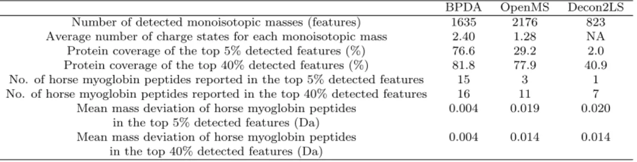
BPDA OpenMS Decon2LS Number of detected monoisotopic masses (features) 1635 2176 823 Average number of charge states for each monoisotopic mass 2.40 1.28 NA Protein coverage of the top 5% detected features (%) 76.6 29.2 2.0 Protein coverage of the top 40% detected features (%) 81.8 77.9 40.9 No. of horse myoglobin peptides reported in the top 5% detected features 15 3 1 No. of horse myoglobin peptides reported in the top 40% detected features 16 11 7 Mean mass deviation of horse myoglobin peptides 0.004 0.019 0.020
in the top 5% detected features (Da)
Mean mass deviation of horse myoglobin peptides 0.004 0.014 0.014 in the top 40% detected features (Da)
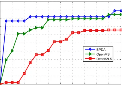
are summarized in Table III (we also considered the method implemented in the SpecArray package [29], but found it to be inferior to BPDA, OpenMS, and Decon2LS — the results were then omitted for the sake of conciseness). The number of features with unique monoisotopic masses detected by BPDA, OpenMS, and Decon2LS-Viper were 1635, 2176 and 823, respectively. In fact, it is not very informative to evaluate the performance of a detection algorithm solely based on the number of detected features, because of the presence of contaminants and false positive detections. Therefore, we focus on the top detected features yielded by each detection algorithm. Detected features were ranked by quality in descending order. Different algorithms utilize different quality metrics; for example, Decon2LS and OpenMS provide a quality score which measures how well an observed isotope pattern matches the predicted isotope pattern, while BPDA provides the peptide existence probability (see Eq. 2.26) as the quality measure. For each detection algorithm, for a given percentage of top detected features, we calculated the number of detected horse myoglobin peptides and the protein coverage rate. Note that by in-silico digestion of horse myoglobin, there are 39 tryptic peptides with less than 2 missed cleavage sites (19 of which do not contain any missed cleavage sites). Ideally, we should compare algorithms with known peptide composition in the sample and report protein coverage at different false positive rates. However, due to possible peptide contamination in the sample in any LC/MS experiment, actual peptide species presented in the sample are never known and this prevents us from estimating the false positive rates on the reported peptide list. As a result, the statistical significance of reported peptides by different peptide identification algorithms cannot be evaluated and the only option left for users in hope of obtaining a list of peptides with relatively low false positive rate is by applying a percentage threshold on the quality score reported by different algorithms. Thus, protein coverage v.s. percentage threshold on quality score is a meaningful
measurement of the performance of peak detection algorithms and the results are shown in Fig. 3. We need to point out that although the protein coverage of OpenMS seems to be comparable with the proposed algorithm in regions where the quality score percentage threshold is large, in such regions the reported peptide list may contain a lot of false positives and it is not an indication of good or bad algorithm performance. Instead, how quickly an algorithm reaches high protein coverage as the percentage threshold increases should be the measurement of the performance. In Fig. 3, we can see that BPDA reaches high protein coverage much faster than other algorithms at low percentage threshold regions.
0 10 20 30 40 50 60 70 80 90 100 0 10 20 30 40 50 60 70 80 90 100
Protein coverage results
Percentage of top detected features (%)
Protein coverage rate(%)
BPDA OpenMS Decon2LS
Fig. 3. Protein coverage results achieved by BPDA, OpenMS, and Decon2LS for the LC-MS data set MyoLCMS.
D. Discussion
We observed in our experiments that BPDA performs well on both simulated data and real data, for various SNRs and resolutions, and in complex cases where features overlap.
For the synthetic 20-mix experiment, we observe in Fig. 1 that the sensitivity (i.e., TPR) of BPDA was consistently higher than that of OpenMS for each abundance level, and both methods gave better sensitivity results as the abundance level (i.e., SNR) increased. Also it is observed that BPDA was quite robust for different SNRs. For the synthetic 10-mix experiment with overlapping peptides, we saw that BPDA detected all the peptides at a small false-positive rate F P R = 0.1, with very small mass deviations and quite accurate abundance results, and nearly all the charge states of the 10 true peptides were correctly reported. In contrast, atF P R= 0.1, OpenMS could detect only a few of the peptides. The abundance results given by OpenMS were not very close to those of the true peptides. Also OpenMS could only detect about half of the charge states.
The results obtained with real data corroborated the findings made with the syn-thetic experiments. For the MALDI-TOF MS 7-mix data, the four algorithms yielded similar intensity results, but BPDA was the only one to detect six out of the seven peptides. For the MyoLCMS experiment, we focused on protein coverage results, which is an important criterion to determine the confidence in protein identification and quantification [57, 58]. It was observed that BPDA displayed the largest protein coverage among the programs tested.