Statistics Publications Statistics
2011
A Semiparametric Estimation of Mean Functionals
With Nonignorable Missing Data
Jae Kwang Kim
Iowa State University, [email protected]
Cindy Long Yu
Iowa State University, [email protected]
Follow this and additional works at:http://lib.dr.iastate.edu/stat_las_pubs
Part of theDesign of Experiments and Sample Surveys Commons,Multivariate Analysis Commons, and theStatistical Methodology Commons
The complete bibliographic information for this item can be found athttp://lib.dr.iastate.edu/ stat_las_pubs/103. For information on how to cite this item, please visithttp://lib.dr.iastate.edu/ howtocite.html.
This Article is brought to you for free and open access by the Statistics at Iowa State University Digital Repository. It has been accepted for inclusion in Statistics Publications by an authorized administrator of Iowa State University Digital Repository. For more information, please contact
A semi-parametric estimation of mean
functionals with non-ignorable missing data
Jae Kwang Kim
Cindy Long Yu
∗Abstract
Parameter estimation with non-ignorable missing data is a challenging problem in statistics. The fully parametric approach for joint modeling of the response model and the population model can produce results that are quite sensitive to the failure of the assumed model. We propose a more robust modeling approach by considering the model for the nonresponding part as an exponential tilting of the model for the responding part. The exponential tilting model can be justified under the assumption that the response probability can be expressed as a semi-parametric logistic regression model.
In this paper, based on the exponential tilting model, we propose a semi-parametric estimation method of mean functionals with non-ignorable missing data. A semi-parametric logistic regression model is assumed for the response probability and a non-parametric regression approach for missing data discussed in Cheng (1994) is used in the estimator. By adopting nonparametric components for the model, the estimation method can be made robust. Variance estimation is also discussed and results from a simulation study are presented. The proposed method is applied to real income data from the Korean Labor and Income Panel Survey.
Key Words: Exponential tilting; Not missing at random; Nonparametric regression.
1
INTRODUCTION
Missing data is frequently encountered in many areas of statistics. Statistical analysis in the presence of missing data has been an area of considerable interest because ignoring the missing data often destroys the representativeness of the remaining sample and is likely to lead to biased parameter estimates. To account for the possible bias associated with missing data, statistical modeling is used to predict the missing part of the data. This type of modeling is challenging because it often depends on unverifiable assumptions. Finding a good prediction model is a crucial part of the missing data analysis.
In practice, the prediction model depends on an auxiliary variable. We assume that the auxiliary variable, x, is observed for the entire sample and only the study variable, y, is subject to missingness. In this setup, the usual approach is to find the best prediction model for y in terms of x. The prediction model can be used to predict the missing data if the response mechanism is ignorable in the sense that the relationship between y and x in the respondents also holds for the non-responding part of the sample. Nonresponse is ignorable if the study variable, y, is independent of the response status variable, r, conditional on the auxiliary variable x. Hence, it follows that nonresponse is non-ignorable if the probability of y being missing depends ony itself, even after controlling forx. This situation exists, for example, in surveys of income, where the nonresponse rates tend to be higher for low socio-economic groups. If nonresponse is non-ignorable, standard nonresponse adjustments such as stratification, reweighting, and imputation assuming an ignorable response mechanism will fail to correct for the bias due to nonresponse.
Parameter estimation for non-ignorable nonresponse data is a challenging problem be-cause the response mechanism is generally unknown and the parameters of the response probabilities need to be estimated. In the likelihood-based method, the fully parametric ap-proach involves joint modeling of the outcome and the response mechanism. Greenlees et al (1982) and Diggle and Kenward (1994) used explicit models for the response probability to
estimate the parameters. Baker and Laird (1988) and Ibrahim et al (1999) discussed maxi-mum likelihood estimation of the parameters under non-ignorable missing data based on the expectation-maximization algorithm. Molenberghs and Kenward (2007) provided a compre-hensive overview of the fully parametric approaches to the analysis of non-ignorable missing data. When the response mechanism is unknown, the identifiability of the parameters in the response mechanism is difficult to check. Chen (2001) and Tang et al (2003) discussed iden-tifiability conditions only under some limited situations. Furthermore, the fully parametric approach is very sensitive to failure of the assumed parametric models (Little, 1985).
In this paper, we propose a novel approach for modeling non-ignorable nonresponse based on the exponential tilting model, where the missing part of the data is modeled as an expo-nential tilt of the model for the responding part. The tilting parameter, which characterizes the tilt, determines the amount of departure from the ignorability of the response mecha-nism. The exponential tilting model for non-ignorable nonresponse is similar in spirit to the stratified Cox proportional hazards model considered in Scharfstein et al (1999), which was used to model non-ignorable drop-out in the analysis of longitudinal data. A semi-parametric logistic regression model with the tilting parameter is assumed for the response probability. The behavior of the non-responding part is estimated by using the nonparametric regression approach for missing data discussed by Cheng (1994). By adopting nonparametric parts for the model, the estimation method can be made more robust. Unlike Scharfstein et al (1999), we also consider the case where the tilting parameter is estimated, rather than known. Asymptotic normality, including the √n-consistency, of the proposed estimator is derived for the cases when the tilting parameter is estimated as well as known.
In Section 2, a basic setup is introduced. In Section 3, we propose a nonparametric estimation method with known tilting parameters and discuss some asymptotic properties. In Section 4, a semi-parametric estimation method using parametric estimates of tilting parameters is discussed. A simulation study and a case study are given in Section 5 and 6, respectively. Concluding remarks are made in Section 7.
2
BASIC SETUP
Let (xi, yi), i = 1,2,· · · , n, be n independent realizations of continuous random variables
(X, Y) from a distribution with joint distributionF (x, y), where xi is always observed and
yiis subject to missingness. We are interested in estimatingθ=E(Y). Letri be the original
response indicator for yi, where ri = 1 if yi is observed and ri = 0 otherwise. We assume
that the response mechanism is
ri |(xi, yi)∼Bernoulli(πi),
where πi =π(xi, yi), and ri is independent of rj for any i6=j. If πi does not depend on the
value ofyi, then the response mechanism is called ignorable.
Under the ignorable response mechanism or missing at random (MAR) condition, P r(yi ∈B |xi, ri = 0) =P r(yi ∈B |xi, ri = 1), (1)
for any measurable set B. Thus, under MAR, the conditional distribution of yi given xi
among the nonrespondents is the same as the conditional distribution among the respondents. Letf1(yi |xi) be the conditional density of yi given xi and ri = 1, and let f0(yi |xi) be the
conditional density of yi givenxi and ri = 0. Under MAR, we have f1(yi |xi) =f0(yi |xi),
and a consistent estimator of θ can be obtained by ˆ θ1 = 1 n n X i=1 {riyi+ (1−ri) ˆm(xi)}, (2)
where ˆm(xi) is a consistent estimator of m(xi) = E(yi |xi). The consistency of the
estima-tor (2) can be justified under the MAR condition.
If the MAR condition does not hold, then (1) does not hold and the estimator ˆθ1 in (2)
is biased. Instead, one can use ˆ θ2 = 1 n n X i=1 {riyi+ (1−ri) ˆm0(xi)},
where ˆm0(xi) is a consistent estimator of m0(xi) = E(yi |xi, ri = 0). In the absence of the
MAR condition, estimation of m0(xi) is difficult because yi is not observed in the set of
nonrespondents.
To compute the conditional distribution given ri = 0, we use the following relationship:
P r(yi ∈B |xi, ri = 0)
= P r(yi ∈B |xi, ri = 1)×
P r(ri = 0 |xi, yi ∈B)/P r(ri = 1|xi, yi ∈B)
P r(ri = 0|xi)/P r(ri = 1|xi)
. Thus, we can write the conditional distribution of the missing data given xas
f0(yi |xi) =f1(yi |xi)× O(xi, yi) E{O(xi, Yi)|xi, ri = 1} , (3) where O(xi, yi) = P r(ri = 0 |xi, yi) P r(ri = 1 |xi, yi) (4) is the conditional odds of nonresponse. The expression (3) is a basis for computing the conditional expectation, m0(xi) =E(yi |xi, ri = 0).
Assume that the response probability model is a logistic regression model π(xi, yi)≡P r(ri = 1|xi, yi) =
exp{g(xi) +φyi}
1 + exp{g(xi) +φyi}
(5) for some function g(·) and parameter φ. The response probability model (5) is a semi-parametric model in the sense that the component associated with xi, g(xi), is completely
unspecified and only the component associate with yi is parametrically modeled as φyi
with parameter φ. Under the response model (5), the odd function (4) can be written as O(xi, yi) = exp{−g(xi)−φyi} and the expression (3) can be simplified to
f0(yi |xi) =f1(yi |xi)×
exp (γyi)
E{exp (γYi)|xi, ri = 1}
, (6)
where γ =−φ. Model (6) states that the density for the nonrespondents is an exponential tilting of the density for the respondents. The parameter γ is the tilting parameter that
determines the amount of departure from the ignorability of the response mechanism. In risk theory literature (Gerber and Shiu, 1994), transformation (6) is often called Esscher transformation of f1(yi |xi) indexed by parameter γ.
In (3), we need two models to compute the conditional distribution of the nonrespondent: f1(yi |xi) andP r(ri = 1 |xi, yi). A consistent estimate off1(yi |xi), denoted by ˆf1(yi |xi),
can be non-parametrically estimated using a kernel estimator. Thus, in the exponential tilting model (6), the only parametric component that needs to be estimated is γ∗ = −φ∗, where φ∗ is the true value of φ in P r(ri = 1|xi, yi;φ∗) in (5). In some cases, such as with
planned missingness or a sensitivity analysis as described in Rotnitzky et al (1998), the parameter γ∗ is assumed to be known. In the other cases, the parameter γ∗ has to be estimated. To estimate the parameter, we often utilize a follow-up study where a further attempt is made to obtain responses in a subset of the nonrespondents. In Section 3, the theory is developed whenγ∗is known. In Section 4, we consider the case whenγ∗is estimated.
3
Nonparametric estimation
We first briefly discuss a nonparametric regression method for estimating m1(x) =
E(y|x, r= 1). Let K(·) be a symmetric density function on the real line and let h = hn
be a smoothing bandwidth such that hn → 0 and nhn → ∞ as n → ∞. The
nonparamet-ric regression estimator of m1(x) = E(y |x, r= 1) can be obtained by finding ˆm(x) that
minimizes Pn i=1riKh(xi, x){yi−m(x)}2 Pn i=1riKh(xi, x) , (7)
where Kh(u, x) = h−1K{(u−x)/h}. Note that (7) estimates the following quantity
Er{y−m(x)}2 |x=EE(y−m(x))2 |x, r= 1 |x. The function that minimizes (7) is
ˆ m1(x) = n X i=1 wi1(x)yi, (8)
where wi1(x) = riKh(xi, x) Pn j=1rjKh(xj, x) .
The weight wi1(x) in (8) represents the point mass assigned to yi when m1(x) is
approx-imated by Pn
i=1wi1(x)yi. The result of Devroye and Wagner (1980) can be used to show
that, under some regularity conditions, p lim n→∞ n X i=1 wi1(x)yi = E(rY |x) E(r|x) =E(Y |x, r= 1). (9)
Cheng (1994) proved√n-consistency of ˆθ1 in (2) with ˆm(x) = ˆm1(x) using the Kernel-based
regression estimator ˆm1(x) in (8) under ignorable missing data.
Under the non-ignorable missing setup described in Section 2 with an exponential tilt-ing model (6), if the true value γ∗ were known, the nonparametric regression estimator of m0(x) = E(y|x, r= 0) would be ˆ m0(x;γ∗) = n X i=1 wi0(x;γ∗)yi, (10)
where the weight
wi0(x;γ∗) = riKh(x, xi) exp(γ∗yi) Pn j=1rjKh(x, xj) exp(γ∗yj) = wi1(x) exp(γ ∗y i) Pn j=1wj1(x) exp(γ∗yj)
represents the point mass assigned toyi whenm0(x) is approximated by Pni=1wi0(x;γ∗)yi.
By the same argument for (9) ,
p lim n→∞ n X i=1 wi0(x)yi = E{rY exp (γ∗Y)|x} E{rexp (γ∗Y)|x} = E{π(x, Y)Y exp (γ ∗Y)|x} E{π(x, Y) exp (γ∗Y)|x} = E{(1−π(x, Y))Y |x} E{1−π(x, Y)|x} = E(Y |x, r= 0),
where π(x, y) = P r(r = 1|x, y). Using the nonparametric estimator ˆm0(x;γ∗) in (10), a
nonparametric estimator of θ =E(y) is computed by ˆ θN P = 1 n n X i=1 {riyi+ (1−ri) ˆm0(xi;γ∗)}. (11)
The following theorem, which is similar to Theorem 2.1 of Cheng (1994), presents some asymptotic properties of the estimator in (11). A sketch of the proof is presented in Appendix A.
Theorem 1 Assume that the response mechanism satisfies the semi-parametric response
model (5) with known parameter value φ∗. Under the regularity conditions described in Appendix A, the nonparametric estimator θˆN P in (11) with γ∗ =−φ∗ satisfies
√ n n ˆ θN P −θ o →N 0, σ12 (12) where σ2 1 =V(ηi) and ηi =m0(xi) + ri π(xi, yi) {yi−m0(xi)}. (13)
By Theorem 1, since ηi =yi +{ri/π(xi, yi)−1} {yi−m0(xi)}, we have
σ12 = V (Y) +E 1 π(X, Y) −1 (Y −m0(X))2 (14) and the increase in variance due to missing data is
V θˆN P −V θˆn = n−1E π(X, Y)−1−1 (Y −m0(X))2 ≥0, where ˆθn = n−1 Pn
i=1yi. The variance increase is determined by two factors: the inverse
of the response probability and the squared error term {Y −m0(X)}2. If the response
probabilities for some units are quite small, the variance increase can be quite large. If π(X, Y) does not depend on Y, σ2
1 in (14) reduces to σ12 =V (Y) +E 1 π(X)−1 V (Y |X) =V {E(Y |X)}+E 1 π(X)V (Y |X) , (15)
which is equal to the result of Cheng (1994). Thus, Theorem 1 is an extension of the result of Cheng (1994) to non-ignorable missing data. Wang and Rao (2002) also derived a result similar to (15).
To estimate the variance of the nonparametric estimator ˆθN P, we need to estimateσ12 in
(14). A consistent estimator of σ2 1 is ˆ σ21 = 1 n n X i=1 ˆ η2i − 1 n n X i=1 ˆ ηi !2 , (16) where ˆ ηi = ˆm0(xi;γ∗) + ri ˆ πi {yi−mˆ0(xi;γ∗)}, (17)
and ˆπi is the estimated response probability of (5) with known γ∗. Writing
α(x;γ∗) = O(x, y)/exp (γ∗y) = (π(x, y)−1−1) exp (−γ∗y), where O(x, y) is defined in (4), we have
E{rO(x, Y)|x}=E(1−r|x) =α(x;γ∗)E{rexp (γ∗y)|x}.
Thus, under the semi-parametric logistic regression model (5) with known parameter γ∗ = −φ∗, a non-parametric estimator of π
i =π(xi, yi) can be obtained by ˆπi = ˆπi(γ∗), where
ˆ πi(γ) ={1 + ˆα(xi;γ) exp (γyi)} −1 , (18) and ˆ α(xi;γ) = Pn j=1(1−rj)Kh(xi, xj) Pn j=1rjexp (γyj)Kh(xi, xj) .
The non-parametric estimator ˆπi in (18) can be used to compute the pseudo-value ˆηi
in (17). Note that the use of ˆηi = ˆm0(xi;γ∗) +ri{yi−mˆ0(xi;γ∗)} is equivalent to the
naive variance estimator, which is well known to underestimate the variance. The inflation factor ˆπi−1 in the residual part of ˆηi properly reflects the increase of variance due to missing
data. The pseudo-values in (17) bear the same form as those in Carpenter, Kenward and Vansteelandt (2006) under ignorable missing, and are also used for variance estimation in Kim and Rao (2009).
4
Semi-parametric estimation
In many cases, tilting parameter γ∗ is unknown and has to be estimated. We now consider a semi-parametric estimator of θ in the sense that we use a parametric component ˆγ for the nonparametric estimation ofm0(x;γ) = E(Y |x, r= 0;γ). We consider two scenarios. The
first scenario is the case when the parameter estimate forγ∗ is computed from an independent survey. The second scenario is when the parameter estimate is obtained from a validation sample, which is a subsample of the nonrespondents.
In either case, the resulting semi-parametric estimator of θ is ˆ θSP = 1 n n X i=1 {riyi+ (1−ri) ˆm0(xi; ˆγ)}, (19)
where ˆm0(xi;γ) is defined in (10). We first consider the scenario where ˆγ is estimated from
an independent survey. The following theorem presents some asymptotic properties of the proposed estimator in (19) for this scenario. A sketch of the proof is in Appendix B.
Theorem 2 Assume that the conditions of Theorem 1 hold, except that φ∗ in the response
model (5) is known. Let θˆSP be the semi-parametric estimator constructed in (19) for the
marginal mean of y with ˆγ satisfying
√
n(ˆγ−γ∗)→N(0, Vγ), (20)
and assume that γˆ is independent of θˆN P in (11).
Then, we have √ n(ˆθSP −θ)→N(0, σ22), (21) where σ22 =σ12+H2Vγ, (22) H=E(1−r) (Y −m0(X))2 , and σ12 is defined in (14).
Note that if ˆγ is exactly estimated, then Vγ = 0 andσ22 is equal toσ12. Thus, the second
term in (22), the increase in variance, is the cost from estimatingγ. A consistent estimator of σ2
2 is
ˆ
σ22 = ˆσ12+ ˆH2Vˆγ,
where ˆσ1 is computed using (16), ˆVγ is a consistent estimator of nV (ˆγ), and
ˆ H = 1 n n X i=1 (1−ri) ˆσ02(xi), with ˆ σ02(xi) = Pn j=1rjKh(xi, xj) exp (ˆγyj) (yj −mˆ0(xj))2 Pn j=1rjKh(xi, xj) exp (ˆγyj) .
A consistent estimator of σ21 using (16) can be computed by using the pseudo values ˆ ηi = ˆm0(xi; ˆγ) + ri ˆ πi(ˆγ) {yi−mˆ0(xi; ˆγ)}, where ˆπi(γ) is defined in (18).
We now consider the case when a validation sample is randomly selected from the set of nonrespondents and the responses are obtained for all the elements in the validation sample. A consistent estimator ˆγ of γ∗ can be obtained by solving
n
X
i=1
(1−ri)δi{yi−mˆ0(xi;γ)}= 0, (23)
for γ, where δi is an indicator function that takes the value one if unit i belongs to the
follow-up sample and takes the value zero otherwise,and ˆm0(xi;γ) is defined in (10).
Using the estimated tilting parameter ˆγ obtained from (23), one can construct ˆθSP in
(19). The following theorem presents some asymptotic properties of the estimators using the estimated tilting parameter obtained from (23). A sketch of the proof is in Appendix C.
Theorem 3 Assume that the conditions of Theorem 1 hold, except for the semi-parametric
ˆ
θSP be the semi-parametric estimator constructed in (19) for the marginal mean of y using
ˆ
γ obtained by solving (23). Then, we have
√ n(ˆθSP −θ)→N(0, σ23) (24) where σ2 3 =V(η2i), η2i = ˜m(xi;γ0) + δi ν(1−ri) +ri {yi−m˜(xi;γ0)}, ˜
m(x;γ) = plimn→∞mˆ0(x;γ), ν =E(δ|r= 0) and γ0 is the probability limit of γˆ.
In Theorem 3, the response model (5) is not needed to show the result (24). The variance σ2
3 can be written
σ23 =V(Y) + ν−1 −1E(1−r){y−m˜(x;γ0)}2
. Thus, in the extreme case of ν = 1, we haveσ2
3 =V(Y). Note that ˜ m(x;γ) =p lim n→∞ Pn j=1Kh(x, xj)rjexp(γyj)yj Pn j=1Kh(x, xj)rjexp(γyj) = E{rexp (γY)Y |x} E{rexp (γY)|x} . Thus, if the response model (5) is true, then γ0 =γ∗ and, by (24),
˜ m(x;γ0) = E{rexp (γ∗Y)Y |x} E{rexp (γ∗Y)|x} = E{(1−r)Y |x} E{(1−r)|x} =E(Y |x, r = 0) =m0(x). Since E (1−r){y−m˜(x;γ0)}2 ≥E (1−r){y−m0(x)}2 ,
the variance σ32 in (24) is minimized when the assumed response model (5) is true. Thus, the validity of the proposed estimator does not depend on the assumed response model and the role of the response model (5) is to improve the efficiency.
For variance estimation, a consistent estimator of σ2 3 is ˆ σ23 = 1 n n X i=1 ˆ η22i− 1 n n X i=1 ˆ η2i !2 ,
where ˆ η2i = ˆm0(xi; ˆγ) + δi ν (1−ri) +ri {yi−mˆ0(xi; ˆγ)}.
Instead of using ˆθSP in (19), one can use the observed valuesyi from both the respondents
and the follow-up samples directly to get ˆ θSP2 = 1 n n X i=1 {riyi+ (1−ri)δiyi+ (1−ri) (1−δi) ˆm0(xi; ˆγ)}. (25) By (23), we have ˆ θSP2 = 1 n n X i=1 {riyi+ (1−ri) ˆm0(xi; ˆγ)}= ˆθSP.
Thus, the extra information in the follow-up sample is fully incorporated in ˆθSP and there
is no efficiency gain in using ˆθSP2.
5
Simulation Study
To test our theory, we performed a simulation study. In the simulation, we considered two models for generating (xi, yi). In model A, the sample of (xi, yi) is generated from
xi ∼N(2,1) and yi = 1 + 0.7xi+ei whereei ∼N(0,1). In model B, (xi, ei) are the same as
in model A but yi = 1 + 0.5(x−2.5)2+ei. In addition to (xi, yi), we also generated ri, the
response indicator variable, from Bernoulli distributions with probability πi. We considered
eight response models for πi:
(M1): (Linear Ignorable)
πi =
exp(φ0+φ1xi)
1 + exp(φ0+φ1xi)
, where (φ0, φ1) = (−1.5,1.0) for both models.
(M2): (Linear Non-ignorable) πi =
exp(φ0 +φ1xi+φ2yi)
1 + exp(φ0+φ1xi+φ2yi)
where (φ0, φ1, φ2) = (−0.85,0.3,0.3) for model A and (φ0, φ1, φ2) = (−1.58,0.5,0.7)
for model B.
(M3): (Non-linear Non-ignorable: quadratic in x) πi =
exp(φ0+φ1xi+φ2x2i +φ3yi)
1 + exp(φ0+φ1xi+φ2x2i +φ3yi)
,
where (φ0, φ1, φ2, φ3) = (−2.0,0.3,0.3,0.3) for model A and (φ0, φ1, φ2, φ3) =
(−2.72,2.72,−0.68,0.7) for model B. (M4): (Jump Non-ignorable)
πi = 0.5 if yi ≤c
= 1.0 if yi > c
, where c= 3.4 for model A and c= 2.5 for model B. (M5): (Non-linear Non-ignorable: quadratic in y)
πi =
exp(φ0+φ1xi+φ2yi+φ3yi2)
1 + exp(φ0+φ1xi+φ2yi+φ3y2i)
,
where (φ0, φ1, φ2, φ3) = (−0.65,0.1,0.1,0.1) for model A and (φ0, φ1, φ2, φ3) =
(−0.85,0.1,0.1,0.3) for model B. (M6): (Probit Non-ignorable)
πi = Φ(φ0+φ1xi+φ2yi),
where Φ(·) is the cumulative density function of the standard normal distribution, (φ0, φ1, φ2) = (−0.64,0.1,0.3) for model A and (φ0, φ1, φ2) = (−0.53,0.1,0.4) for model
B.
(M7): (Complementary log-log Non-ignorable)
πi = 1−exp{−exp(φ0+φ1xi+φ2yi)},
where (φ0, φ1, φ2) = (−1.4,0.3,0.3) for model A and (φ0, φ1, φ2) = (−1.15,0.3,0.3) for
(M8): (Non-linear Non-ignorable: interaction) πi =
exp(φ0+φ1xi+φ2yi +φ3xiyi)
1 + exp(φ0+φ1xi+φ2yi+φ3xiyi)
,
where (φ0, φ1, φ2, φ3) = (−1.4,0.1,0.1,0.3) for model A and (φ0, φ1, φ2, φ3) =
(−0.15,0.1,0.1,0.1) for model B.
The missing scenarios considered above include one ignorable missing case (M1) and seven different kinds of non-ignorable missing cases (M2)-(M8). The response rates are about 60% in every combination of the two models and eight response mechanisms. Scenarios (M1)-(M3) satisfy the response probability assumption in (5). Missing mechanisms (M4)-(M8), which do not satisfy (5), were included to examine the robustness of our semi-parametric estimators against failure of the assumed missing mechanism.
For each combination of the two models and eight missing scenarios above, Monte Carlo samples of size n = 200 were independently generated B = 2,000 times. In each of the sixteen samples, we computed four point estimators:
1. ˆθn =n−1Pni=1yi: sample mean of y. Note that ˆθn is not used in practice because yi is
not available for ri = 0.
2. ˆθN A =n−1
Pn
i=1{riyi + (1−ri) ˜m0(xi)}: a naive estimator where
˜ m0(x) = Pn i=1(1−ri)δiKh(x, xi)yi Pn i=1(1−ri)δiKh(x, xi) , using only the follow-up data.
3. ˆθ1: Cheng’s estimator in (2) with ˆm(x) = ˆm1(x) in (8). ˆθ1 assumes that missing data
from the response mechanism are ignorable.
4. ˆθSP: the semi-parametric estimator in (19) using the estimated tilting parameter ˆγ
The nonparametric Kernel regression estimator was computed using a Gaussian kernel function with bandwidthh = ˆσxn−1/5, where ˆσx is the estimated standard deviation of xi in
the sample. The estimated tilting parameter ˆγ was computed by solving the equation (23) using a Newton-Raphson method.
<Table 1 around here. > <Table 2 around here. >
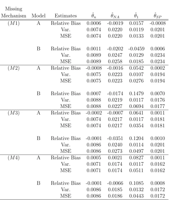
Table 1 and Table 2 present the Monte Carlo relative biases and variances of the four point estimators computed from the Monte Carlo samples of sizeB = 2,000 for missing cases (M1)-(M4) and (M5)-(M8) separately. Mean squared errors (MSE) are reported as well.
Comparing our semi-parametric estimator ˆθSP to Cheng’s estimator ˆθ1, we found that
(i) under the ignorable missing mechanism (M1), although the relative biases in ˆθSP are
smaller than those in Cheng’s estimator, Cheng’s estimator has better performance in terms of MSE since the missing mechanism is correctly specified; (ii) under all the non-ignorable missing mechanisms (M2)-(M8), Cheng’s estimator as expected is much more seriously biased than our semi-parametric estimator because Cheng’s estimator incorrectly assumes that the response mechanism is ignorable. Although our semi-parametric estimator loses some efficiency due to estimating ˆγ, the serious biases in Cheng’s lead to much bigger MSE under all the non-ignorable missing cases.
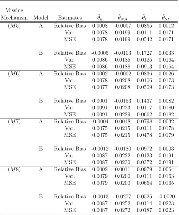
When comparing our semi-parametric estimator ˆθSP to the naive estimator ˆθN A, we found
that under all the circumstances our semi-parametric estimator performs better than the naive estimator in terms of efficiency and MSE. The efficiency gain in the semi-parametric estimator may be ascribed to the fact that in our semi-parametric estimator the respondent data is used for estimating m0(x), while the naive estimator utilizes only the follow-up data
to estimate m0(x). It is also noteworthy that our semi-parametric estimator consistently
are wrong, i.e. (M4)-(M8). This robustness property is consistent with our finding in Theo-rem 3 that the validity of the proposed estimator does not depend on the assumed response model.
6
Empirical Study
In this section, the proposed semi-parametric estimators are applied to the Korea Labor and Income Panel Survey (KLIPS). A brief description of the panel survey can be found at http://www.kli.re.kr/klips/en/about/introduce.jsp. The data consist of n = 2,506 regular wage earners from the year 2008 sample. The study variable (y) is the average monthly income for the current year and the auxiliary variable (x) is the average monthly income for the previous year. The sample mean of (x, y) is (1.6643,1.8504)×106 Korean Won and the
sample correlation between x and y is 0.8144.
From the sample described above, we created artificial missing data by deliberately deleting some of the y values according to the eight response models defined in Section 5. Specifically, we used (φ0, φ1) = (−1.13,1.0) for (M1), (φ0, φ1, φ2) = (−1.5,0.5,0.7) for
(M2), (φ0, φ1, φ2, φ3) = (−2.15,0.2,0.5,0.7) for (M3), c = 2.5 for (M4), (φ0, φ1, φ2, φ3) =
(−0.65,0.1,0.1,0.2) for (M5), (φ0, φ1, φ2) = (−0.41,0.1,0.3) for (M6), (φ0, φ1, φ2) =
(−1.42,0.1,0.7) for (M7), and (φ0, φ1, φ2, φ3) = (−0.78,0.1,0.1,0.3) for (M8). Each of the
eight response mechanisms with the specified parameter values above produced about 60% response rates. Among the nonrespondents, 15% were randomly selected for follow-up sam-ples. Thus, from the original data with sample size of n = 2,506, we have about 1,504 respondents and 150 people who responded to the follow-up. Cheng’s estimator ˆθ1 and our
semi-parametric estimator ˆθSP were computed using the real data with the artificial missing
values for each response probability model.
<Table 3 around here. >
b
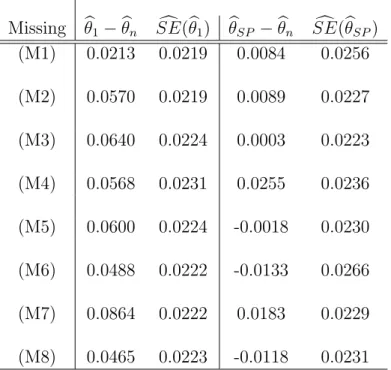
θn = 1.8504 and the estimated standard errors of the point estimators for each of the missing
mechanisms. We used the variance estimation formula for ˆθSP from Section 4 and the
esti-mated variance of ˆθ1 was computed following the approach in Cheng (1994). The estimated
mean errors θb1 −bθn based on Cheng’s estimator are consistently larger in magnitude than b
θSP −θbn based on our semi-parametric estimator under all the missing scenarios, including the missing ignorable case (M1). This case study demonstrates the empirical effectiveness of our semi-parametric estimator.
7
Conclusion
In the presence of missing data, estimation of θ =E(y) involves computing the conditional expectation E(yi | xi, ri = 0). When the response mechanism is ignorable, Cheng (1994)
considered using a nonparametric estimator, m1(xi) = E(yi |xi, ri = 1), for E(yi | xi, ri =
0). If the response mechanism is not ignorable, then the exponential tilting model (6) can be used to derive a consistent estimator of m0(xi) =E(yi |xi, ri = 0). If the tilting parameter
γ∗ is known in advance, a non-parametric estimator of m0(xi) can be obtained by ˆm0(xi;γ∗)
in (10). When the tilting parameter γ∗ is unknown, an estimating equation (23) can be used to obtain ˆγ, which can be used to construct semi-parametric estimators in (19) and in (25). The asymptotic properties and the simulation and empirical results presented in this paper show that the semi-parametric estimator provides satisfactory performances in general. Extension to other parameters, such as the population variance, can follow naturally. Extension of the theorems to cases where xis ad-dimensional vector, which is not discussed in this paper, can also be made by choosing the bandwidth nhd → ∞ instead of nh→ ∞. However, as with any nonparametric kernel method, the proposed semi-parametric method can show poor performance for the samples with small sizes or with some extreme missing data patterns.
com-plete response among the elements in the validation subsample. If there is still missingness in the validation subsample, the estimating equation (23) cannot be used to estimateγ∗ and the proposed method is not applicable. In this case, a prior belief about γ∗ can be used, as (20), using a Bayesian argument. Investigation of alternative methods for estimating γ∗, including the Bayesian approach, is a topic for future research.
Acknowledgments
We thank two anonymous referees and the associate editor for very helpful comments. The research was partially supported by Cooperative Agreement No. 68-3A75-4-122 between the USDA Natural Resources Conservation Service and the Center for Survey Statistics and Methodology at Iowa State University.
References
Baker, S. G. and N. M. Laird (1988). Regression analysis for categorical variables with outcome subject to nonignorable nonresponse. Journal of the American Statistical Asso-ciation 83, 62-69.
Carpenter, J.R., Kenward, M. G. and Vansteelandt, S. (2006). A Comparison of Multiple Imputation and Doubly Robust Estimation for Analyses with Missing Data. Journal of the Royal Statistical Society, Series A 169, 571-584.
Chen, K. (2001). Parametric models for response-biased sampling. Journal of the Royal Statistical Society, Series B 63, 775-789.
Cheng, P.E. (1994). Nonparametric estimation of mean functionals with data missing at random. Journal of the American Statistical Association 89, 81-87.
Devroye, L.P. and Wagner, T.J. (1980). Distribution-free consistency results in nonpara-metric discrimination and regression function estimations, The Annals of Statistics 8, 231-239.
Diggle, P. and Kenward, M.G. (1994). Informative drop-out in longitudinal data analysis (with discussion), Applied Statistics 42, 105-115.
Gerber, H.U. and Shiu, E.S.W. (1994). Option Pricing by Esscher Transforms,Transactions of the Society of Actuaries, 46, pp. 99191.
Greenlees, W.S., Reece, J.S., and Zieschang, K.D. (1982). Imputation of missing values when the probability of response depends on the variable being imputed, Journal of the American Statistical Association 77, 251–261.
Ibrahim, J.G., Lipsitz, S.R., and Chen, M. (1999). Missing covariates in generalized linear models when the missing data mechanism is non-ignorable,Journal of the Royal Statistical Society: Series B 61, 173-190.
Kim, J.K. and Rao, J.N.K. (2009). Unified approach to linearization variance estimation from survey data after imputation for item nonresponse, Biometrika,96, 917-932.
Little, R.J.A. (1985). A note about models for selectivity bias,Econometrica 53, 1469-1474. Molenberghs, G. and Kenward, M.G. (2007). Missing data in clinical studies, John Wiley &
Sons: Chichester.
Randles, R. H. (1982). On the asymptotic normality of statistics with estimated parameters.
The Annals of Statistics 10, 462-474.
Rotnitzky, A., Robins, J. and Scharfstein, D. (1998). Semiparametric regression for repeated outcomes with non-ignorable non-response. Journal of the American Statistical Associa-tion 93, 1321-1339.
Scharfstein D.O., Rotnitzky A., Robins J.M. (1999). Adjusting for nonignorable drop-out using semiparametric nonresponse models (with discussion). Journal of the American Statistical Association 94, 1096-1120.
Tang, G., Little, R.J.A., and Raghunathan, T.E. (2003). Analysis of multivaraite missing data with nonignorable nonresponse. Biometrika 90, 747-764.
Wang, Q. and Rao, J.N.K. (2002). Empirical likelihood-based inference under imputation for missing response data. Annals of Statistics 30, 896-924.
Appendix
A: Proof of Theorem 1
Before deriving the asymptotic limit of ˆθ, we need the following regularity conditions. (C.1) The kernel functionK(w) is a probability density function such that
(i) it is bounded and has compact support; (ii) it is symmetric with σ2
k=
R
w2K(w)dw <∞;
(iii) K(w)≥d1 for somed1 >0 in some closed interval centered at zero.
(C.2) nh→ ∞ and nh4 →0.
(C.3) E[y2] and E[exp(2γ∗y)] are finite. (C.4)
(i)π(x, y)> d2 >0 and p(x) = E[π(x, y)|x]6= 1 almost surely.
(ii) The density of X decays exponentially fast.
(iii) m0(x) has bounded second derivative and satisfies
E[exp(γ∗y)|m00(x)α0(x) + 0.5m000(x)α(x)|]<∞, where α(x) =O(x, y)/exp(γ∗y).
Proof: Write
ˆ
where A = n−1 n X i=1 {rim1(xi) + (1−ri)m0(xi)} (A.2) B = n−1 n X i=1 ri{yi−m1(xi)} (A.3) C = n−1 n X i=1 (1−ri){mˆ0(xi)−m0(xi)}.
By the classical central limit theorem, √n(A−θ) converges to the normal distribution with mean 0 and variance V {rm1(x) + (1−r)m0(x)}. The term
√
nB converges to the normal distribution with mean 0 and variance
Er(Y −m1(X)) 2
=Eπ(X, Y) (Y −m1(X)) 2
. For the C term, note that we can write
C=n−1 n X i=1 (1−ri) Pn j=1rjexp (γ ∗ yj)Kh(xj, xi){yj −m0(xi)} Pn j=1rjexp (γ∗yj)Kh(xj, xi) (A.4) and p lim n→∞ Pn j=1rjexp (γ∗yj)Kh(xj, x) Pn j=1Kh(xj, x) = E{rexp (γ∗Y)|x} = E[rO(x, Y) exp{g(x)} |x] = {1−p(x)}exp{g(x)}, where O(x, y) is defined in (4) and p(x) =E(r |x). Thus,
p lim n→∞ 1 n n X j=1 rjexp (γ∗yj)Kh(xj, x) = f(x){1−p(x)}exp{g(x)},
wheref(x) is the marginal density ofX. Using the same argument for Theorem 2.1 of Cheng (1994), it can be shown that
√
where C∗ =n−1 n X j=1 rjexp (γ∗yj){yj−m0(xj)}α(xj) and α(xj) = E (1−r)Kh(x, xj){1−p(x)} −1 exp{−g(x)}f−1(x)|xj = exp{−g(xj)}.
Thus, we can write
C∗ = n−1 n X j=1 rjO(xj, yj){yj −m0(xj)} = n−1 n X j=1 rj 1 π(xj, yj) −1 {yj−m0(xj)}.
Thus, inserting (A.5) into (A.1), we have √
nnθˆN P −(A+B+C∗)
o
=op(1).
Note thatA+B+C∗ = ¯ηn,where ¯ηn=n−1
Pn
i=1ηiwithηiin (13). Sinceηi are independently
and identically distributed with mean E(ηi) = θ, we have
√
n(¯ηn−θ)→N 0, σ21
and (12) follows by the Slutsky theorem.
B: Proof of Theorem 2
Proof: Using the argument similar to the proof of Theorem 1,
ˆ
θSP =A+B+C∗ +W +op n−1/2
, (A.6)
where A, B, and C∗ are defined in (A.2), (A.3), and (A.6), respectively, and W = n−1Pn i=1(1−ri)[ ˆm0(xi; ˆγ)−mˆ0(xi;γ∗)]. By a Taylor expansion, W = (ˆγ−γ∗)01 n n X i=1 (1−ri) ∂mˆ0(xi;γ1) ∂γ ,
where ∂mˆ0(xi;γ) ∂γ = Pn j=1rjKh(xi, xj) exp(γyj)y 2 j Pn j=1rjKh(xi, xj) exp(γyj) −mˆ20(xi;γ),
and γ1 is in the line segment between ˆγ and γ∗. Standard arguments used to derive the
asymptotic equivalence (A.5) can also be used to show that, as n → ∞, 1 n n X i=1 (1−ri) ∂mˆ0(xi;γ1) ∂γ →p E[(1−r){y−m0(x)} 2|x ]. (A.7)
Hence,W is asymptotically equivalent to (ˆγ−γ)E[(1−r){y−m0(x)}2] and
√
nW converges to N(0, H2V
γ). Due to the independence of ˆγ, W is uncorrelated with (A, B, C∗) and the
result (21) follows.
C: Proof of Theorem 3
Proof: Writing ˆ θSP (γ) = 1 n n X i=1 {riyi+ (1−ri) ˆm0(xi;γ)}+ 1 n n X i=1 (1−ri) δi ν {yi−mˆ0(xi;γ)}, we have ˆθSP(ˆγ) = ˆθSP and E ∂ ∂γ ˆ θSP (γ)|γ =γ0 = 0 (A.8)where γ0 is the probability limit of ˆγ. According to Randles (1982), using
√ n(ˆγ−γ0) = Op(1), we have ˆ θSP (ˆγ) = ˆθSP(γ0) +op(n−1/2). (A.9) Writing ˜ m(x;γ) =p lim n→∞mˆ0(x;γ) = E{rexp (γY)Y |x} E{rexp (γY)|x} , we have ˆ θSP(γ0) = n−1 n X i=1 {riyi + (1−ri) ˜m(x;γ0)}+n−1 n X i=1 (1−ri) δi ν {yi−m˜(x;γ0)}+U(γ0),
where U(γ0) = n−1 n X i=1 (1−ri) (1−δi/ν){mˆ0(xi;γ0)−m˜(xi;γ0)}. Because ˆ m0(xi;γ0)−m˜(xi;γ) = Pn j=1rjKh(xi, xj) exp(γ0yj){yj −m˜(xi;γ0)} Pn j=1rjKh(xi, xj) exp(γ0yj) ,
we can apply the same argument for (A.5) to the last term of U(γ0) to get
√ n{U(γ0)−U∗(γ0)}=op(1), (A.10) where U∗(γ0) =n−1 n X i=1 riexp(γ0yi){yi−m˜(xi;γ0)}α∗(xi) and α∗(xi) = E{(1−r) (1−δ/ν)Kh(x, xi)|xi} f(xi)E{rexp(γ0Y)|xi} .
BecauseE{δ |r= 0, x}=ν,α∗(xi) = 0 and (A.10) reduces toU(γ0) =op(n−1/2). Therefore,
(A.9) reduces to ˆ θSP =n−1 n X i=1 {riyi+ (1−ri) ˜m(x;γ0)}+n−1 n X i=1 (1−ri) δi ν {yi−m˜(x;γ0)}+op(n −1/2), which proves (24).
Table 1: Monte Carlo relative biases, Monte Carlo variances, and Monte Carlo mean squared errors of the four point estimators for missing scenarios (M1)-(M4) in the simulation study.
Missing
Mechanism Model Estimates θˆn θˆN A θˆ1 θˆSP
(M1) A Relative Bias 0.0006 -0.0019 0.0157 -0.0008 Var. 0.0074 0.0220 0.0119 0.0201 MSE 0.0074 0.0220 0.0133 0.0201 B Relative Bias 0.0011 -0.0202 -0.0459 0.0006 Var. 0.0089 0.0247 0.0129 0.0234 MSE 0.0089 0.0258 0.0185 0.0234 (M2) A Relative Bias -0.0008 -0.0016 0.0542 0.0002 Var. 0.0075 0.0223 0.0107 0.0194 MSE 0.0075 0.0223 0.0276 0.0194 B Relative Bias 0.0007 -0.0174 0.1479 0.0070 Var. 0.0088 0.0219 0.0117 0.0176 MSE 0.0088 0.0227 0.0694 0.0177 (M3) A Relative Bias -0.0002 -0.0007 0.0641 0.0011 Var. 0.0074 0.0217 0.0117 0.0181 MSE 0.0074 0.0217 0.0354 0.0181 B Relative Bias -0.0001 -0.0351 0.1204 0.0010 Var. 0.0086 0.0240 0.0114 0.0201 MSE 0.0086 0.0273 0.0497 0.0201 (M4) A Relative Bias 0.0005 0.0021 0.0827 0.0011 Var. 0.0071 0.0174 0.0117 0.0162 MSE 0.0071 0.0174 0.0511 0.0162 B Relative Bias -0.0001 -0.0066 0.1085 0.0008 Var. 0.0086 0.0185 0.0132 0.0172 MSE 0.0086 0.0186 0.0443 0.0172
Table 2: Monte Carlo relative biases, Monte Carlo variances, and Monte Carlo mean squared errors of the four point estimators for missing scenarios (M5)-(M8) in the simulation study.
Missing
Mechanism Model Estimates θˆn θˆN A θˆ1 θˆSP
(M5) A Relative Bias 0.0008 -0.0007 0.0865 0.0012 Var. 0.0078 0.0199 0.0111 0.0171 MSE 0.0078 0.0199 0.0542 0.0171 B Relative Bias -0.0005 -0.0103 0.1727 0.0033 Var. 0.0086 0.0185 0.0125 0.0164 MSE 0.0086 0.0188 0.0913 0.0164 (M6) A Relative Bias 0.0002 -0.0002 0.0836 0.0026 Var. 0.0078 0.0208 0.0106 0.0173 MSE 0.0077 0.0208 0.0509 0.0173 B Relative Bias 0.0001 -0.0153 0.1437 0.0082 Var. 0.0091 0.0223 0.0117 0.0180 MSE 0.0091 0.0229 0.0662 0.0182 (M7) A Relative Bias -0.0004 0.0018 0.0798 0.0032 Var. 0.0075 0.0215 0.0111 0.0178 MSE 0.0075 0.0215 0.0478 0.0179 B Relative Bias -0.0012 -0.0180 0.0972 0.0003 Var. 0.0087 0.0222 0.0123 0.0191 MSE 0.0087 0.0230 0.0372 0.0191 (M8) A Relative Bias 0.0002 0.0011 0.0979 0.0064 Var. 0.0079 0.0200 0.0111 0.0163 MSE 0.0079 0.0200 0.0664 0.0165 B Relative Bias -0.0013 -0.0277 0.0525 -0.0020 Var. 0.0087 0.0252 0.0114 0.0223 MSE 0.0087 0.0272 0.0187 0.0223
Table 3: Estimated mean errors and estimated standard errors for the Cheng’s estimator (ˆθ1) and our semi-parametric estimator (ˆθSP) in the case study.
Missing bθ1−θbn SEc(θb1) θbSP −θbn SEc(bθSP) (M1) 0.0213 0.0219 0.0084 0.0256 (M2) 0.0570 0.0219 0.0089 0.0227 (M3) 0.0640 0.0224 0.0003 0.0223 (M4) 0.0568 0.0231 0.0255 0.0236 (M5) 0.0600 0.0224 -0.0018 0.0230 (M6) 0.0488 0.0222 -0.0133 0.0266 (M7) 0.0864 0.0222 0.0183 0.0229 (M8) 0.0465 0.0223 -0.0118 0.0231