Demiris, Nikolaos (2004) Bayesian Inference for
Stochastic Epidemic Models using Markov chain Monte
Carlo Methods. PhD thesis, University of Nottingham.
Access from the University of Nottingham repository: http://eprints.nottingham.ac.uk/10078/1/Thesis.pdf
Copyright and reuse:
The Nottingham ePrints service makes this work by researchers of the University of Nottingham available open access under the following conditions.
· Copyright and all moral rights to the version of the paper presented here belong to the individual author(s) and/or other copyright owners.
· To the extent reasonable and practicable the material made available in Nottingham ePrints has been checked for eligibility before being made available.
· Copies of full items can be used for personal research or study, educational, or not-for-profit purposes without prior permission or charge provided that the authors, title and full bibliographic details are credited, a hyperlink and/or URL is given for the original metadata page and the content is not changed in any way.
· Quotations or similar reproductions must be sufficiently acknowledged.
Please see our full end user licence at:
http://eprints.nottingham.ac.uk/end_user_agreement.pdf
A note on versions:
The version presented here may differ from the published version or from the version of record. If you wish to cite this item you are advised to consult the publisher’s version. Please see the repository url above for details on accessing the published version and note that access may require a subscription.
Bayesian Inference for Stochastic Epidemic Models
using Markov chain Monte Carlo Methods
by Nikolaos Demiris, BSc, MSc
Thesis submitted to the University of Nottingham
for the degree of Doctor of Philosophy, January 2004
Contents
1 Introduction to Stochastic Epidemic Models, Bayesian
Statis-tics and Inference from Outbreak Data 1
1.1 Introduction . . . 1
1.1.1 Epidemic Modelling . . . 2
1.1.2 Bayesian Inference . . . 4
1.1.3 Inference from Outbreak Data using Epidemic Models . . 6
1.2 Stochastic Epidemic models . . . 7
1.2.1 Generalised Stochastic Epidemic model . . . 7
1.2.2 Epidemic models with two levels of mixing . . . 11
1.3 Bayesian Statistical Inference . . . 15
1.3.1 Basic theory . . . 15
1.3.2 Bayesian Computation . . . 20
1.4 Statistical Inference from Outbreak Data . . . 25
1.4.1 The Nature of Infectious Disease Data . . . 25
1.4.2 Previous Work on Epidemic Modelling . . . 27
2 Exact Results for the Generalised Stochastic Epidemic 34 2.1 Introduction . . . 34
2.2 The Generalised Stochastic Epidemic . . . 36
2.2.1 The Basic Model . . . 36
2.2.2 Final Size Probabilities . . . 37
2.3 Exact Final Size Probabilities . . . 39
2.3.1 Multiple Precision Arithmetic . . . 39
2.3.2 Multiple Precision Final Size Probabilities . . . 40
2.4 Evaluation of limit theorems . . . 41
2.4.1 Probability of Epidemic Extinction . . . 41
2.4.2 Gaussian Approximation . . . 43
2.5 Statistical Inference for the GSE . . . 47
2.5.1 Bayesian Inference . . . 47
2.5.2 MCMC algorithm . . . 48
2.6 Results . . . 49
2.7 Conclusion . . . 56
3 Approximate Bayesian Inference for Epidemics with two levels of mixing 57 3.1 Introduction . . . 57
3.2 Epidemic models with two levels of mixing . . . 58
3.2.1 Stochastic Epidemic model . . . 58
3.2.2 Final outcome of a homogeneous SIR epidemic with out-side infection . . . 59
3.2.3 Asymptotic approximations . . . 62
3.3 Data and Augmented Likelihood . . . 67
3.3.2 Augmented Likelihood . . . 68
3.4 Markov chain Monte Carlo algorithm . . . 70
3.5 Application to data . . . 72
3.5.1 Influenza outbreak data . . . 72
3.5.2 Artificial final outcome data . . . 82
3.5.3 Simulated final outcome data . . . 86
3.6 Evaluation for the homogeneous case . . . 91
3.6.1 Exact formula . . . 92
3.6.2 Likelihood comparison for the GSE . . . 93
3.6.3 Inference Comparison . . . 96
3.7 Discussion . . . 97
4 Bayesian Inference for Stochastic Epidemics using Random Graphs 99 4.1 Introduction . . . 99
4.2 Epidemic models and Data . . . 101
4.2.1 Stochastic Epidemic Models . . . 101
4.2.2 Final Outcome Data . . . 103
4.3 Random Graphs and the Likelihood . . . 103
4.3.1 The Random Graph . . . 104
4.3.2 The Graph Construction . . . 106
4.3.3 The Likelihood . . . 118
4.4 Markov chain Monte Carlo algorithm . . . 124
4.4.1 The Independence Sampler . . . 125
4.5 Application to Data . . . 130
4.5.1 Influenza Outbreak Data . . . 132
4.5.2 Separate and Combined Influenza Data . . . 141
4.5.3 Artificial Data . . . 149
4.6 Evaluation using Exact Results . . . 151
4.6.1 Perfect Data . . . 151
4.6.2 Homogeneous Case . . . 152
4.7 Discussion . . . 154
5 Discussion and Future Work 157
Abstract
This thesis is concerned with statistical methodology for the analysis of stochas-tic SIR (Susceptible→Infective→Removed) epidemic models. We adopt the Bayesian paradigm and we develop suitably tailored Markov chain Monte Carlo (MCMC) algorithms. The focus is on methods that are easy to generalise in order to accomodate epidemic models with complex population structures. Ad-ditionally, the models are general enough to be applicable to a wide range of infectious diseases.
We introduce the stochastic epidemic models of interest and the MCMC meth-ods we shall use and we review existing methmeth-ods of statistical inference for epidemic models. We develop algorithms that utilise multiple precision arith-metic to overcome the well-known numerical problems in the calculation of the final size distribution for the generalised stochastic epidemic. Consequently, we use these exact results to evaluate the precision of asymptotic theorems previ-ously derived in the literature. We also use the exact final size probabilities to obtain the posterior distribution of the threshold parameterR0.
We proceed to develop methods of statistical inference for an epidemic model with two levels of mixing. This model assumes that the population is parti-tioned into subpopulations and permits infection on both local (within-group) and global (population-wide) scales. We adopt two different data augmenta-tion algorithms. The first method introduces an appropriate latent variable, the final severity, for which we have asymptotic information in the event of an outbreak among a population with a large number of groups. Hence, ap-proximate inference can be performed conditional on a “major” outbreak, a common assumption for stochastic processes with threshold behaviour such as epidemics and branching processes.
epidemic process and we impute more detailed information about the infection spread. The augmented state-space contains aspects of the infection spread that have been impossible to obtain before. Additionally, the method is exact in the sense that it works for any (finite) population and group sizes and it does not assume that the epidemic is above threshold. Potential uses of the extra information include the design and testing of appropriate prophylactic measures like different vaccination strategies. An attractive feature is that the two algorithms complement each other in the sense that when the number of groups is large the approximate method (which is faster) is almost as accurate as the exact one and can be used instead. Finally, it is straightforward to extend our methods to more complex population structures like overlapping groups, small-world and scale-free networks
Acknowledgements
The work presented in this thesis was carried out under the direction of Philip O’Neill. Phil has been extremely patient and encouraging throughout my PhD. Working with him was a great pleasure and I am grateful to him for our discussions about epidemics and a lot more, too many to be mentioned here.
I feel lucky that I met Petros Dellaportas during my MSc studies in Athens. He inspired me to work on statistics and he suggested that I come to the UK where I had the pleasure to meet a lot of very interesting people. Pete Neal was particularly helpful during my introduction to stochastic epidemics and Gareth Roberts gave me a lot of useful advice both about statistics and life in England. Conversations with Frank Ball, Niels Becker, Tom Britton, Gavin Gibson, Owen Lyne and Sergey Utev have been particularly useful and I thank them all.
Many people made my life in Nottingham more enjoyable. My girlfriend Vanessa has been an incredible partner in many ways. I am delighted that I met Bill, Dimos, Fred, George, Jesus, Jon, Juan, Julian, Ilias, Laura, Omiros and Pericle, sharing time with them was always very rewarding.
I would also like to thank my teammates in the Postgrads basketball team, the people in the Mathematics department and in Florence Boot Hall, partic-ularly Bernard and Pat.
Last but not least, my family was extremely supportive throughout this period, despite me being abroad! A big thanks to them.
I am grateful to the UK Engineering and Physical Sciences Research Coun-cil for financial support.
List of Figures
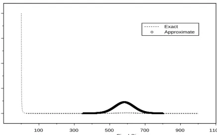
2.1 The final size distribution of an epidemic among a population of 800 individuals. . . 38 2.2 The final size distribution of an epidemic among a population of
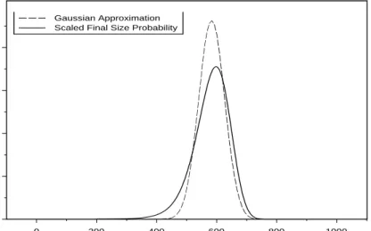
1000 individuals and the corresponding Gaussian approximation. 43 2.3 The scaled final size distribution of an epidemic among a
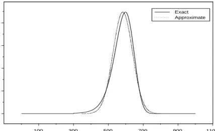
pop-ulation of 1000 individuals and the corresponding Gaussian ap-proximation. . . 45 2.4 The standardised final size probabilities of an epidemic among a
population of 1000 individuals and the corresponding Gaussian approximation. . . 47 2.5 Posterior density of R0 for the three different infectious periods
when x= 30. . . 51 2.6 Posterior density of R0 for the three different infectious periods
when x= 60. . . 53 2.7 Posterior density of R0 for the two different priors. . . 54
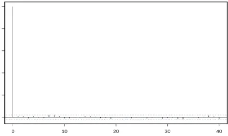
2.8 Plot of the autocorrelation function based on the posterior out-put of R0. . . 54
3.1 Posterior density of R∗ for two different priors. . . 73
3.2 Posterior trace plot of λL. . . 75
3.3 Plot of the autocorrelation function for λL. . . 75
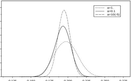
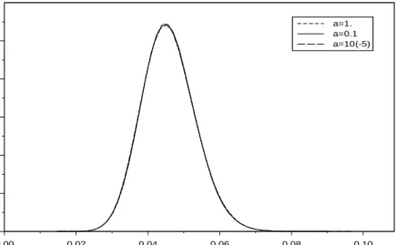
3.4 Posterior density of λG asα varies. . . 76
3.5 Posterior density of λL as α varies. . . 77
3.6 Posterior density of R∗ as α varies. . . 78
3.7 Scatterplot of λL and λG as α varies. . . 79
3.8 Graphical comparison of the likelihood for the three different methods. . . 96
4.1 The output for the total number of links for the smallpox dataset.132 4.2 The posterior density of λG for the two different priors. . . 133
4.3 The posterior autocorrelation function of λG. . . 135
4.4 Trace of the posterior density of λL from the Random Graph algorithm. . . 136
4.5 Trace of the posterior density of λG from the Random Graph algorithm. . . 137
4.6 Trace of the posterior density of the total number of local out-degrees. . . 138
4.7 Trace of the posterior density of the total number of global out-degrees. . . 139
4.8 The posterior density of λL from the Random Graph and the Severity algorithms. . . 140
4.9 The posterior density of R∗ from the Random Graph and the Severity algorithms. . . 141
4.10 Scatterplot ofλL and λG for the Tecumseh data when the infec-tious period follows a Gamma distribution. . . 142 4.11 The Posterior distribution of the mean local and global degree
for the Tecumseh data. . . 143 4.12 Posterior Density of λG for the two separate and the combined
Tecumseh outbreaks. . . 145 4.13 Posterior Density of λL for the two separate and the combined
Tecumseh outbreaks. . . 146 4.14 Posterior Density of R∗ for the two separate and the combined
Tecumseh outbreaks. . . 147 4.15 Posterior Density ofλGfor the two artificial datasets. We denote
with Data10 the dataset where all the values are multiplied by 10.148 4.16 Posterior Density ofλLfor the two artificial datasets. We denote
with Data10 the dataset where all the values are multiplied by 10.149 4.17 Posterior Density of R0 using the random graph algorithm and
the algorithm based on the multiple precision solution of the triangular equations. . . 153
List of Tables
2.1 Posterior summary statistics for the three different infectious periods when 30 out of 120 individuals are ultimately infected. . 50 2.2 Posterior summary statistics for the three different infectious
periods when 60 out of 120 individuals are ultimately infected. . 51 3.1 The Tecumseh influenza data . . . 73 3.2 Posterior parameter summaries from MCMC algorithm using the
Tecumseh dataset in the case that α = 1. . . 79 3.3 Posterior parameter summaries from MCMC algorithm using the
Tecumseh dataset in the case that α = 0.1. . . 80 3.4 Posterior parameter summaries from MCMC algorithm using the
Tecumseh dataset in the case that α = 10−5. . . . 82
3.5 The dataset of the first example . . . 83 3.6 Posterior parameter summaries for the data in Example 1. . . . 83 3.7 The dataset of the second example . . . 84 3.8 Posterior parameter summaries for the data in Example 2 using
the a Normal random walk proposal. . . 85 3.9 The ”perfect” dataset . . . 87 3.10 Posterior parameter summaries for the ”perfect” data. . . 88
3.11 The second simulated dataset . . . 88 3.12 Posterior parameter summaries for the second simulated dataset. 89 3.13 The third simulated dataset . . . 90 3.14 Posterior parameter summaries for the third simulated dataset. . 90 4.1 Posterior parameter summaries for the Influenza dataset with
households sizes truncated to 5 and with a Gamma distributed infectious period. . . 133 4.2 The 1977-1978 Tecumseh influenza data . . . 140 4.3 The 1980-1981 Tecumseh influenza data . . . 142 4.4 Posterior parameter summaries for the full 1977-1978 Influenza
dataset. . . 143 4.5 Posterior parameter summaries for the full 1980-1981 Influenza
dataset. . . 144 4.6 Posterior parameter summaries for the combined 1977-1978 and
1980-1981 Influenza datasets with household sizes up to 7. . . . 144 4.7 The Artificial dataset . . . 147 4.8 Posterior parameter summaries for the perfect data divided by 10
and rounded to the closest integer. The true values areλL= 0.06 and λG= 0.23. . . 151 4.9 Posterior parameter summaries for the smallpox data. . . 152
Chapter 1
Introduction to Stochastic
Epidemic Models, Bayesian
Statistics and Inference from
Outbreak Data
1.1
Introduction
In this thesis we will describe methods for Bayesian statistical inference for stochastic epidemic models. The focus will be on general methodology for the analysis of an epidemic model where the population is partitioned into groups. However, the approach can often be extended to more complex, and realistic population structures. The different methods are illustrated using both real life and simulated outbreak data.
This chapter serves as an introduction to the main themes that this thesis uses. Stochastic epidemic models are appropriate stochastic processes that can
be used to model disease propagation. Two processes of this kind are presented and their behaviour is outlined. Subsequently we give a brief introduction to Bayesian inference, which is the paradigm we shall follow throughout the thesis, and the modern computational tools used to facilitate the analysis of realisti-cally complex models. The last part of this chapter contains a short review of the analysis of infectious disease data using stochastic epidemic models.
1.1.1
Epidemic Modelling
Stochastic and Deterministic Models
We will focus on homogeneous and heterogeneous stochastic epidemic mod-els. Disease propagation is an inherently stochastic phenomenon and there is a number of reasons why one should use stochastic models to capture the transmission process. Real life epidemics, in the absence of intervention from outside, can either go extinct with a limited number of individuals getting ul-timately infected, or end up with a significant proportion of the population having contracted the disease in question. It is only stochastic, as opposed to deterministic, models that can capture this behaviour and the probability of each event taking place. Additionally, the use of stochastic epidemic models naturally facilitates estimation of important epidemiological parameters as will become apparent in the following chapters. Finally, from a subjective point of view, stochastic models are intuitively logical to define, since they naturally describe the contact processes between different individuals. However, the need for realistically complex models has made deterministic models more popular, since it is possible to analyse numerically quite elaborate deterministic models. Hence, it appears reasonable that effort should go towards developing general methods of statistical analysis that can be applied to complex stochastic
mod-els.
Modelling Disease Propagation
In recent years there has been increasing interest in the use of stochastic epi-demic models for the analysis of real life epiepi-demics. The need for accurate modelling of the epidemic process is vital, particularly because the financial consequences of infectious disease outbreaks are growing, two important recent examples being the 2001 foot and mouth disease (FMD) outbreak in the UK and the severe acute respiratory syndrome (SARS) epidemic in the spring of 2003. For modelling of these high impact epidemics see Ferguson et al. (2001) and Keeling et al. (2001) for FMD and Riley et al. (2003) and Lipsitch et al.
(2003) for SARS.
In order to prevent, or at least reduce, infection spread we need models that can accurately capture the main characteristics of the disease in question since understanding disease propagation is vital for the most effective reac-tive measures. Additionally, if we want to adopt a proacreac-tive approach and model vaccination strategies, we need methodology for performing statistical inference for the parameters of epidemiological interest. Hence, it readily be-comes apparent that it is vital that epidemic models of general applicability and methodology for their statistical analysis should be developed.
Two Stochastic Epidemics
In this chapter we will describe two stochastic epidemic models. The so-called generalised stochastic epidemic is a rather simple model defined on a homoge-neous and homogehomoge-neously mixing population. It is called generalised because the infectious period i.e., the time that an infective individual remains infec-tious, can have any specified distribution. The special case where the infectious
period follows an exponential distribution makes the model Markovian and is known as the general stochastic epidemic (e.g. Bailey (1975) chapter 6). Note that certain non exponential infectious periods (like Gamma with integer shape parameter) can be incorporated in a Markovian model using additional com-partments. However, the generalised stochastic epidemic is a unified process, even for infectious period distributions that cannot be written as the sum (or linear combination) of exponentials.
Subsequently, we describe a more complex model where the population is partitioned into groups and infectives have contacts both within and between the group. This model is motivated by a desire for additional realism since it is well known that disease spread is greatly facilitated in groups such as schools and households. The main reference for this so-called epidemic model with two levels of mixing is Ball et al. (1997). The generalised stochastic epidemic is a special case of the two-level-mixing model when all the households are of size one and we will evaluate our methods for this special case. Methods for statistical inference for epidemics will be reviewed in section four of this chapter. We shall now give a short introduction to Bayesian inference and the modern computational methods used for the implementation of the Bayesian paradigm.
1.1.2
Bayesian Inference
Introduction
Bayesian inference, similarly to likelihood inference requires a sampling model that produces the likelihood, the conditional distribution of the data given the model parameters. Additionally, the Bayesian approach will place a prior
combined using Bayes’ theorem to compute the posterior distribution. The posterior distribution is the conditional distribution of the unknown quantities given the observed data and is the object from which all Bayesian inference arises.
We shall now introduce some notation. The model parameters are described with the (potentially multi-dimensional) random variableθ. From the Bayesian
perspective, model parameters and data are indistinguishable, the only differ-ence being that we possess a realisation ofX, the observed data X =x. The frequentist and Bayesian approaches, despite arising from different principles do not necessarily give completely dissimilar answers. In fact, they can be con-nected in a decision-theoretic framework throughpreposterior evaluations (see Rubin, 1984). In this thesis we will adopt the Bayesian paradigm which, while theoretically simple and more intuitive than the frequentist approach, requires evaluation of complex integrals even in fairly elementary problems.
Modern Bayesian Statistics
The use of Bayesian methods in applied problems has exploded during the 1990s. The availability of fast computing machines was combined with a group of iterative simulation methods known as Markov chain Monte Carlo (MCMC) algorithms that greatly aided the use of realistically complex Bayesian models. The idea behind MCMC is to produce approximate samples from the posterior distribution of interest, by generating a Markov chain which has the posterior as its limiting distribution. This revolutionary approach to Monte Carlo was originated in the particle Physics literature in Metropoliset al. (1953). It was then generalised by Hastings (1970) to a more statistical setting. However, it was Gelfand and Smith (1990) that introduced MCMC methods to mainstream statistics and since then, the use of Bayesian methods for applied statistical
modelling has increased rapidly.
A comprehensive account of MCMC-related issues and the advances in statistical methodology generated by using this set of computational tools until 1995 is provided in Gilkset al. (1996). A contemporary similar attempt would be almost impossible since the use of MCMC has enabled the analysis of many complex models in the vast majority of the statistical application areas. In an introductory technical level, Congdon (2001) describes the analysis of a wide range of statistical models using BUGS, freely available software for Bayesian Inference using MCMC, see Spiegelhalteret al. (1996). Many of these models, including generalised linear mixed models, can only be approximately analysed using classical statistical methodology. Conversely, it is straightforward to analyse models of this complexity using routine examples of BUGS.
1.1.3
Inference from Outbreak Data using Epidemic
Mod-els
The Need for Epidemic Modelling
The statistical analysis of infectious disease data usually requires the develop-ment of problem-specific methodology. There is a number of reasons for this but the main features that distinguish outbreak data are the high dependence that is inherently present and the fact that we can never observe the entire infection process. In many cases the data from the incidence of an infectious disease consist of only the final numbers of infected individuals. Hence, the analysis should take into account all the possible ways that these individuals could be infected. Moreover, even when the data contain the times that the symptoms occur, we cannot observe the actual infection times. Also the true epidemic chain, i.e. who infects who, is typically not observed either.
These reasons suggest that in order to accurately analyse outbreak data, we need a model that describes a number of aspects of the underlying infection pathway. Hence, inference about the data generating process can provide us with an insight about the quantitative behaviour of the most important features of the disease propagation. Additionally, the design of control measures against a disease can be improved through a quantitative analysis based on an epidemic model.
The rest of the chapter is organised as follows. The two stochastic epidemic models and related results that we use throughout the thesis are presented in section 2. In section 3 we first give a short introduction to Bayesian theory while in the remainder of the section we present the main computational tools required for the implementation of the Bayesian paradigm. The chapter con-cludes with known statistical methodology for inference from infectious disease data.
1.2
Stochastic Epidemic models
1.2.1
Generalised Stochastic Epidemic model
Epidemic model
We describe a simple model for the transmission of infectious diseases where the population is assumed to be closed, homogeneous and homogeneously mixing. We define as closed a population that does not contain demographic changes. Hence, we assume that during the course of the epidemic no births or immigra-tions occur. We also assume homogeneity of the population in the sense that the individuals belong in the same group and each pair of individuals has the same degree of social contacts with each other. This assumption will be relaxed
later when we will assume that the population is partitioned into groups and individuals will have additional within-group contacts.
The population consists ofnindividuals out of whichmare initially infected and they are able to have close contacts i.e., contacts that result in infection, with other individuals of the population. The remainingn−m individuals are assumed to be initially susceptible and can be potentially infected by the m
initial infectives. The infectious periods of different infectives are assumed to be independent and identically distributed according to the distribution of a random variable I, which can have any arbitrary but specified distribution.
While infectious, an individual makes contacts with each of the n individ-uals of the population at times given by the points of a homogeneous Poisson process with intensity λn. The contacts result in immediate infection of the sus-ceptible individual that the infective has contacted. The infectious individual is removed from the infection process once its infectious period terminates. A removed individual can be dead, in case of a fatal disease, or recovered and immune to further infections. The Poisson processes of different individuals are assumed to be mutually independent. The epidemic ceases as soon as there are no infectives present in the population.
Epidemic models of this kind, where an individual is allowed to be in any of the three states, susceptible, infective or removed, are often called S-I-R epidemics. The special (Markovian) case where the infectious period follows an exponential distribution is known as the general stochastic epidemic. The assumption of an exponential infectious period is mathematically (and not bi-ologically) motivated since it makes the probabilistic and statistical analysis of the model simpler, see O’Neill and Becker (2002) and Streftaris and Gibson (2004) for applications on diseases with Gamma and Weibull distributed infec-tious periods respectively. The general stochastic epidemic was originated by
Bartlett (1949) and has received a lot of attention in the probabilistic litera-ture. However, it has been generalised in a large number of ways and we shall describe later in this section exact results for the case with a general infectious period.
Basic reproduction number
The most important parameter in epidemic theory is the basic reproduction number R0 (Dietz, 1993) defined as the expected number of infections
gener-ated by a “typical” infected individual in a large susceptible population. In the generalised stochastic epidemic a typical individual can be any of the in-fectives since the model is homogeneous and homogeneously mixing. In more complicated models the definition of a typical individual is not straightforward and care is required in the definition of an appropriate threshold parameter. We call R0 a threshold parameter since the value ofR0 determines whether or
not a “major” epidemic can occur. Specifically, whenR0 ≤1 the epidemic will
die out i.e., in an infinite population only a finite number of individuals will ultimately become infected. In the case that R0 >1 there is a positive
proba-bility that an infinitely large number of individuals will contract the disease in question.
The threshold theorem, described in the previous section, is the most im-portant result in the mathematical theory of epidemics and it was introduced in Whittle (1955), see also Williams (1971) and Ball (1983). We will present in the next section a rigorous derivation of the threshold parameter based on a coupling of the initial stages of the epidemic with a branching process. For the model presented here, R0 = λE[I]. We emphasize that the definition of
R0 as a threshold parameter and the related results are exactly valid only in
How-ever, this is the most commonly used epidemiological parameter to date and reducing R0 below unity is typically the aim of programs for epidemic control.
Final size distribution
We shall consider the case where only the final outcome of the epidemic is ob-served. Thefinal sizeof an epidemic is defined as the number of initially suscep-tible individuals that ultimately become infected. Letφ(θ) = E(exp(−θI)), θ >
0 be the moment generating function of the infectious periodI andpn
k the prob-ability that the final size of the epidemic is equal to k, 0 ≤ k ≤ n. Then Ball (1986) proved that l X k=0 n−k l−k pn k h φλ(nn−l)ik+m = n l , 0≤l≤n. (1.1)
The system of equations in (1.1) is triangular and thus, in principle, it is straightforward to calculate the final size probabilities recursively. However, numerical problems appear due to rounding errors even for moderate popula-tion sizes of order 50-100. Hence it readily becomes apparent that the calcu-lation of the likelihood, the distribution of the data given a parameter value, requires the development of a different method. In this thesis we will employ two ways to overcome these difficulties. In chapter two we will evaluate the likelihood using augmented precision arithmetic while in chapter four we shall use a random graph that enables the evaluation of the likelihood. We will now describe a more realistic, and complex, model for disease spread in a closed population.
1.2.2
Epidemic models with two levels of mixing
Basic modelIn this section we introduce the two-level-mixing model. The statistical analysis of this model will be described in later chapters. In this chapter we will define the model and give an approximation for the early stages of an epidemic in a population withlocal andglobal contacts. The relevant results that are required for inference purposes will be described in chapter three.
Population Structure We consider the model described in Ball et al.
(1997). The model is defined in a closed population that is partitioned into groups (e.g. households or farms) of varying sizes. Suppose that the popula-tion containsmj groups of sizej and let m =P∞j=1mj be the total number of groups. Then the total number of individuals isN =P∞
j=1jmj.
Epidemic Process We will make the S-I-R assumption so that each individ-ual can, at any timet≥0, be susceptible, infectious or removed. A susceptible individual j may become infectious as soon as he is contacted by an infec-tive and will remain so for a time Ij distributed according to any specified non-negative random variable I. The epidemic is initiated at time t = 0 by a (typically small) number of individuals while the rest of the population is initially susceptible. We allow individuals to mix at two levels. Thus, while in-fective, an individual makes population wide infectious contacts at times given by the points of a Poisson point process with rate λG. Each such contact is with an individual chosen uniformly at random from theN initially susceptible individuals. Hence, the person to person rate is λG
N . If the contacted individ-ual has been infected before then the contact has no effect to the state of this individual while if the contacted person is susceptible then he gets infective.
Additionally, each infective individual makes person to person contacts with any given susceptible in its own household according to a Poisson process with rateλL. All the Poisson processes (including the two processes associated with the same individual) and the random variablesIj, j = 1, . . . , N, describing the infectious periods of different individuals, are assumed to be mutually indepen-dent. Note here that bycontact we mean the so-called close contacts that result in the immediate infection of the susceptible. At the end of its infectious period the individual is removed and plays no further role in the epidemic spread. The epidemic ceases when there are no infectives present in the population.
Latent Period Note that this model does not assume a latent period for an infected individual. However, the distribution of the final outcome of an SIR epidemic is invariant to fairly general assumptions concerning a latent period, see Ballet al. (1997). One way to see this is to consider the infection process in terms of ”generations” of infectives. This is not always accurate for the propagation of a disease when temporal data about the epidemic spread are available, but there is no loss of generality when we consider final outcome data. This can be seen by considering the random graph associated with the epidemic and will become more clear when we will consider the construction of the random graph in chapter four. In what follows we describe some results regarding the coupling of the initial stages of the epidemic process with a suitable branching process.
Branching process approximation
The threshold parameter is of considerable practical importance since it gives information about epidemic control through prophylactic measures like vaccina-tion. For stochastic epidemic models threshold parameters are typically defined
as functions of the basic model parameters and the population structure. The probabilistic properties of the two-level-mixing model are analysed in Ball et al. (1997). The authors derive, among other limit theorems, a threshold result using a coupling argument. Specifically, assuming there is a population with infinitely many households, the initial stages of the epidemic are coupled with a branching process (see e.g. Jagers (1975)). The state-space of this branching process is the set of groups, with each group acting as a ”superindividual”. Thus, the early phase of the epidemic is coupled with a suitable stochastic process for which there is a large amount of theory available. Subsequently the authors prove, as the number of households goes to infinity, that during the early stages of the epidemic the probability of a global infectious contact with a member of an infected household is negligible.
Let us assume that for n = 1,2, . . ., the proportion mn
m of groups of size
n converges to θn as the population size N → ∞. Let also ˆg = P∞n=1nθn be the asymptotic mean group size and assume that ˆg <∞. Then it is shown in section 3.5 of Ballet al. (1997) that there exists, as the number of households goes to infinity, a threshold parameter defined by R∗ = λGE(I)ν. Here ν =
ν(λL) = 1gˆP∞n=1(1 +µn−1,1(1))nθn is the mean size of an outbreak in a group, started by a randomly chosen individual, in which only local infections are permitted and the initial infective in the group is included inν. Alsoµn−1,1(1)
is the mean final size of an epidemic in a group with a single initial infective and n−1 initial susceptibles where only local infections count. This quantity will be evaluated later using equation (3.4).
For simpler models this parameter would typically be the so-called basic reproduction number. However, for complex models it is not always straight-forward to define the basic reproduction number. Thus, we will be referring to
popu-lation, which in the current framework corresponds to all the households being of size 1, the threshold parameter would be R0 =λGE(I).
R∗is the threshold parameter that determines the behaviour of the coupled branching process. Hence, by standard branching process theory, ifR∗ ≤1 the branching process goes extinct, or equivalently, the epidemic will die out with probability 1. The epidemic extinction is defined in the asymptotic sense as mentioned in the previous section. Hence, in an infinite number of households, only a finite number of households will ultimately contain infected individuals. In the case of R∗ > 1 there is a positive probability that a major epidemic will occur. Thus, in a rigorous treatment of the non-extinction case, out of an infinite number of groups, a positive proportion of them will get infected from outside. The interpretation of the above results in terms of applications is that if one wants to prevent major epidemics using vaccination or other means of control, it will be necessary to keep R∗ below unity. Thus, it quickly becomes apparent that the estimation of the transmission parameters of the model is vital.
Approximating the initial stages of the epidemic is one of the two most important types of limit theorems in the epidemic theory. The second type describes results related to a normal approximation for the final size of an outbreak in the event of a major epidemic. Results of this kind for the two-level-mixing model will be described in chapter three, where a central limit theorem will be used for approximate statistical inference for this model.
This thesis utilises the Bayesian approach to statistical inference and in the next section we give a summary of the theory and the tools required for its implementation.
1.3
Bayesian Statistical Inference
1.3.1
Basic theory
In this section we will review the fundamentals of the Bayesian paradigm in a basic non-technical level. For a rigorous and detailed approach see Bernardo and Smith (1994).
Bayes’ Theorem
In the Bayesian approach, in addition to specifying the model for the observed data x = (x1, . . . , xn) given the vector of the unknown parameters θ, in the form of the likelihood function L(x| θ), we also define the prior distribution
π(θ). Inference concerning θ is then based on its posterior distribution, given
by
π(θ |x) = R L(x|θ)π(θ)
L(x|θ)π(θ)dθ ∝L(x|θ)π(θ). (1.2)
We refer to this formula as Bayes’ Theorem. The integral in the denominator is essentially a normalising constant and its calculation has traditionally been a severe obstacle in Bayesian computation. We shall demonstrate in the next section how we can avoid its calculation using MCMC methods. The second form in 1.2 can be thought of as “the posterior is proportional to the likelihood times the prior”. Clearly the likelihood may be multiplied by any constant (or any function ofxalone) without altering the posterior. Moreover, Bayes’ Theo-rem may also be used sequentially: suppose we have collected two independent data samples,x1 and x2. Then
π(θ |x1,x2)∝L(x1,x2 |θ)π(θ)
=L2(x2 |θ)L1(x1 |θ)π(θ)
∝L2(x2 |θ)π(θ |x1). (1.3)
That is, we can obtain the posterior for the full dataset (x1,x2) by first
eval-uating π(θ | x1) and then treating it as the prior for the second dataset x2.
Thus, we have a natural setting when the data arrive sequentially over time.
Prior distributions
In this section we briefly present the most popular approaches for the choice of a prior distribution. Additionally to the priors we mention here there exist the so called elicited priors, created using an expert’s opinion. However, elicitation methods go beyond the scope of this thesis and we shall not give more details here.
Conjugate priors When choosing a prior from a parametric family, some choices may be more computationally convenient than others. In particular, it can be possible to select a distribution which is conjugate to the likelihood, that is, one that leads to a posterior belonging to the same family as the prior. It is shown in Morris (1983) that exponential families, where likelihood functions often belong, do in fact have conjugate priors, so that this approach will typically be available in practice. The use of MCMC does not require the specification of conjugate priors. However, they can be computationally convenient and their use is recommended when it is possible and appropriate.
Non-informative priors In many practical situations no reliable prior in-formation concerningθexists, or inference based solely on the data is desirable.
In this case we typically wish to define a prior distributionπ(θ) that contains
no information about θ in the sense that it does not favour one θ value over
another. We may refer to a distribution of this kind as anoninformative prior
forθ and argue that the information contained in the posterior about θ stems
from the data only.
In the case that the parameter space is Θ={θ1, . . . , θn}, i.e., discrete and finite, then the distribution
π(θi) = 1
n, i= 1, . . . , n,
places the same prior probability to any candidateθvalue. Likewise, in the case of a bounded continuous parameter space, say Θ = [a, b],−∞ < a < b < ∞, then the uniform distribution
π(θ) = 1
b−a, a < θ < b,
appears to be noninformative.
For unbounded spaces the definition of noninformative distribution is not straightforward. In the case that Θ = (−∞,∞) a distribution like π(θ) = c
is clearly improper since R
π(θ)dθ = ∞. However, Bayesian inference is still possible in the special case whereR
L(x|θ)dθ =D <∞. Then
π(θ|x) = R L(x|θ)c
L(x|θ)cdθ =
L(x|θ)
D .
There is not however a “default” prior for all cases. The uniform prior is
not invariant under reparameterisation. Thus, an uninformative prior can be converted, in the case of a different model, to an informative one. One approach that overcomes this difficulty isJeffreys prior given by
where| · |denotes the determinant andI(θ) is the expected Fisher information
matrix, havingij-element
Iij(θ) = EX|Θ ∂2 ∂θi∂θj L(x|θ) .
In this thesis we will adopt the view of Box and Tiao (1973, p.23) who suggest that all that is important is that the data dominate whatever information is contained in the prior, since as long as this happens, the precise form of the prior is not important. Hence, we typically employ a few different priors with large variance and as long as the inference results do not change, then we shall consider our inference procedures as “objective”.
Inference Procedures
Having obtained the posterior distribution of interest we now have all the in-formation that the data contain for the parameters. A natural first step is to plot the density function to visualise the current state of our knowledge. Fur-thermore, we can obtain summaries of our posteriors which can give us all the information that can be obtained using a classical approach to inference plus, in certain cases, additional information. We will mention the most commonly used in practice, point estimation and interval estimation.
Point estimation Point estimation is readily available through π(θ | x).
The most frequently used location measures are the mean, the median and the mode of the posterior distribution since they all have appealing properties. In the case of a flat prior the mode is equal to the maximum likelihood estimate. For symmetric posterior densities the mean and the median are identical. More-over, for unimodal symmetric posteriors all the three measures coincide. For asymmetric posteriors the choice is not always straightforward. The median is often preferred since, in the case of one-tailed densities, the mode can be very
close to non-representative values while the mean can be heavily influenced in the presence of outliers. In practice, after visualising the posterior density, or a number of scatterplots in the case of multivariate densities, the evaluation of at least the mean and the median is recommended.
Interval estimation A 100×(1−α)% credibility set for θ is a subset C of
Θsuch that
1−α ≤P(C |x) = Z
C
π(θ |x)dθ,
where integration is replaced by summation for discrete components of θ. In
the case of continuous posteriors the ≤ is typically replaced by =.
This definition enables appealing statements like “The probability that θ
lies inC given the observed data xis at least (1−α)”. This comes in contrast with the usual interpretation of the confidence intervals based on the frequency of a repeated experiment. Probably the most attractive credibility set is the
highest posterior density, or HPD, set defined as
C ={θ ∈Θ:π(θ|x)≥ξ(α)},
where ξ(α) is the largest constant satisfying P(C | x) ≥ 1−α. A credibility set of this kind is appealing because it consists of the most likelyθvalues. In a
sampling based approach the calculation of the HPD set requires a numerical routine. Hence, it is easier to calculate the equal tail credibility set by simply taking theα/2- and (1−α/2)-quantiles ofπ(θ |x) which equals the HPD set
for symmetric unimodal densities.
There are a number of different approaches to Bayesian model assessment and model choice. We will not consider these issues here since they extend beyond the scope of this thesis. For a discussion of several key ideas in the field, including Bayes factors and model averaging, see Berger (1985). We will now
consider a collection of algorithms that greatly facilitate the implementation of Bayesian modelling known as Markov chain Monte Carlo (MCMC) algorithms.
1.3.2
Bayesian Computation
The main idea behind MCMC is to generate a Markov chain which has as its unique limiting distribution the posterior distribution of interest. It dates back to the seminal paper of Metropolis et al. (1953) although the computational power required was not available at the time. The original generation mecha-nism was generalised by Hastings (1970) in theMetropolis-Hastings algorithm
that we shall describe in the following section.
The Metropolis-Hastings algorithm
The objective of the Metropolis-Hastings (M-H) algorithm is to generate ap-proximate samples from a density π(θ) known up to a normalising constant. Given a conditional density q(θ′ | θ) the algorithm generates a Markov chain (θn) through the following steps:
1. Start with an arbitrary initial valueθ0
2. Update fromθn toθn+1 (n= 0,1, . . .) by (a) Generateξ ∼q(ξ |θn) (b) Evaluate α=minnπ(ξ)q(θn|ξ) π(θn)q(ξ|θn),1 o (c) Set θn+1 = ξ with probability α, θn otherwise.
The distribution π(θ) is often called the target distribution whereas the dis-tribution with density q(· | θ) is the proposal distribution. The algorithm
described above will have the correct stationary distribution as long as the chain produced is irreducible and aperiodic. This holds true for an enormous class of proposals and usually it suffices, but is not necessary, that the support of the proposal distributionq(· |θ) contains the support ofπ for everyθ. How-ever, the generality of the theorem suggests that the selection of the proposal can be rather decisive. In practice, a proposal with poor overlap between the high density region of π and q(· | θ) may considerably slow convergence. We will now describe the most popular proposal distributions.
The Independent Case A proposal distribution is called independent if it does not depend on θ. This family of distributions admits the form
q(θ′ |θ) =f(θ′).
This class of proposals can in theory result in algorithms with satisfactory properties as described in Mengersen and Tweedie (1996). In practice the choice of the actual proposal can affect the mixing of the Markov chain drastically. A proposal that is badly calibrated, i.e., a distribution with little support over the high density region of the target distribution, can have extremely slow mixing. Ideally the proposal should resemble the target density being somewhat more diffuse. Usually MCMC algorithms are not based on an independence sampler alone but make use of a number of proposals. However, it is worth emphasizing that a well calibrated independence sampler can outperform most M-H algorithms. We will now describe the most common choice for q(· | θ), the symmetricrandom walk proposal.
Random Walk Metropolis The natural idea behind the random walk pro-posal is to perturb the current value of the chain at random and then check whether the proposed value is likely for the distribution of interest. In this
case the proposal has the form q(θ′ |θ) =f(kθ′ −θk) where k · k denotes the absolute value. Thus, the proposed value in the M-H algorithm is of the form
ξ =θn+ǫ,
where ǫ is distributed according to a symmetric random variable. For this random walk proposal the acceptance ratio becomes
α =min π(ξ) π(θn) ,1 .
Hence, the chain will remain longer in points with high posterior value while points with low posterior probability will be visited less often. The most popu-lar choices for the proposalq(· |θ) are the normal, the uniform and the Cauchy distributions. In fact, the Gaussian random walk has been, along with the Gibbs sampler described in the next paragraph, among the most commonly used MCMC schemes to date. The algorithm is widely applicable and the only requirement is the scaling of the variance of the proposal. For the Gaussian case Roberts et al. (1997) proved that the optimal scaling of the proposal should result to an acceptance rate of approximately 0.234, at least for high-dimensional situations. We will now turn our attention to the Gibbs sampler, the most popular MCMC method, particularly in the years following the paper of Gelfand and Smith (1990).
The Gibbs Sampler The Gibbs sampling approach is a special case of the M-H algorithm directly connected to the target distribution π. The method derives its name from Gibbs random fields, where it was used for the first time by Geman and Geman (1984). The idea is to sample from the joint posterior distribution π(θ1, θ2, . . . , θℓ) using the one-dimensional full conditional distri-butionsπ1, π2, . . . , πℓ. Thus, given the current state of the chain θn1, θ2n, . . . , θℓn we simulate the next state of the chain by sampling
The Gibbs sampler has acceptance probability one. Hence, each sample is a successive realisation from the chain. Theθi’s and the full conditional distribu-tions need not be one-dimensional. In fact, for correlated parameters,blocking
can improve the convergence of the chain considerably. Moreover, when sim-ulation from a given conditional distribution πi(θi | θj, j 6= i) is complicated, possibly due to the absence of a closed-form distributional formula, this simu-lation can be replaced with a Metropolis-Hastings step havingπi(θi |θj, j 6=i) as the target distribution. Also sampling from the full conditional distribu-tions is not necessarily done in a systematic way. The random scan Gibbs sampler, choosing which full conditional distribution to update at random, can have superior convergence properties in certain cases. These are only the most basic variants of the Metropolis-Hastings algorithm. A vast number of modifi-cations and combinations, leading tohybrid samplers, appear in the literature. However, these methods go beyond the scope of this chapter and we shall not pursue these issues further.
Implementation
MCMC methods have generated unlimited applicability of the Bayesian paradigm in nearly every branch of statistics. However, the user should always be cau-tious since the method is based on asymptotic arguments. Hence, there are two practical issues that need investigation to establish the reliability of the chain outcome. The first of these is the burn in, i.e. the number of iterations that need to be discarded from the output.
Burn In The Markov chains produced with the proposal distributions that we described thus far are ergodic. This means that the distribution of (θn) converges, asngoes to infinity, toπ(· |x) for every starting value (θ0). However,
the speed of this event i.e., the rate of convergence varies depending, among others, on the posterior state-space and the sampler used, see Roberts (1996) for a discussion of these issues. Thus, for k large enough, the resulting (θk) is an approximate sample fromπ(θ|x). The problem in practice is to determine what a “large”k means. There is a number of diagnostic tests proposed in the literature that provide us with different indicators on the stationarity of the chain. However, none of these tests can actuallyguaranteeconvergence. Hence, throughout this thesis we investigate the “trace”, a plot of the history, of the chain for very long (typically a few million iterations) runs and all the results reported in this thesis are based on chains that appear to have converged. The second practical concern is that after the burn-in some thinning of the chain may be required.
Thinning The sample we obtain, after the initial observations are discarded, doesnot necessarily consist of independent observations. In theory this is not crucial if we are interested in functionals of π(θ | x) since the Ergodic Theo-rem implies that the average L1 PL
ℓ=1f(θℓ) converges, as L goes to infinity, to
Eπ(f(θ)). In practice however, some sort of batching may be required. Hence, keeping one sample of the chain out of t iterations, with t = 20 ort = 50 say, we can achieve approximate independent sampling from π(θ | x). Moreover, from the practical point of view, we avoid the creation of unmanageable sample sizes that could potentially hamper the statistical analysis of the output.
1.4
Statistical Inference from Outbreak Data
1.4.1
The Nature of Infectious Disease Data
The Reasons for Modelling
The statistical analysis of infectious disease data is typically not a straight-forward problem and as such it requires the development of problem specific methodology. Infectious disease data are usually complicated to analyse and there are a number of reasons that makes their analysis awkward. We shall describe the features of infectious disease data in the following section.
The analysis of outbreak data can be more effective when based on a model for the actual mechanism that generates the data. Moreover, epidemic models provide us with a better understanding of the infection process and also with the epidemiologically important quantities of interest. Finally, there are a number of reasons for the analysis, using epidemic models, of historical incidence data. Analyses of this kind can be very useful for diseases occurring due to both novel and re-emerging pathogens as described in the recent review of Fergusonet al.
(2003). This is of particular relevance at the moment, not only because of the emergence of the SARS outbreak, e.g., Riley et al. (2003) and Lipsitch et al.
(2003), but also due to the threat of deliberately released pathogens such as smallpox, e.g. Kaplanet al. (2002) and Halloran et al. (2002). Fergusonet al.
(2003) argue that there does not exist an epidemic model that can be “truly predictive” in the context of smallpox outbreak planning and consequently that no control method can be a priori identified as absolutely optimal. However, they suggest that it is vital that a range of models and a set of control options can be identified. Hence, in the event of an outbreak, the models can be adjusted in order to identify the current optimal control method. We shall now describe in detail the difficulties arising during the statistical analysis of
infectious disease data.
The Features of Infectious Disease Data
One of the complications when analysing infectious disease data is that there are often various levels of inherent dependence that one needs to take into ac-count, particularly in the event of a “major” epidemic. Specifically, despite the fact that stochastic epidemics are typically easy to define, there is often a very large number of ways that can result to the same outcome. The complexity of the models increases enormously as they become more realistic. Hence, as-suming biologically plausible distributions for the infectious periods, such as Gamma and Weibull instead of the mathematically convenient constant and ex-ponentially distributed ones, induces an additional level of dependence. These facts come in contrast with the usual independence assumption that under-lies many of the standard statistical methods. Moreover, the actual disease incidence data are incomplete in different ways. In particular, a relatively in-formative dataset consists of the times at which the infectious individuals are detected. Even this level of information however is far from being complete. From the inference viewpoint it would be desirable to observe the times that the individuals did contract the disease, as well as the time that the individuals ended their (potential) latent period and could infect others. Additionally, a significant number of data sets only consist of the numbers of individuals who contracted the disease in question. These data can be important data, verified by clinical measurements, or routinely collected surveillance data. However, when realistically complex models are to be fitted to data of this kind, the likelihood can be analytically and numerically intractable. We shall explore in this thesis a number of imputation methods, i.e., different ways of adding information about the epidemic process, that can aid towards overcoming these
difficulties.
It is this nature of epidemic data that makes the statistical analysis of in-fectious disease data particularly challenging. In the remainder of this section we shall review the work conducted thus far on statistical inference, Bayesian and classical, from outbreak data and we will complete the section with infer-ence about the epidemic models related to the stochastic epidemic model with two levels of mixing that will be the subject of statistical inference in chapters 3 and 4.
1.4.2
Previous Work on Epidemic Modelling
Monographs on Epidemic Models
There is a vast literature on deterministic and stochastic epidemic modelling. We shall mention here the main books on epidemic modelling. Most of the work on modelling disease transmission prior to 1975 is contained in Bailey (1975). The author presents a comprehensive account of both stochastic and deterministic models, illustrates the use of a variety of the models using real outbreak data and provides us with a complete bibliography of the area.
Becker (1989) presents statistical analysis of infectious disease data. The author uses a number of different models and analyses a large variety of real life outbreak data. The single book that has received most attention recently is Anderson and May (1991). However, the authors only focus on deterministic models, as does the recent monograph by Diekmann and Heesterbeek (2000). A six-month epidemics workshop took place in 1993 in the Isaac Newton Institute in Cambridge. A large part of the outcome of the work conducted in this meet-ing is summarised in the three volumes edited by Grenfell and Dobson (1996), Isham and Medley (1996) and Mollison (1996) respectively. A recent addition
to the literature of stochastic epidemic modelling is Andersson and Britton (2000) which provides an excellent introduction to stochastic modelling and the authors also mention some basic statistical analysis for stochastic epidemic models. Since the seminal paper of Mollison (1977) on spatial epidemics there has been increasing interest in the applied probability literature for models of this kind. Also, a number of spatial epidemic models based on bond-percolation has been developed since the paper of Kulasmaa (1982), see for example the book by Liggett (1999) and the references therein.
Reviews of Epidemic Models and their Analysis
There does not exist a monograph concerned with the recent progress on the statistical analysis of infectious disease data. Becker and Britton (1999) present a critical review of statistical methodology for the analysis of outbreak data. The authors make an attempt to place emphasis on the important objectives that analyses of this kind should address, as well as suggesting issues where further work is required. Recently, Ferguson et al. (2003) conducted a review of epidemic models with reference to planning for smallpox outbreaks. The authors emphasize the importance of epidemic modelling as a useful tool for assessing the threat posed by deliberate release of a known pathogen, as well as dealing with the emergence of a novel virus. We shall now present the statistical analysis of epidemics that are relevant to the models that this thesis will attempt to explore.
Statistical Analysis of Epidemic Models
This section will review methods of parametric inference about the infection rate(s) and the epidemiologically important parameters. See Becker (1989) for a comprehensive account of nonparametric inference methodology based on
martingale methods.
Epidemics in homogeneous populations The first statistical analysis of removal data, based on a continuous-time model, for the purpose of estimating the infection and the removal rate is described in Bailey and Thomas (1971). The authors analysed the general stochastic epidemic using maximum likeli-hood methods. Rida (1991) derives asymptotic normality results for some esti-mators of the infection rate and the corresponding basic reproduction number. However, the largest amount of information for inference based on epidemic models defined on a homogeneous population is in Becker (1989). A large number of different approaches are presented including the author’s work for parametric as well as non-parametric methods of statistical inference.
As with many application areas of statistics, inference for stochastic epi-demic models has benefited considerably from the use of Markov chain Monte Carlo methods. In particular, Gibson and Renshaw (1998) and O’Neill and Roberts (1999) first presented a statistical analysis of S-I-R models based on MCMC methods. O’Neill and Becker (2001) have presented inference proce-dures for a non-Markovian epidemic model where the infectious period follows a Gamma distribution. Streftaris and Gibson (2003) use MCMC methods in a different extension of the general stochastic epidemic model where the infectious period is distributed according to a Weibull random variable, with particular reference to plant epidemiology. Finally, Hawakaya et al. (2003) extend the basic model in two key directions. They allow for a multitype (e.g. different age, sex) model, where the infection rates vary between different types, as well as the actual number of susceptibles being unobserved. The authors derive statistical inference for both the infection rates and the size of the population. We shall briefly mention three papers that focus more on the statistical
context of inference for epidemics, as opposed to inference for a wider class of epidemic models than those analysed before. A group of parameterisations that can improve the convergence of MCMC algorithms used in the epidemics context is the subject of Neal et al. (2003). Specifically, the authors describe algorithms that can be more robust with respect to the mixing of the Markov chain. A method that eliminated the need for assessing convergence of the Markov chain is the perfect simulation algorithm originated by Propp and Wilson (1996). O’Neill (2003) proposes methods of perfect simulation when the infection process is of the Reed-Frost type. Finally, a different statistical method, based on the forward-backward algorithm, that can be used for esti-mation of the infection and removal rate in the general stochastic epidemic is presented in Fearnhead and Meligkotsidou (2003). Statistical inference is less obvious when the population in question admits a particular structure, e.g. households, and these methods will be described in the next paragraph.
Epidemics in structured populations
Epidemics on independent households Longini and Koopman (1982) consider models in which individuals reside in households and may be poten-tially infected both from infectives within their household or from individuals outside their household. Their model assumes that the disease within the household progresses independently of the dynamics of the community. This approach is generalised in a model with a general infectious period in Addy
et al. (1991). The authors extend the work of Ball (1986) on the generalised stochastic epidemic so that individuals can also be infected from the community at large. We will comment further on the approach of Addy et al. (1991) and the limitations of their model in chapters 3 and 4. Britton and Becker (2000) use the Longini-Koopman model in order to estimate the critical vaccination
coverage required to prevent epidemics in a population that is partitioned into households. O’Neill et al. (2000) use MCMC method to analyse both tem-poral and final size data from household outbreaks. Finally, a different perfect simulation method is applied in Clancy and O’Neill (2002) where the authors analyse a model related to the Longini-Koopman model where some variation in the probability of individuals from different households being infected from outside is included.
Probably the most important application of epidemic models is in epidemics control, typically using vaccination. A large body of literature exists and we shall only mention a few key references. Becker and Dietz (1995) study the control of diseases among households assuming that once there is an infective in a household everybody contracts the disease. Ball and Lyne (2002) derive the effect of different vaccination policies in a population that is partitioned into households while Becker et al. (2003) use an independent households model to estimate vaccine efficacy from household outbreak data, see Halloran
et al. (1999) for a review of other methods for estimating vaccine efficacy. We shall now mention briefly statistical inference for epidemics with two levels of mixing.
Inference for Epidemics with two levels of mixing Ball et al.
(1997) briefly consider statistical inference for their model. They mention that, for estimation purposes, their model can asymptotically be approximated by the model of Addy et al. (1991). The authors use the basic idea and the results from Addy et al. (1991) to examine different vaccination strategies among households. Britton and Becker (2000) also formulate their work in order to estimate the immunity coverage required for preventing an outbreak when the population is partitioned into households, in terms of the two-level-mixing model. However, as mentioned in the previous paragraph, they perform
their statistical inference with respect to an independent households model. A more detailed approach that utilises (pseudo)likelihood inference is presented in Ball and Lyne (2003). The authors describe inference procedures for the multitype version of the model described in Ball and Lyne (2001). The method used is related to the method we describe in chapter 3 and we will comment on specific results in the appropriate sections of chapter 3.
Epidemics with different population structure In real life popula-tions individuals interact with a number of different environments additionally to their household, such as schools and workplaces. However, it would be im-possible to capture every aspect of the population structure. In the recent years there has been intense activity in describing the population structure through a random network structure. Probably the simplest model of this kind is a Bernoulli random graph where each individuals has social contacts with other individuals in the populations according to a fixed probability. Britton and O’Neill (2002) use MCMC methods to conduct Bayesian Inference for a model where individuals have social contacts according to a Bernoulli random graph and the disease spreads as a general stochastic epidemic. Neal et al. (2003) extend their reparameterisations in this case to offer robust MCMC algorithms for the infection and removal rate as well as the probability of social contact.
These methods can, in principle, be extended to more complicated social structures. It would be particularly interesting to consider statistical inference when the population is assumed to have social contacts according to a complex random graph. There has been intense recent interest in sociology and sta-tistical mechanics since the pioneering work of Watts and Strogatz (1998) on “small-world” networks, see for example the review by Strogatz (2001). Albert and Barab`asi (2002) present an extensive review of the different models for the structure of the community and other networks such as the internet and
vari-ous biological networks, including the so-called scale free networks. A number of algorithms have been developed for the detection of these structures and it would be interesting to combine our approach with an approach of the kind de-scribed in Newman (2003). Finally, there has been some interest in statistical inference for spatio-temporal epidemic models, see for example Gibson (1997) and Marion et al. (2003).
Chapter 2
Exact Results for the
Generalised Stochastic Epidemic
2.1
Introduction
This chapter contains methods for the numerical solution of the set of the triangular equations describing the final size probabilities of the generalised stochastic epidemic. This simple stochastic process was described in the previ-ous chapter, although no attempt was made to describe statistical analysis of the model. The probabilities of the final size can be derived from a well known set of recursive equations, see Ball (1986). However, practical implementation of attempts to solve these equations is frequently hampered b