DOI 10.1007/s10182-011-0152-7 O R I G I N A L PA P E R
Statistical concepts of a priori and a posteriori risk
classification in insurance
Katrien Antonio·Emiliano A. Valdez
Received: 24 September 2010 / Accepted: 9 January 2011 / Published online: 2 February 2011 © The Author(s) 2011. This article is published with open access at Springerlink.com
Abstract Everyday we face all kinds of risks, and insurance is in the business of
providing us a means to transfer or share these risks, usually to eliminate or reduce the resulting financial burden, in exchange for a predetermined price or tariff. Ac-tuaries are considered professional experts in the economic assessment of uncertain events, and equipped with many statistical tools for analytics, they help formulate a fair and reasonable tariff associated with these risks. An important part of the process of establishing fair insurance tariffs is risk classification, which involves the grouping of risks into various classes that share a homogeneous set of characteristics allowing the actuary to reasonably price discriminate. This article is a survey paper on the sta-tistical tools for risk classification used in insurance. Because of recent availability of more complex data in the industry together with the technology to analyze these data, we additionally discuss modern techniques that have recently emerged in the statistics discipline and can be used for risk classification. While several of the il-lustrations discussed in the paper focus on general, or non-life, insurance, several of the principles we examine can be similarly applied to life insurance. Furthermore, we also distinguish between a priori and a posteriori ratemaking. The former is a process which forms the basis for ratemaking when a policyholder is new and in-sufficient information may be available. The latter process uses additional historical
Katrien Antonio acknowledges financial support from NWO through a Veni 2009 grant. K. Antonio (
)University of Amsterdam, Roetersstraat 11, 1018 WB Amsterdam, The Netherlands e-mail:[email protected]
K. Antonio
Katholieke Universiteit Leuven, Naamsestraat 69, 3000 Leuven, Belgium E.A. Valdez
Department of Mathematics, University of Connecticut, 196 Auditorium Road, Storrs, CT 06269-3009, USA
information about policyholder claims when this becomes available. In effect, the re-sulting a posteriori premium allows one to correct and adjust the previous a priori premium making the price discrimination even more fair and reasonable.
Keywords Actuarial science·Regression and credibility models·Bonus–Malus systems
1 Introduction
Facing risks, or unexpected events, is part of our everyday life. A wide range of sit-uations can be enumerated to illustrate this statement. Rain on your wedding day, a traffic jam when you are already late for an appointment or a black fly in your Chardonnay are examples of pernicious scenarios that simply cause some annoying irritation, but which may also be classified as risks. On the other hand, risks result-ing into more tragic disaster such as a fire, an accident or unemployment, illustrate examples that can have a huge impact on one’s economic and personal situation.
Many of us are aware of these risks we face everyday, especially those with pos-sible huge economic impact. There is some level of risk aversion in all of us in the sense that to avoid being affected when these risks occur, we look for possible ways to transfer some or all of these risks to other economic agents in the market willing to assume them. In light of this risk aversion brought the birth of a whole sector of activities that we find today willing to provide us the needed protection: the business of insurance. Risk compensation by grouping similar, independent risks forms the basis of actuarial practice: “The contributions of the many to the misfortunes of the few” as the motto of Lloyd’s of London says.
The discipline of actuarial science deals with uncertain events where clearly the concepts of probability and statistics provide for an indispensable instrument in the measurement and management of risks. An important aspect of the business of insur-ance is the determination of the price, typically called premium but preferably called tariff in this paper, to pay in exchange for the transfer of risks; it is the job of the ac-tuary to evaluate a fair price given the nature of the risk. In this article, we provide for a survey and discussion of contemporary statistical techniques that can be practically implemented for pricing risks through ratemaking based on risk classification. 1.1 Ratemaking and risk classification
Clearly then within the actuarial profession, a major challenge can be found in the measurement and construction of a fair tariff structure. This is the objective of a ratemaking process. Pricing risks based upon certain specific characteristics has a long history in actuarial science, e.g. McClenahan (2001) observed that 18th century fire insurance rates for dwellings in the United States were based upon roof type and basic construction. Premium rates for marine insurance, believed to be the oldest form of insurance, are based on characteristics of the design and built-in protection of each ship and several ships vary in design.
Indeed, in light of the heterogeneity within an insurance portfolio, an insurance company should not apply the same premium for all insured risks in the portfolio.
Otherwise the so-called concept of adverse selection could undermine the solvency of the company and possibly lead to the collapse of the insurance market. On one hand, ‘good’ risks, with low risk profiles, could pay too much and eventually, prefer to leave the company. On the other hand, ‘bad’ risks may find a uniform tariff to be in their favor and therefore, prefer to stay with the company. This could lead to a spiral effect where the insurer could end up with a disproportionate number of ‘bad’ risks in its portfolio and to remain solvent, it may have to keep increasing its premium rates. Therefore, it is important for the insurer to optimally group the risks in the portfo-lio so that those insureds with similar risk profile pay the same reasonable premium rate. Such is the idea behind risk classification within the ratemaking process. A risk classification system should not only allow insurers to price discriminate their prod-ucts in a fair and equitable manner, but should also be constructed based on a sound statistical basis.
To construct a tariff structure that reflects the various risk profiles in a portfolio within a reasonable and statistically sound basis, actuaries usually rely on regres-sion techniques. Such techniques allow for the incluregres-sion of various explanatory (also called classifying or rating) variables so that the actuary is able to construct risk classes with more or less similar risk profiles. For non-life (also called: property and casualty or general) insurance, typical response variables in these regression models are the number of claims (or claim frequency) per unit of exposure on the one hand, and the corresponding amount of loss, given a claim (or claim severity) on the other hand. A formal discussion of these actuarial terminologies will follow in Sect.2.1. That section also explains how regression models for claims frequency and severity allow us to estimate the price of risk.
Different classifying variables impacting either frequency or severity (or both) can be found in all forms of insurance. For example, in automobile insurance, a non-life product, it is typical to find the following classifying variables used: age-gender-marital status, use of the car, geography (location of garage) and other factors such as whether the vehicle is a sports car or not. The cost of claims may be influenced among others by factors such as the use of the car (more driving implies more exposure to claims, driving conditions: time of day, weather, area), driving ability (experience and training, reaction time, eyesight and hearing, condition of the car, driving style), interaction with the claims mechanism and the extent of damages (crashworthiness of the car where certain brands are able to withstand severity of accidents better than others, use of safety devices). See Finger (2001) for further discussion. In fire insur-ance, studies have shown that restaurants have a higher frequency of accidents than stores; the presence of a sprinkler system, the value of the building and contents be-ing insured all can impact the amount of damage in the event of a fire. For workers’ compensation, a form of insurance that provides protection for injuries in the course of employment, statistics show significant difference in claims for various sectors of employment, e.g. manufacturing versus education, with employees in manufacturing firms indicating larger claims frequencies. While several characteristics may impact both frequency and severity, some affect severity but not frequency, and vice versa. To illustrate, the presence of a sprinkler system may not affect the frequency of claims but clearly affects the severity. Finally, risk classification systems are also found in life insurance. During the underwriting process for the purchase of life insurance, the
insurer collects information on the applicant’s risk factors (e.g. age, gender, smoking habits, occupation, any dangerous hobbies, and personal and family health history) through a questionnaire and possibly, a medical examination. The information is then used to classify policyholders into risk classes and to price their policies accordingly. See Dickson et al. (2009) for a discussion. However, risk classification for life insur-ance products is beyond the scope of this article.
In the construction of a risk classification system, the statistical considerations, often referred to as the actuarial criteria, are but one of several, but of utmost impor-tance, criteria for selecting classifying or rating variables. This survey paper focuses on these criteria. Here, we ensure that the classifying variable must be considered to: (1) be accurate in the sense that it has a direct impact on costs, (2) meet homo-geneity requirement in the sense that the resulting expected costs within a class are reasonably similar, (3) be statistically credible and reliable. Other considerations for the selection of variables are practical or operational implementation, “social accept-ability”, and legal considerations. To illustrate for example, the use of “gender”, even if statistically sound, as a classifying variable may be restricted for certain forms of insurance because sex discrimination is prohibited according to some constitutions. For further discussion of these criteria, we refer the reader to Finger (2001).
1.2 A priori and a posteriori ratemaking
When the explanatory variables used as rating factors express a priori correctly mea-surable information about the policyholder (or, for instance, the vehicle or the insured building), the system is said to be an a priori classification scheme. A discussion of a priori rating will follow in Sect.2. However, an a priori system is unable to identify all the possible important factors because some of them are either unmeasurable or unobservable. Take the case for example of automobile insurance where the insurer is unable to detect the driver’s aggressiveness behind the wheel or the quickness of his reflexes to avoid a possible accident. Thus, tariff cells within an a priori rating system will never be completely homogeneous. For that reason, an a posteriori or an experience rating system is necessary to allow for the re-evaluation of the premium by taking into account the history of claims of the insured as it becomes available. The statistical philosophy behind this is that the best (or optimal in some sense) pre-dictor for the future number of claims that an insured will report is conditionally based on the number of claims reported in the past. The actuarial credibility systems discussed in Sects.3.1and3.2are examples of a posteriori rating systems that take into account the history of claims as it emerges for an individual risk. Commercial versions of these experience rating schemes are more widely known in practice as Bonus–Malus scales. Rating schemes according to these Bonus–Malus scales is the topic of Sect.3.3.
1.3 Statistical techniques for risk classification
Since the early development of constructing a priori and a posteriori rating schemes, ordinary regression techniques based on the assumption of Normal data has been the standard norm in practice. See, for example, Lemaire (1985). Several papers based
on this technique have appeared in the actuarial literature, but actuaries have real-ized that insurance data usually violate the assumption of the Normal distribution. Recent advances in statistical modeling, spurred both by the availability of more data and computing technologies to analyze these data, have emerged. The applications of these up-to-date statistical techniques in the analysis of insurance data have pro-vided avenues for further developing skills for actuarial modeling. This article high-lights some of these advances in the literature and those that are slowly crawling up in practice. Within the context of a priori ratemaking, for example, it is becoming a standard norm in practice to use Generalized Linear Models (GLMs) where data is modeled within the class of exponential dispersion distributions. Other advances, which include Generalized Additive Models (GAMs), regression models based on generalized count distributions and heavy-tailed regression models for claims sever-ity, can be used in the context of a priori ratemaking. These topics are discussed in Sect.2.
In Sect.3, we emphasize our discussion on risk classification and a posteriori ratemaking. Several of the statistical models discussed in this section cover topics that are lesser known in practice, for example, models for clustered data (panel data and multilevel data) are discussed. In addition, we also consider the two types of model estimation: likelihood-based and Bayesian estimation methods. The latter method has the advantage of allowing the analyst to construct a full predictive distribution of quantities of interest. In our discussion of Bonus–Malus schemes, some concepts of Markov chains necessarily appear because of the possible transition through the various Bonus–Malus scales.
We present numerous examples based on real-life actuarial data throughout the paper to illustrate several of the methodologies. These illustrations can help practi-tioners implement these techniques in practice. Denuit et al. (2007) provides for an excellent and comprehensive reference on several aspects of a priori and a posteriori risk classification, with an emphasis on claim frequency. Frees (2010) is a useful ref-erence that contains several case-studies to illustrate statistical regression models for insurance rating.
2 Regression models for a priori risk classification
Regression techniques are indispensable tools for the pricing actuary. Here in this section, we focus on two types of response variables that are important in pricing for short term insurance contracts: the number of claims (or claim frequency) per unit of exposure and the amount of claim given a claim occurs (or claim severity). In Sect.2.1definitions follow of actuarial concepts relevant in ratemaking (e.g. expo-sure, frequency and severity). It is also explained how risk classification models for both frequency and severity are combined to calculate a so-called pure premium. Sec-tion2.2presents current industry practice for risk classification based on generalized linear models. More advanced statistical methods are illustrated in Sect.2.3. 2.1 Frequency, severity and pure premium for cross-sectional data
Some actuarial concepts, crucial for ratemaking, are discussed below. See McClena-han (2001) and Frees (2010) for further details. The basic rating unit underlying an
insurance premium is called a unit of exposure. In our examples from automobile in-surance, earned exposure is used and this refers to the fraction of the year for which premium is paid and therefore coverage is provided. Another example is workers compensation where company payroll is typically used as exposure base. When an insured demands for a payment under the terms and conditions of an insurance con-tract, this is referred to as a claim. Claim frequency refers to the number of times a claim is made during a (calendar) year and is expressed in terms of frequency per ex-posure unit. The amounts paid to a claimant under the terms of an insurance contract are called losses and severity is the term used for the amount of loss per claim.
Insurers typically keep track of frequency and severity data in separate files. In the policyholder file, underwriting information is registered about the insured (e.g. age, gender, policy information such as coverage, deductibles and limitations) and additional information may be kept about the claims event. In the claims file, infor-mation is recorded about the claims filed to the insurer together with the amounts and payments made. With a priori rating each individual risk is priced based on the history of frequency and severity observed usually from a cross-sectional data set. Cross-sectional means that the data base contains information fromNpolicyholders, but the time series structure of the data is ignored.
Typically from these files, we find that for each insuredithe observable responses are:
• Ni: the number of claims and the total period of exposureEi during which these
claims were observed; and
• Cij the loss corresponding to each claim made (withj=1, . . . , Ni).
The set{Cij}is empty whenNi =0. The so-called aggregate lossLi is defined as
Li:=Ci1+ · · · +CiNiand refers to the total amount of claims paid during the period
of observation. The data available then to the insurer for a priori rating typically have one of the following formats:
(1) {Ni, Ei, Ci1, . . . , CiNi}, thus the vector of individual losses Ci :=(Ci1, . . . ,
CiNi)is registered;
(2) {Ni, Ei, Li}, only aggregate losses are available.
Our ultimate goal is to price the risk using a priori measurable characteristics. To achieve that, the frequency and severity data will be combined into a pure premium
Pi defined as Pi= Li Ei =Ni Ei ×Li Ni (1) =Fi×Si, (2)
withFi, the claim frequency per unit of exposure andSi, the severity. Depending on
the format of the available data, regression models forFi and the individual losses {Ci1, . . . , CiNi}(format (1)) orFi and the severitySi (format (2)) will be specified.
Ultimately, policyi is priced by applying a premium principleπ(·)to the random variablePi. In this paper, we essentially focus on the expected value principle, which
leads us to the net premium:
π(Pi)=E[Pi] =E[Fi] ×E[Cij] with format (1), or (3)
π(Pi)=E[Pi] =E[Fi] ×E[Si] with format (2), (4)
under the (traditional) assumption of (for format (1)) independent and identically distributed individual losses{Cij}and independence between claim frequency and
losses, and (for format (2)) independence between claim frequency and severity. Here, the term ‘net premium’ is often referred to that portion of the premium that considers only the benefits to be paid under the terms of the contract. Typically, insur-ers add a ‘risk loading’ to cover other items: administrative expenses, profits, margins for contingencies. If a ‘risk loading’ is added to the net premium, the term ‘contract premium’ or ‘gross premium’ would be used. Other premium calculation principles may be used, but these are beyond the scope of this paper. See, for example, Kaas et al. (2008).
2.2 Current practice: generalized linear models (GLMs)
GLMs are nowadays standard industry practice for pricing risks and this topic has been an addition to the syllabus for actuarial examinations in several countries. The paper by Haberman and Renshaw (1996) provides an overview of its applications in actuarial science. Additional discussion of GLMs with an actuarial bent can be found in de Jong and Heller (2008), Frees (2010) and Kaas et al. (2008). The early formu-lation of GLMs in the statistics literature can be found in Nelder and Wedderburn (1972).
GLMs extend the framework of ordinary (normal) linear models to the class of distributions derived from the exponential. A whole variety of possible outcome mea-sures such as counts, binary and skewed data that are relevant in actuarial science, can be modeled within this framework. The canonical specification of densities from the exponential family can be expressed as
f (y)=exp yθ−ψ (θ ) φ +c(y, φ) , (5)
whereψ (·)andc(·,·)are known functions,θandφare the natural and scale parame-ters, respectively. Members belonging to this family include, but not limited to, the Normal, Poisson, Binomial and the Gamma distributions. LetY1, . . . , Ynbe
indepen-dent random variables with a distribution from this family. The following well-known relations hold for these distributions:
μi=E[Yi] =ψ(θi) and Var[Yi] =φψ(θi)=φV (μi), (6)
where the derivatives are with respect toθ andV (·)is referred to as the variance function. This function captures the relationship, if any exists, between the mean and variance ofY.
2.2.1 Claim frequency models
When the actuary is interested in risk classification systems for claim frequencies, the following two GLMs are of special interest: Poisson regression and Negative Binomial (NB) regression. Both distributions belong to the framework specified in (5) and (6) (see e.g. Kaas et al.2008for a proof).
Poisson distribution Ratemaking with a Poisson regression model—as an archetype of GLM—is illustrated here with a case-study from automobile insurance. This ex-ample will be reconsidered in Illustrations2.2–2.6.
Illustration 2.1 (Poisson distribution for claim counts) Claim counts are modeled
for an automobile insurance data set with 159,947 policies. The response variable is the total number of claims registered for each insured vehicle in the data set. Next to a set of explanatory variables, an exposure variable is available which re-flects the period during which premiums are paid and the claim counts are regis-tered. In this example, the exposure period is expressed in years. Total exposure is 101,914 years. The data are overdispersed: the empirical variance exceeds the em-pirical mean (exposure taken into account). Table1illustrates the fit of the Poisson distribution to the ‘raw’ data (i.e. no regression taken into account). Under these as-sumptions Pr(Ni =ni)=
exp(−λi)λnii
ni! andλi =eiexp(β0)withei the exposure and
ni the claim counts registered for policyholderi. We reconsider these data again in
Illustrations2.2,2.3,2.4,2.5and2.6where the fit of other count distributions as well as the construction of regression models for risk classification are discussed.
Negative Binomial distribution A generalization of the Poisson distribution, formu-lated as a continuous mixture, is the NB distribution. A mixture model is a common method to deal with heterogeneity and the overdispersion resulting from it, which is often apparent in actuarial data on claim counts. This approach will be re-introduced in the discussion of a posteriori ratemaking in Sect.3, where random effects are used
Table 1 Empirical distribution and Poisson fit for claim frequencies from the Illustration2.1data Number of Claims Observed Frequency Fitted Frequency
0 145,683 145,141 1 12,910 13,902 2 1,234 863 3 107 39 4 12 1.4 5 1 0.04
Mean 0.1546 −2 log Lik. 101,668
to deal with neglected or unobservable covariates at various levels. The NB distribu-tion is constructed as Pr(Y =y|θ)= ∞ 0 exp(−λ)λy y! f (λ|θ) dλ, (7)
withλvarying stochastically according to a(τ, τ/μ)-distribution.1This yields to the NB distribution of the form
Pr(Y=y|μ, τ )=(y+τ ) y!(τ ) τ μ+τ τ μ μ+τ y . (8)
Under (8), E[Y] =μand Var[Y] =μ+μτ2, thus overdispersion is clearly present. It can be shown that the NB distribution belongs to the exponential family and as such is an example of a GLM.
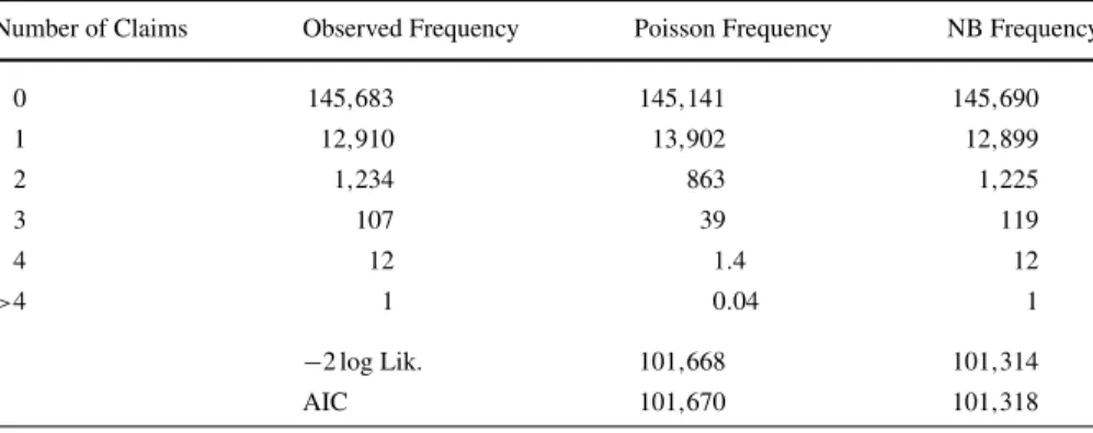
Illustration 2.2 (Negative binomial distribution for claim counts) The data from
Il-lustration2.1are reconsidered. We extend the analysis by fitting the NB distribution to the raw data. As demonstrated in Table2, the NB distribution provides for an im-proved fit of the empirical distribution of the claim frequencies.
Risk classification Including risk factors in the Poisson or NB distribution allows one to build classification systems for the frequency component of the data. This is done with regression techniques. The expressions given below are for cross-sectional data with sample sizem.
– Poisson regression: specify a log–linear structure for the mean, namely λi =
exp(xiβ), then logL(β)= m i=1 nixiβ−exp(xiβ)−log(ni!) ; (9)
Table 2 Empirical distribution and Poisson and NB fit for claim frequencies from the Illustration2.1data Number of Claims Observed Frequency Poisson Frequency NB Frequency
0 145,683 145,141 145,690 1 12,910 13,902 12,899 2 1,234 863 1,225 3 107 39 119 4 12 1.4 12 >4 1 0.04 1 −2 log Lik. 101,668 101,314 AIC 101,670 101,318 1X∼(α, β)meansf X(x)= β α (α)xα−1e−βx.
– NB regression: for the specification in (8) E[Y] =μ and regression models can be built throughμi=exp(xiβ). OrNi ∼Poi(λiθ )withλi =exp(xiβ)andθ∼
(τ/μ, τ/μ), which leads to Pr[Ni=ni] = (α+ni) (α)ni! α λi+α α λi λi+α ni , (10)
withα:=τ/μ. Both approaches are similar.
Using these expressions, maximum-likelihood and Bayesian estimation are straightforward. The advantage of using Bayesian statistics is that one can simulate from the posterior distribution ofNi, conditional on the risk characteristics. Besides
the expected value, other summary measures can be calculated for this posterior dis-tribution. This enables the application of a whole range of premium principles.
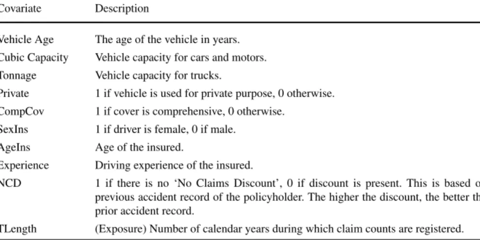
Illustration 2.3 (Regression models for claim counts) Using covariate information
a risk classification system is built for the data from Illustration2.1. The risk vari-ables used in the construction of this a priori model are enumerated in Table3. Their categorization is in Table14. Corresponding parameter estimates are in Table14at the end of this article. Selected risk profiles and their corresponding a priori premium (i.e. E[Ni]) are in Table4. Exposure for these profiles is assumed to be one full year.
A description of these profiles are given following the table below. Note that the variables ‘Age of insured’ and ‘Driving experience’ may be strongly correlated and, for reasons of multicollinearity, it may not be possible to retain both variables in the same regression model. In this example however, both had a significant effect on the response and, for a particular age, insureds with driving experiences between 0 and age-18years could be observed.
– Low: a 45 years old male driver with a driving experience of 19 years and a NCD=40. He’s driving a 1,166 cc Toyota Corolla that is 22 years old. He only has a theft cover. The car is for private use.
Table 3 List of explanatory variables used for the data in Illustration2.1 Covariate Description
Vehicle Age The age of the vehicle in years. Cubic Capacity Vehicle capacity for cars and motors. Tonnage Vehicle capacity for trucks.
Private 1 if vehicle is used for private purpose, 0 otherwise. CompCov 1 if cover is comprehensive, 0 otherwise.
SexIns 1 if driver is female, 0 if male. AgeIns Age of the insured.
Experience Driving experience of the insured.
NCD 1 if there is no ‘No Claims Discount’, 0 if discount is present. This is based on previous accident record of the policyholder. The higher the discount, the better the prior accident record.
Table 4 A priori risk premium
for a selection of risk profiles Risk Profile Poisson Distribution NB Distribution
Low 0.0460 0.0454
Medium 0.1541 0.1541
High 0.3727 0.3732
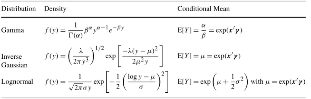
Table 5 A summary of some severity distributions considered in this section
Distribution Density Conditional Mean
Gamma f (y)= 1 (α)β αyα−1e−βy E[Y] =α β=exp(x γ) Inverse Gaussian f (y)= λ 2πy3 1/2 exp −λ(y−μ)2 2μ2y E[Y] =μ=exp(xγ) Lognormal f (y)=√ 1 2π σ yexp −12 logy−μ σ 2 E[Y] =exp μ+1 2σ 2withμ=exp(xγ)
– Medium: a 43 years old male driver with a driving experience of 11 years and a NCD=50. He’s driving a 1,995 cc Nissan Cefiro that is 2 years old. He has a comprehensive cover and the car is for private use.
– High: a 21 years old male driver with a driving experience of 3 years and a NCD=0. He’s driving a 1,597 cc Nissan that is 4 years old. His cover is com-prehensive and the car is for private use.
2.2.2 Claim severity models
Actuarial data on severities are (usually) positive and (very often) are skewed to the right, exhibiting a long right tail. Distributions from the exponential family suitable to model severity data are the Gamma and Inverse Gaussian distribution. After applying a log transformation to the losses, the Normal distribution is popular as well among practitioners. Specification of these distributions as members of the exponential fam-ily is documented in Kaas et al. (2008). In Illustration2.4risk classification based on these severity distributions is demonstrated. Covariate information is incorporated in the likelihood specifications according to the table summarized below.
Severity distributions from the GLM framework can be used to fit the whole data set with a single distribution. However, very often, when claim sizes are modeled, right tails heavier than those from the GLM framework are encountered. It is then useful to specify a mixture of distributions; one for the body of the data and another one for the tail. For the latter extreme value methods can be used (e.g. using Pareto-type modeling of the tail). See Beirlant et al. (2004) for an example demonstrating its usefulness using losses from a reinsurance company.
Illustration 2.4 (Severity models) We consider the severities corresponding to the
data analyzed in Illustration2.1. These severities are obtained as the ratio “aggre-gate loss/total number of claims” for each policyholderiand for each time period.
Table 6 Descriptive statistics of empirical distribution automobile insurance severity data
Mean StdDev Min 10% 25% 50% 75% 90% 97.5% 99.5% Max
4,439 7,100 1 610 1,229 2,575 5,337 9,835 19,205 37,344 306,304
Fig. 1 Automobile insurance
severity data; histogram and densities of gamma, Inverse Gaussian and lognormal
Fig. 2 Automobile insurance severity data; histogram, fitted Lognormal density and risk premium for
selected groups of insureds
Characteristics of these severities are displayed in Table6. Ignoring risk classifying information, the quality of the fit of the Gamma, Inverse Gaussian and Lognormal distributions to the data is illustrated in Fig.1.
The results of including risk classifying characteristics in these severity models are tabulated in Table15. Figure2compares the histogram of severities with the fitted Lognormal density for groups of insureds (based on risk classifying characteristics). For each group, the corresponding risk premium—determined as the expected value of the Lognormal distribution—is indicated with a vertical line.
2.3 Advanced models
Empirical distributions of claim counts often reveal an inflated number of zeros (i.e. no claim reported) and overdispersion (i.e. variance exceeding the mean). To cope with these characteristics, regression models beyond the Poisson and NB regression models are discussed in Sect.2.3.1. In addition, a typical feature of the empirical dis-tribution of claim severities is its right-skewness and long- or heavy-tailed character. To appropriately model such response variables, distributions outside the exponential family may be necessary. We provide two examples of flexible, parametric families of distributions, namely the Burr XII and Generalized Beta of the Second Kind (GB2). This is the topic of Sect.2.3.2.
2.3.1 Frequency models: generalized count distributions
The recent works of Yip and Yau (2005) and Boucher et al. (2007) in the actuarial literature highlight the use of parametric distributions other than the Poisson and the NB distributions to accommodate specific features of actuarial data. Cameron and Trivedi (1998), Winkelmann (2003), Yau et al. (2003), and Lee et al. (2006) similarly discuss regression modeling of data with excess zeros found in econometrics and medical statistics.
Mixtures The NB distribution was our first example of a mixture of the Poisson dis-tribution in this paper. Other continuous mixtures of the Poisson disdis-tribution that have been studied in the actuarial literature include, among others, the Poisson-Inverse Gaussian (‘PIG’) distribution and the Poisson-LogNormal (‘PLN’) distrib-ution. These and other types of mixture models may be found in Panjer and Willmot (1992).
Zero-inflation The use of a discrete or finite mixture to model count data, like a zero-inflated Poisson or a zero-inflated NB distribution, recently gained popularity in actuarial statistics. See, for example, Yip and Yau (2005), Boucher et al. (2007) for cross-sectional and Boucher et al. (2009) for longitudinal data. A zero-inflated distribution is a mixture of a standard count distribution with a degenerate distribution concentrated at zero. Its use is primarily motivated by the inflated number of zeros (i.e. no claims reported) commonly found in actuarial data for claim count statistics. Say Pr(Y=y|θ)is the standard count distribution (e.g. Poisson or NB) andp ∈ (0,1)denotes the extra proportion of zeros, then
Y ∼
0 with probabilityp,
Pr(Y=y|θ with probability 1−p. (11)
This gives the following distributional specification (with ‘ZI’ for zero-inflated)
PrZI(Y=y|p,θ)=
p+(1−p)Pr(Y=0|θ), y=0,
In countries where experience rating systems are operational, reporting a claim can generally increase the insurance premium in the following years. Policyholders there-fore have the tendency to avoid reporting all incurred claims, which motivates the presence of inflated probability mass at zero. Zero-inflated distributions take this into account.
Hurdle models The so-called hurdle models (Mullahy1986) provide another possi-bility to deal with extra zeros in empirical data. Hurdle models are two-part models that will be used here with the hurdle at zero. As such we discriminate between poli-cies with a claim and polipoli-cies without a claim. Zeros are then modeled as a binary component and non-zero observations with a truncated count distribution or a count distribution defined for strictly positive integers. Thus, when a truncated count distri-bution is used over the hurdle, we get
PrHur(Y=0|p,θ)=p,
PrHur(Y=y|p,θ)= 1−p
1−Pr(0|θ)Pr(Y=y|θ), y >0, (13)
wherepis the probability of zero claims and Pr(·)is the standard count distribution from which the truncated form 1−Pr1(0)Pr(Y=y)is derived. For a count distribution specified on the strictly positive integers, one similarly gets
PrHur(Y=0|p,θ)=p,
PrHur(Y=y|p,θ)=(1−p)Pr(Y=y), y >0. (14) Pr(·)now denotes a count distribution with the strictly positive integers as support.
As stated in Boucher et al. (2007), the belief that insureds behave differently when they already have reported a claim (as compared to when they are still claim free) motivates the use of a hurdle model with the hurdle at zero.
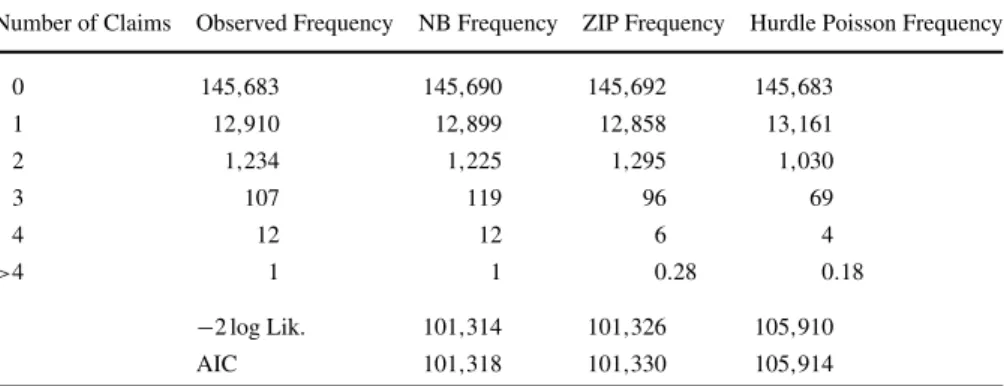
Illustration 2.5 (Generalized count distributions for claim counts) We now fit the
generalized count distributions discussed in this section to the data set introduced in Illustration2.1. Regression models based on these distributions are discussed in Illustration2.6.
Risk classification The inclusion of risk factors in the count distributions from Sect.2.3.1is done with regression techniques. The expressions given below are for cross-sectional data with sample sizen.
– Zero-inflated Poisson regression: use again a log-linear structure for the mean of the Poisson part and a logistic regression for the extra zeros. Thus,
logL(β,γ)= n i=1 uilog pi+(1−pi)exp(−λi) + n i=1 (1−ui)log (1−pi) exp(−λi)λyii yi! , (15)
Table 7 Empirical distribution and Negative Binomial, zero-inflated Poisson and hurdle Poisson fit for
claim frequencies corresponding to the data introduced in Illustration2.1
Number of Claims Observed Frequency NB Frequency ZIP Frequency Hurdle Poisson Frequency
0 145,683 145,690 145,692 145,683 1 12,910 12,899 12,858 13,161 2 1,234 1,225 1,295 1,030 3 107 119 96 69 4 12 12 6 4 >4 1 1 0.28 0.18 −2 log Lik. 101,314 101,326 105,910 AIC 101,318 101,330 105,914 wherepi= exp(ziγ)
1+exp(ziγ),λi=exp(xiβ)andui=I (yi=0). The log-likelihood then
becomes logL(β,γ)= n i=1 uilog
exp(ziγ)+exp−exp(xiβ)
+ n i=1 (1−ui) yixiβ−exp xiβ − n i=1
log1+exp(ziγ)−(1−ui)log(yi!) . (16)
– Hurdle Poisson regression:
logL(β,γ)= n i=1 uilog(pi)+(1−ui)log(1−pi) + n i=1 (1−ui) yilog(λi)−log 1−exp(−λi) −log(yi!)−λi , (17) where similarlypi= exp(ziγ)
1+exp(ziγ) andλi=exp(xiβ).
Illustration 2.6 (Regression models for claim counts) Illustration2.3is continued. Table14shows parameter estimates for a risk classification system based on the ZIP. Corresponding risk premiums are in Table8.
Table 8 A priori risk premium for a selection of risk profiles
Risk Profile Poisson distribution NB distribution ZIP distribution
Low 0.0460 0.0454 0.0455
Medium 0.1541 0.1541 0.1537
High 0.3727 0.3732 0.3715
2.3.2 Flexible, parametric models for claim severity
There are peculiar characteristics of insurance claim amounts such as skewness and heavy-tailness that usually cannot be accommodated by classes of distributions be-longing to the exponential family. Thus, modeling the severity of claims as a function of their risk characteristics, in the form of covariate information, may require statis-tical distributions outside those belonging to the GLM class. Principles of regression within other flexible parametric families of distributions are illustrated in this sec-tion. In particular, we find the GB2 class of distributions to be indeed quite flexible. Introduced in economics to model distributions of income by McDonald (1984), the GB2 class has four parameters that allow for this extreme flexibility and is able to accommodate covariates as used in Sun et al. (2008). A special case of the GB2 class is the Burr Type XII distribution. The work of Beirlant et al. (1998) introduces Burr regression in the actuarial literature.
Other flexible parametric models also appear in Klugman et al. (2008), many of which are tabulated in the appendix of the book. Several of these loss distributions can be similarly extendable for regression purposes. All these parametric models usu-ally try to fit the whole body of the data with a single distribution. In Sect.2.2.2an alternative approach was mentioned, mixing a distribution for the body with one for the tail.
Illustration 2.7 (Fire insurance portfolio) The cumulative distribution functions for
the Burr Type XII and the GB2 distribution are given, respectively by
FBurr,Y(y)=1− β β+yτ λ , y >0, β, λ, τ >0, (18) and FGB2,Y(y)=B (y/b)a 1+(y/b)a;p, q , y >0, a=0, b, p, q >0, (19) whereB(·,·)is the incomplete Beta function. If the available covariate information is denoted by x (1×p), it is straightforward to allow one or more of the parameters in (18) or (19) to vary with x. The result can be called a Burr or a GB2 regression model.
As an illustration of this approach, we consider a fire insurance portfolio (see Beir-lant et al.1998) that consists of 1,823 observations. We want to assess how the loss distribution changes with the sum insured and the type of building. Claims expressed as a fraction of the sum insured (‘SI’) are used as the response variable. Explanatory
Fig. 3 Fire Insurance Portfolio: residual QQ plots for Burr and GB2 regression
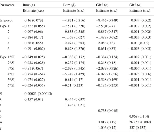
variables are the type of building and the sum insured. Residual Q–Q plots like those in Fig.3 are used to judge the goodness-of-fit of the proposed regression models. Details about the construction of these residual Q–Q plots can be found in the above-mentioned references. A summary of the resulting parameter estimates together with their respective standard errors are tabulated in Table9.
2.3.3 Additive regression models
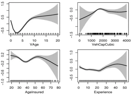
Thus far, only regression models with a linear structure for the mean, a transformation of the mean or a parameter in the distribution have been considered. Generalized additive models (GAMs) allow for more flexible relations between a response and a set of covariates. Without going into details, Fig.4shows the additive effect of the age of the vehicle (‘VAge’), its cubic capacity (‘VehCapCubic’) and the age of the driver (‘AgeInsured’) and his driving experience (‘Experience’) in a Poisson additive model with predictor
logμi=ηi=Exposure+β0+β1∗I (Sex=F)+β2∗I (NCD=0)
+β3∗I (Cover=C)+β4∗I (Private=1)+f1(VAge)
+f2(VehCapCubic)+f3(Experience)+f4(AgeInsured). (20) The model was fitted to the data from Illustration2.1. GAMs are an alternative for GLMs. As industry practice requires, our examples of GLMs use categorizations of continuous risk factors. An interesting feature of GAMs is that they provide insight
Table 9 Fire insurance portfolio: maximum-likelihood estimates and standard errors for Burr and GB2
regression models for observed losses. ‘SI’ stands for sum insured. For numerical reasons, losses are in 102for the Burr analysis and 103for the GB2 regression
Parameter Burr (τ) Burr (β) GB2 (b) GB2 (a) Estimate (s.e.) Estimate (s.e.) Estimate (s.e.) Estimate (s.e.) Intercept 0.46(0.073) −4.921(0.316) −8.446(0.349) 0.049(0.002) Type 1 −0.327(0.058) −2.521(0.326) −2.5(0.327) −0.012(0.002) 2 −0.097(0.06) −0.855(0.325) −0.867(0.317) −0.001(0.002) 3 −0.184(0.17) −1.167(0.627) −1.477(0.682) −0.003(0.003) 4 −0.28(0.055) −2.074(0.303) −2.056(0.3) −0.01(0.002) 5 −0.091(0.067) −0.628(0.376) −0.651(0.37) −0.003(0.003) Type 1*SI −0.049(0.025) −0.383(0.152) −0.384(0.154) −0.002(0.001) 2*SI 0.028(0.028) 0.252(0.174) 0.248(0.18) 0.001(0.001) 3*SI −0.51(0.067) −2.098(0.345) −2.079(0.326) −0.006(0.001) 4*SI −0.954(0.464) −5.242(1.429) −6.079(1.626) −0.025(0.006) 5*SI −0.074(0.027) −0.614(0.17) −0.598(0.169) −0.001(0.001) 6*SI −0.024(0.037) −0.21(0.223) −0.183(0.235) −0.001(0.001) β 0.00023(0.00013) λ 0.457(0.04) 0.444(0.037) τ 1.428(0.071) a 0.735(0.045) b 0.969 (0.114) p 3.817(0.12) 263.53 (0.099) q 1.006(0.12) 357 (0.132)
to the specification of meaningful categories. Denuit and Lang (2004) provides for an excellent discussion of ratemaking with additive regression models. At the same time these authors incorporate postcode information in their rating system. This involves concepts from spatial statistics, a topic which is outside the scope of this paper.
3 Risk classification and a posteriori rating
During the construction of an a priori tariff structure, not all important risk factors may be observable. This is usually the situation for a new policyholder or even an existing one where there may be insufficient information to account for as many im-portant risk factors to meet the homogeneity requirement of an efficient risk classi-fication system. As a result, tariff cells will not be completely homogeneous. Take the case of a driver insured in an automobile insurance, his aggressiveness behind the wheel and the swiftness of his reflexes to be able to avoid possible accidents are difficult to assess. However, as the driver’s claims history become more available to the insurer, this provides an additional, important revelation of the true riskiness of the policyholder. The insurer has the need to continually assess the efficiency of its risk classification scheme, and as such, the additional information provided by the
Fig. 4 Data from Illustration2.1: additive effects in a Poisson GAM as specified in (20)
history of claims as they emerge must be taken into account. Thus, a posteriori sta-tistical models are necessary in taking into account the history of reported claims and in adjusting the a priori premium accordingly.
Experience rating has a long tradition in actuarial science. It is a way to penalize ‘bad risks’ and reward ‘good risks’. Here we find that the premium for an insurance contract is calculated, after some claims history has been revealed, by accounting for both the experience of the individual policyholder together with that of the whole insurance portfolio to which the contract belongs. How much weight is assigned to the policyholder’s own experience is termed ‘credibility factor’ in actuarial science. In the statistics discipline, this revised estimate of the premium is based on what is called a ‘shrinkage estimator’. In actuarial science, this topic is called credibility the-ory and several works on this concept have appeared in the literature. Typically, we start with citation of the formulation of the classic actuarial credibility models devel-oped by Bühlmann (1967) and Bühlmann (1969), which provided the profession with a theoretical justification of the underlying principles of experience or a posteriori rating. Professionals and researchers extended his fundamental works in several di-rections, e.g. Jewell (1975) presented credibility models for hierarchically structured portfolios and Hachemeister (1975) combined concepts of a priori risk classification with credibility. For a detailed and recent overview of credibility in actuarial science, see Bühlmann and Gisler (2005).
When updating the a priori tariff based on historical claims, actuaries are clearly dealing with panel (or longitudinal) data. This is different from the cross-sectional setting in Sect.2.1and involves repeated measurement on a group of ‘subjects’ (in this case: policies or policyholders) over time. Since they share subject-specific char-acteristics, observations on the same subject over time often are substantively cor-related and require a different toolbox for statistical modeling. For instance, in the
case of a posteriori rating, we will use Generalized Linear Mixed Models (GLMMs) instead of the GLMs from Sect.2.2. GLMMs extend GLMs by including random effects in the linear predictor. The random effects do not only determine the correla-tion structure between observacorrela-tions on the same subject, but also take heterogeneity among subjects, due to unobserved characteristics, into account. Whereas the above-mentioned papers on credibility are theoretically oriented, contemporary statistical and econometric models for panel data and other types of clustered data allow the actuary to construct computationally driven a posteriori rating models, which can be implemented in standard statistical software packages. Throughout the various exam-ples, we present this kind of statistical tools for a posteriori rating. Useful references that discuss various aspects of a posteriori rating include, but are not limited to, Pin-quet (1997,1998), Frees et al. (1999), Pinquet et al. (2001), Bolancé et al. (2003) and Antonio and Beirlant (2007).
Apart from the time component of recorded data, it is possible that a company may have several other layers of observations. To illustrate, it is not uncommon to find an automobile insurer to provide “fleet” coverages where a single insurance policy cov-ers more than a single vehicle. Thus, the company has observations for a vehicle over a period of time under a “fleet” coverage. An additional level may be introduced when the observations are aggregated in the form of an “intercompany” experience, where the data comes from several companies. Such is usually the case for data obtained by reinsurers, companies that provide insurance protection to insurance companies. The analysis of data with such a multilevel structure is the topic of Sect.3.2.
Experience rating based on multilevel (panel or higher order) models as discussed in Sects.3.1and3.2poses a challenge to the insurer when it comes to communi-cating the predictive results of these models to the policyholders. Customers may find it difficult to understand. It is not readily transparent to an ordinary policyholder how the surcharges (maluses) for reported claims and the discounts (bonuses) for claim-free periods are evaluated. In order to establish an experience rating system where insureds can easily understand the effect of reported claims or periods without claims, Bonus–Malus scales have been developed. Examples of these are discussed in Sect.3.3.
3.1 A priori and a posteriori rating with credibility models for panel data
Continuing with our discussion of GLMs started in Sect.2.2, we now focus on ex-tending this type of models for a posteriori rating. GLMMs extend GLMs by allowing for random, or subject-specific, effects in the linear predictor (6). Including random effects in the linear predictor reflects the idea that there is a natural heterogeneity across subjects (policyholders, in this case) and that the observations on the same subject share common characteristics. This is the idea behind a posteriori ratemak-ing.
To fix ideas, suppose we have a data set consisting ofNsubjects. For each subjecti
(1≤i≤N)Tiobservations are available. Given the vectorbiwith the random effects
for subject (or cluster)i, the repeated measurementsYi1, . . . , YiTi are assumed to be
independent with a density from the exponential family
f (yit|bi,β, φ)=exp yitθit−ψ (θit) φ +c(yit, φ) , t=1, . . . , Ti. (21)
Similar to (6), the following (conditional) relations hold
μit=E[Yit|bi] =ψ(θit) and Var[Yit|bi] =φψ(θit)=φV (μit), (22)
whereg(μit)=xitβ+zit bi. As before,g(·)is called the link andV (·), the variance
function.β (p×1) denotes the fixed effects parameter vector (governing a priori rating) andbi (q×1) the random effects vector.xit (p×1) andzit (q×1)
con-tain subjecti’s covariate information for the fixed and random effects, respectively. The specification of the GLMM is completed by assuming that the random effects, bi (i=1, . . . , N), are mutually independent and identically distributed with density
functionf (bi|α). Herewithαdenotes the unknown parameters in the density. It is not uncommon to assume that the random effects have a (multivariate) normal dis-tribution with zero mean and covariance matrix determined byα. Dependence be-tween observations on the same subject arises because they share the same random effectsbi.
The likelihood function for the unknown parametersβ,αandφthen becomes L(β,α, φ;y)= N i=1 f (yi|α,β, φ)= N i=1 Ti t=1 f (yit|bi,β, φ)f (bi|α) dbi, (23)
wherey=(y1, . . . ,yN) and the integral is with respect to theq dimensional vec-torbi. For instance, when both the data and the random effects are normally
dis-tributed, the integral can be worked out analytically and explicit expressions exist for the maximum-likelihood estimator ofβand the Best Linear Unbiased Predictor (‘BLUP’) forbi. For more general GLMMs, however, approximations to the
likeli-hood or numerical integration techniques are required to maximize (23) with respect to the unknown parameters.
To illustrate the concepts described above, we now consider a Poisson GLMM with normally distributed random intercept. This GLMM allows for explicit calcu-lation of the marginal mean and covariance matrix. In this way, one can clearly see how in this example the inclusion of the random effect leads to overdispersion and within-subject covariance.
Illustration 3.1 (A Poisson GLMM) LetNit denote the claim frequency registered
in yeart for policyholderi. Assume that, conditional onbi,Nit follows a Poisson
distribution with mean E[Nit|bi] =exp(xitβ+bi)and thatbi∼N (0, σb2).
Straight-forward calculations lead to Var(Nit)=Var E(Nit|bi) +EVar(Nit|bi) =E(Nit)
exp(xitβ)exp3σb2/2−expσb2/2+1, (24) and Cov(Nit1, Nit2)=Cov E(Nit1|bi),E(Nit2|bi) +ECov(Nit1, Nit2|bi) =expxit1βexpxit2βexp2σb2−expσb2. (25)
Hereby we used the expressions for the mean and variance of a Lognormal distrib-ution. In the expression for the covariance we used the fact that, given the random effectbi,Nit1 andNit2 are independent. We see that the expression inside the
paren-theses in (24) is always bigger than 1. Thus, althoughNit|bifollows a regular Poisson
distribution, the marginal distribution ofNit is overdispersed. According to (25), due
to the random intercept, observations on the same subject are no longer independent.
Illustration 3.2 (A Poisson GLMM—continued) LetNit again denote the claim
frequency for policyholder i in year t. Assume that, conditional on bi, Nit
fol-lows a Poisson distribution with mean E[Nit|bi] =exp(xitβ+bi) and that bi ∼
N (−σ
2
b
2, σ 2
b). This re-parameterization is commonly used in ratemaking. Indeed, we
now get E[Nit] =E E[Nit|bi] =exp xitβ−σ 2 b 2 + σb2 2 =exp(xitβ), (26) and E[Nit|bi] =exp(xitβ+bi). (27)
This specification shows that the a priori premium, given by exp(xitβ), is correct on the average. The a posteriori correction to this premium is determined by exp(bi).
Besides the Lognormal distribution used in the above examples, other mixing dis-tributions can be used. In the Poisson-Gamma framework for instance, the conjugacy of these distributions allows for explicit calculation of the predictive premium. This is demonstrated in Illustration3.3.
Illustration 3.3 (A Poisson-Gamma model) A simple and classical random effects
Poisson model for panel data (see e.g. Hausman et al.1984) is constructed with the assumptions
Nit∼Poi(biλit), whereλit=exp(xitβ)andbi∼(α, α).
It follows thatE[bi] =1 and the resulting joint, unconditional distribution then
be-comes Pr(Ni1=ni1, . . . , NiTi=niTi) = T i t=1 λnit it nit! (Ti t=1nit+α) (α) α Ti t=1nit+α α × T i t=1 nit+α −Ti t=1nit ,(28)
with E[Nit] =E[E[Nit|bi]] =λit and Var[Nit] =E[Var[Nit|bi]] +Var[E[Nit|bi]] =
For the specification in (28), the posterior distribution of the random interceptbi
has again a Gamma distribution with
f (bi|Ni1=ni1, . . . , NiTi=niTi)∝ T i t=1 nit+α, Ti t=1 λit+α . (29) The (conditional) mean and variance of this posterior distribution are given, respec-tively, by E[bi|Nit=nit, t=1, . . . , Ti] = α+Ti t=1nit α+Ti t=1λit and (30) Var[bi|Nit=nit, t=1, . . . , Ti] = α+Ti t=1nit α+Ti t=1λit 2. (31)
This leads to the following a posteriori premium:
E[Ni,Ti+1|Nit=nit, t=1, . . . , Ti] =λi,Ti+1E[bi|Nit=nit, t=1, . . . , Ti] =λi,Ti+1 α+Ti t=1nit α+Ti t=1λit . (32)
The above credibility premium is optimal when a quadratic loss function is used. Indeed, as is known in mathematical statistics, the conditional expectation minimizes a mean squared error criterion.
It is now demonstrated how credibility calculations for a panel data set can be done with standard statistical software packages.
Illustration 3.4 (A numerical example of a posteriori rating with a Poisson GLMM)
We illustrate the statistical tools introduced above with a numerical example. Data consist of 12,893 policyholders who were observed during (fractions of) the period 1993–2003. LetNitbe the number of claims registered for policyholderiin periodt.
The following model specification is used:
Nit|bi∼Poi(μit|bi) and μit|bi=eitexp(xitβ+bi), (33)
bi∼N
−σ2/2, σ2, (34)
whereeit is the exposure for policyholderiin yeart(expressed in years). If the rating
model only uses observable risk characteristics (in xit) and not the claims history of
the insured, the a priori premium is given by
(a priori) E[Nit] =eitexp(xitβ). (35)
An experience rating system will adopt the a priori premium based on the claims reported by the insured. This results in the following a posteriori premium:
Fig. 5 (Left) Boxplot of the conditional distribution ofbi, given the historyNi1, . . . , NiTi, for a random
selection of 20 policyholders. (Right) For the same selection of policyholders: boxplots with simulations from the a priori (white) and a posteriori (gray) premium
The ratio (36)/(35) is called the theoretical Bonus–Malus Factor (BMF). It reflects the extent to which the policyholder is rewarded or penalized for his past claims. Using standard statistical software (likeProc NlMixedinSAS) a point estimate for (35), (36) and the BMF can be obtained easily. In Fig.5 (left) random draws from the conditional distributions ofbi(givenNi1, . . . , NiTi) are shown for a random
selection of policyholders. These results can be obtained from a Bayesian analysis of the model (using, for example,WinBugs). The conditional distributions reflect the heterogeneity between policyholders as well as their risk behavior. For instance, the black boxplot represents a policyholder who reported four claims during an insured period of 0.67 years, while the white boxplot represents a policyholder with zero claims during 6.4 years of exposure. The right panel of Fig. 5 shows boxplots of simulated values of the a priori ((35)) and a posteriori ((36)) premiums ofNi,Ti+1
(for the selection of policyholders under consideration). One can see how the a priori premiums are corrected based on observed claims.
More supporting graphs are given in Figs.6and7. Such graphs help the actuary to gain further insight into the portfolio. The vertical axis in both figures gives the a pos-teriori premium, expressed as a percentage of the a priori premium. The horizontal axis in Fig.6gives the average number of claims reported by the policyholder per year. This average is the ratio of total reported claims and the total period of exposure (in years). For instance, for the policyholders highlighted in Fig.6 (left panel) we observed four claims on 0.64 years (purple), two on 0.36 (years) (blue) and one on 0.167 year. These claim histories result in a posteriori 462%, 220% and 150% of the a priori premium. The right panel in Fig.6is a detail of the left panel. In this panel we only display policyholders with a total period of exposure of 3 years. For instance, the green triangles all represent policyholders who reported the same number of claims (i.e. one claim) during the same period of exposure (i.e. 3 years). Nevertheless, the a posteriori corrections that apply to this group of policyholders differ within the group. The dashed lines in the plot connect policyholders with a low (respectively
Fig. 6 A posteriori premium expressed as percentage of the a priori premium (y-axis) versus the average number of claims
Fig. 7 A posteriori premium expressed as percentage of the a priori premium (y-axis) versus the total period of insurance. Left panel uses the mean and right panel the median of the conditional distribution of
bi, givenNi1, . . . , NiTi
high) a priori risk premium. It becomes clear from the plot that corrections for high a priori risks are softer (i.e. penalties are lower and discounts are higher) than those for low a priori risks.
Figure7has the policyholder’s total exposure on thex-axis. In the left panel we use the mean of the conditional distribution ofbi (givenNi1, . . . , NiTi) as predictor
forbiin (36). The right panel uses the median. We see that the median results in a less
severe experience rating: smaller penalizations for past claims and bigger rewards for claim-free policies. At the same time Fig.7illustrates graphically how many claim-free years a policyholder needs to get rid of his penalty, e.g. after reporting one claim, and pay the a priori premium again. Graphically this is represented by the intersection of the green cloud and a horizontal line aty=100.
3.2 A priori and a posteriori rating with credibility models for clustered data Whereas Sect.3.1is an overview of techniques involved in the rating of data bases with a panel structure, actuaries may have data sets at their disposal with a more difficult structure. This is illustrated with an example of multilevel or hierarchical rating that first appeared in the actuarial literature in Antonio et al. (2010).
Illustration 3.5 (A multilevel model for intercompany claim counts) Data are available on claim counts registered for automobile insurance policies over a pe-riod of nine years (1993–2002). The source contains a pooled experience of several insurers. Moreover, vehicles under consideration are insured under a ‘fleet’ policy. Fleet policies are umbrella-type policies issued to customers whose insurance covers more than a single vehicle. The hierarchical or multilevel structure of the data is as follows: vehicles(v)observed over time (t )that are nested within fleets (f ), with policies issued by insurance companies(c). Multilevel statistical models allow one to incorporate the hierarchical structure of the data by specifying random effects at the vehicle, fleet and company levels. These random effects represent unobservable characteristics at each level. At the vehicle level, the missions assigned to a vehicle or unobserved driver behavior may influence the riskiness of a vehicle. At the fleet level, guidelines on driving hours, mechanical check-ups, loading instructions and so on, may influence the number of accidents reported. At the insurance company level, underwriting and claim settlement practices may affect claims. Moreover, random ef-fects allow one to update an a priori tariff, taking into account the past performance of vehicle, fleet and company. As such, they are relevant for a posteriori rating with clustered data.
Antonio et al. (2010) compare the performance of a posteriori rating models (in-corporating a priori characteristics) based on various count distributions (namely Poisson, negative binomial, zero-inflated Poisson and hurdle Poisson). DenoteYc,f,v,t
the number of claims in periodt for vehiclevinsured under fleetf by companyc. With the Poisson distribution the a priori tariff is expressed as
Nc,f,v,t∼Poi
μpriorc,f,v,t,
μpriorc,f,v,t=ec,f,v,texp(ηc,f,v,t), (37)
ηc,f,v,t=β0+xcβ4+xcfβ3+xcf vβ2+xcf vtβ1. (38) Herebyxc,xcf,xcf v andxcf vt contain observable covariate information registered
at the level of company, fleet, vehicle and period, respectively.ec,f,v,t denotes the
exposure. A posteriori the tariff is updated as follows:
Nc,f,v,t|bc;bc,f;bc,f,v∼Poi(μc,f,v,t|bc;bc,f;bc,f,v), μc,f,v,t|bc;bc,f;bc,f,v=μ prior c,f,v,t×exp(bc+bc,f+bc,f,v), (39) bc∼N −σc2 2 , σ 2 c and bc,f ∼N −σ 2 c,f 2 , σ 2 c,f and bc,f,v∼N −σ 2 c,f,v 2 , σ 2 c,f,v . (40)