DOCUMENTS DE TREBALL
DE LA FACULTAT DE CIÈNCIES
ECONÒMIQUES I EMPRESARIALS
Col·lecció d’Economia
Time of ruin in a risk model with generalized Erlang(n) interclaim
times and a constant dividend barrier
Maite Mármol
and
M. Mercè Claramunt
Adreça correspondència:
Departament de Matemàtica Econòmica, Financera i Actuarial Facultat de Ciències Econòmiques i Empresarials
Universitat de Barcelona Avda. Diagonal, 690 08034 Barcelona Tfn. 93 403 5744 Fax 93 403 7272
Abstract
In this paper we analyze the time of ruin in a risk process with the
interclaim times being Erlang(n) distributed and a constant dividend
barrier. We obtain an integro-differential equation for the Laplace
Transform of the time of ruin. Explicit solutions for the moments of the
time of ruin are presented when the individual claim amounts have a
distribution with rational Laplace transform. Finally, some numerical
results and a compare son with the classical risk model, with interclaim
times following an exponential distribution, are given
Resumen:
En este artículo analizamos el momento de ruina en un proceso del riesgo
donde el tiempo de ocurrencia entre los siniestros se distribuye según una
Erlang(n) y con una barrera de dividendos constate. Obtenemos una
ecuación integro diferencial para la Transformada de Laplace del momento
de ruina.
Presentamos soluciones explicitas para el momento de ruina cuando la
cuantía individual de un siniestro cumple que la Transformada de Laplace
de su función distribución es racional. Finalmente, se muestran resultados
numéricos y una comparación con el modelo clásico (con tiempos de
interocurrencia exponencial)
Keywords:
Risk theory, Generalized Erlang (n) distribution, constant
dividend barrier, time of ruin, Laplace Transform
1
Introduction
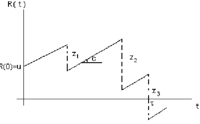
In the classical model of risk theory, the insurer’s surplus process at a given time t, R(t), is given by R(t) =u+c·t− N(t) X i=1 Zi , t∈[0,∞)
with u = R(0) being the insurer’s initial surplus. N(t), the number of claims occurred until time t, follows a Poisson process with parameter λ,
and Zi is the amount of the i-th claim and has density function f(z). The instantaneous premium rate, c, isc=E[N]·E[Z]·(1 +ρ), whereρ, called the security loading, is a positive constant.
Figure 1: Sample path for the classical risk process
Define τ to be the time of ruin so that τ = inf{t :R(t)<0}, with
τ = ∞ if R(t) ≥ 0 for all t > 0. We denote the ultimate ruin probability from initial surplus uby ψ(u), so that ψ(u) =P[τ <∞]. The time to ruin in the classical risk model is considered in Gerber and Shiu (1998), Lin and Willmot (2000), Dickson and Waters (2002), Drekic and Willmot (2003), or Ren (2005) where a perturbed model is analyzed.
In this paper the Poisson number process of the classical risk model is replaced with a more general renewal risk process with inter-occurrence times of a General Erlang(n) type. The time of ruin in an Erlang risk process is considered in Albrecher et al. (2005), Dickson and Hipp (2001) and Dickson et al. (2003) and Li and Garrido (2004) where an integro-differential equation for the Gerber-Shiu function is derived.
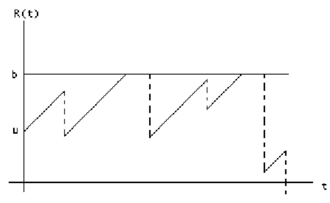
In what follows we shall use the modified model with a constant divi-dend barrier b , 0 ≤ u ≤ b, so that when the surplus reaches the level b, premium income is paid out as dividend to shareholders and the modified surplus process remains at level buntil the occurrence of the next claim. In this model the probability of ruin is equal to one, so we can assure that τ <∞.
Figure 2: Modified model with a constant dividend barrier
The layout of this paper is as follows. In the next section we obtain the integro-differential equation for the Laplace transform of the time of ruin,
φ(u), in a model modified with a constant dividend barrier in a Sparre Andersen model with generalized Erlang(n) interclaim times. Using rational Laplace Transforms, we solve the corresponding differential equation.
Section 3 presents the results for the particular case when the interclaim time follows an Erlang(2, λ)process. In 3.1 we obtain the boundary condition
when the individual claim amount is distributed as an exponential distrib-ution, and in 3.2 when the individual claim amount follows an Erlang(2, β)
distribution.
In section 4 some ideas about the interpretation of the Laplace transform are given, and by differentiating φ(u) we will obtain the n-moments of the time of ruin and some numerical results are presented. Finally a comparison with the classical risk model is presented.
2
Laplace Transform of the time of ruin
We start by obtaining the integro-differential equation for the Laplace Trans-form of the time of ruin. We define,
φ(u) =E£e−δτ¤.
We assume that the interocurrence timesTi, i= 1,2, ..follow a generalized Erlang(n) distributed, i.e. each Ti is a sum of n independent exponential random variables with possibly different parameters λ1, ..., λn each causing a "sub-claim" of size 0 and at the time of the nth subclaim a claim with distribution F occurs. We consider n states of the risk process (starting at time 0 in state 1) , where every subclaim causes a transition to the next state and in the time of occurrence of thenthsubclaim the risk process jumps into state 1 again (see Albrecher at al. (2005)).
Let φj(u) denote the Laplace transform of the time of ruin if the risk process is in state j = 1, ..., n.
Theorem 1 The integro-differential equation for φ(u) is,
à n Y j=1 µ δ+λj−c∂· ∂u ¶! φ(u)− n Y j=1 λj Z u 0 φ(u−z)dF(z)− n Y j=1 λj[1−F (u)] = 0, (1)
with boundary condition, k−1 Y j=1 Ã δ+λj−c∂· ∂u λj ! ∂φ(u) ∂u ¯ ¯ ¯ ¯ u=b = 0 for k = 1, ..., n (2)
Proof. For 0≤u < b, by differential argument
φj(u) = (1−λjdt)φj(u+cdt)e−δdt+
λjdtφj+1(u+cdt)e−δdt+θ(dt) for j = 1, ..., n−1 (3)
beeing θ(dt) the probability of more than one claim occurs in dt.
φn(u) = (1−λndt)φn(u+cdt)e−δdt+ λndtR0u+cdtφ1(u+cdt−z)dF(z)e−δdt+ λndte−δdtR∞ u+cdtdF(z) +θ(dt) forj =n (4) Then by linear approximation, dividing by dt, and taking dt → 0, from
(3) and(4)we obtain, c∂φ j (u) ∂u −(δ+λj)φ j (u) +λjφj+1(u) = 0, for j = 1, ..., n−1. (5) c∂φ∂un(u)−(δ+λn)φn(u) + λnR0uφ1(u−z)dF(z) +λn[1−F (u)] = 0. forj =n (6) From(5), φj+1(u) = Ã (δ+λj)−c∂u∂· λj ! φj(u), j = 1, ..., n−1,
and following a recursive process, φn(u) = Ãn−1 Y j=1 (δ+λj)−c∂u∂· λj ! φ1(u). (7)
We can write(6)as,
µ (δ+λn)−c∂· ∂u ¶ φn(u)−λn Z u 0 φ1(u−z)dF(z)−λn[1−F (u)] = 0. (8) Substituting(7)in (8),(1) is obtained.
Foru=busing an analogous process for j = 1, ..., n−1
φj(b) = (1−λjdt)φj(b)e−δdt+λjdtφj+1(b)e−δdt+θ(dt)
we obtain
λjφj+1(b)−(δ+λj)φj(b) = 0
that comparing with (5),
∂φj(u) ∂u ¯ ¯ ¯ ¯ u=b = 0 (9) And forj =n, φn(b) = (1−λndt)φn(b)e−δdt+λndtRb 0 φ 1(b −z)dF(z)e−δdt+ λndte−δdtR∞ b dF(z) +θ(dt) then, λn Z b 0 φ(b−z)dF(z) +λn Z ∞ b dF(z)−(δ+λn)φn(b) = 0
and comparing with (6)
∂φn(u) ∂u ¯ ¯ ¯ ¯ u=b = 0 (10)
Using an alternative method, Li and Garrido (2004) obtained an equiv-alent integro-differential equation and boundary conditions for the Gerber-Shiu function.
Applying Laplace transforms to(1) we obtain,
ϑ(s)eφ(s) +Ln−1(s)− n Y j=1 λj à e φ(s)fe(s)− 1−fe(s) s ! = 0, (11)
being eφ(s) the Laplace transform of φ(u) and fe(s) the Laplace transform of the claim density function f(z).
Ln−1(s) represents the n−1 degree polynomial, whose coefficients
in-volve the quantities ∂φ∂uj)(u)
¯ ¯ ¯
u=0 , j = 0, ..., n−1, and ϑ(s) is the n degree
polynomial ϑ(s) = n Y j=1 (δ+λj −cs). From(11) we obtaineφ(s), e φ(s) = n Y j=1 (λj)³1−fsh(s)´−Ln−1(s) ϑ(s)− n Y j=1 λjfe(s) . (12)
Example 2 Assuming the classical model of risk theory with interocurrence
claims Erlang(1, λ), expression (12) is,
e
φ(s) =
λ³1−fsh(s)´−cφ(0)
(δ+λ−cs)−λfe(s). (13)
Let us now restrict the further analysis to the case of claim size distribu-tion with radistribu-tional Laplace transform
e
f(s) = Qr−1(s)
wherePr(s)and Qr−1(s)denote polynomials of degreer and (at most)r−1
respectively with no common zeros. Moreover Pr(s) has leading coefficient 1, no roots in the positive half plane andPr(0) =Qr−1(0).For this claim size
distribution, the denominator of (12)hasn+rzeroes, which ares1, ..., sn+r.,
and we assume that the roots are real and distinct. From the above we conclude that r of these zeroes are located in the negative halfplane. Then using partial fractions, it is obtained,
φ(u) =
n+r
X
i=1
αi(b)esiu. (14)
Note that αi(b) are functions of b, but for brevity we writeαi. Now, we need to find n+r equations satisfied by αi, i = 1, ..., n+r. The first n are obtained from (2).
3
Laplace transform of Time of ruin in Erlang
(2
, λ
)
risk model
Assuming the case of a Sparre Andersen model with Erlang(2, λ) interclaim times (n= 2 andλ1 =λ2 =λ) the integro-differential equation forφ(u) is
µ δ+λ−c∂· ∂u ¶2 φ(u)−λ2 Z u 0 φ(u−z)dF(z)−λ2[1−F(u)] = 0, (15)
From(12), it is easy to obtain
e
φ(s) =
λ2³1−fsh(s)´+c2φ0(0) + (c2s
−2c(δ+λ))φ(0)
(δ+λ−cs)2−λ2fe(s) , (16)
ob-tained φ(u) = 2+r X i=1 αi(b)esiu. (17)
3.1
Claim distribution
z
∼
exp (
γ
)
If we assume that f(z) = γe−γz, then fe(s) = γ
γ+s. We obtain the roots si, i= 1,2,3, from
(δ+λ−cs)2(γ+s)−λ2γ = 0. (18)
Then the solution ofφ(u) is,
φ(u) =
3
X
i=1
αiesiu. (19)
Thefirst two equations obtained from(2)are
3 X i=1 siαiesib = 0and 3 X i=1 s2iαiesib = 0.
To find the third equation, we substitute (19) and f(z) = γe−γz in the
integro-differential equation (15), and resolving the integral,
3 X i=1 αiesiu ∙ (λ+δ)2−2c(λ+δ)si+c2s2i − λ 2γ (si+γ) ¸ + λ2γ 3 X i=1 αie−γu (si+γ) −λ 2 e−γu= 0.
From (18)the coefficient ofesiu is equal to zero, then we obtain the third
equation, 3 X i=1 αi (si+γ) = 1 γ.
We thus have a system of three equations from which we can easily solve for αi, i= 1,2,3 using Mathematica.
3.2
Claim distribution
z
∼
Erlang
(2
, β
)
Consider a risk process in which claims occur as an Erlang(2, β)distribution,
f(z) =β2ze−βz with Laplace transformfe(s) = (β+s)β2 2.Then the fourth roots
are obtained from
(δ+λ−cs)2(β+s)2 −λ2β2 = 0 (20)
The solution in this case is,
φ(u) =
4
X
i=1
αiesiu. (21)
We need tofind four equations to calculate the unknownsαi, i= 1,2,3,4.
Two equations are obtained from (2):
4 X i=1 siαiesib = 0and 4 X i=1 s2 iαiesib = 0.
From(15),(21)and knowing thatf(z) =β2ze−βz, wefind the other two, 4 X i=1 αi (si+β)2 = 1 β2 and 4 X i=1 αi (si+β) = 1 β.
4
Getting information from Laplace transform
of the time of ruin
From φ(u) we can get two kind of different informations about the time of ruin.
First φ(u) = E£e−δτ¤ can be interpreted as the expected present value
of one monetary unit that was paid at the time of ruin. Then the parameter of the Laplace transform δ can be interpreted as the interest rate used to
obtain the present value.
But alsoφ(u)allows us tofind the the n-moments of the random variable
τ, i.e. E[τn],that can be obtained differentiatingφ(u) with respect toδ,
∂nφ(u) ∂δn = ∂n ∂δnE £ e−δτ¤=E£(−τ)ne−δτ¤.
and evaluating these at δ = 0,
E[τn] = (−1)n ∂φ n (u) ∂δn ¯ ¯ ¯ ¯ δ=0 .
In what follows, some numerical results are obtained.
If we assume thatf(z) =γe−γz,forγ = 1, λ= 1, b= 10and c= 0.6,the results for E[τ], σ[τ] and the variation coefficient of τ defined by cv[τ] =
100.σ[τ]
E[τ] are summarized in Table 1,
E[τ] σ[τ] cv[τ] u= 0 93.9577 217.63 231.625 u= 1 157.031 265.267 168.926 u= 2 205.805 288.281 140.075 u= 3 243.077 299.847 123.355 u= 4 271.099 305.565 112.714 u= 5 291.68 308.253 105.682 u= 6 306.277 309.411 101.023 u= 7 316.06 309.845 98.0336 u= 8 321.974 309.973 96.2727 u= 9 324.794 309.996 95.4437 u= 10 325.372 309.997 95.2744 Table 1: E[τ], σ[τ]andcv[τ] forf(z) =e−z, λ= 1, b = 10and c= 0.6
Graphically, 2 4 6 8 10 u 100 150 200 250 300 E@τD
Figure 3: E[τ] assumingTi ∼Erlang(2,1)
and Z ∼ exp(1) 2 4 6 8 10 u 240 260 280 300 α@τD
Figure 4: α[τ] assuming Ti ∼Erlang(2,1)
and Z ∼ exp(1 2 4 6 8 10 u 100 120 140 160 180 200 220 cv@τD
Figure 5: cv[τ] assumingTi ∼Erlang(2,1)
4.1
Comparison with the classical model
In this section we are going to compare the time of ruin with a constant barrier in an Erlang risk model with the corresponding in the classical risk model.
In the classical risk model, claims occur as a Poisson process. Note that in a Poisson process with parameterλ,Ti, i≥1has an exponential distribution with mean λ1,i.e. with an Erlang(1, λ)distribution. So the time of ruin in the classical risk model is included in Theorem 1 as a particular case. From (1), for n= 1, we get the integro-differential equation for the Laplace transform of the time of ruin in the classical risk model and the boundary condition,
(δ+λ)φ(u)−cφ0(u)−λ Z u 0 φ(u−z)dF(z)−λ[1−F (u)] = 0 (22) ∂φ(u) ∂u ¯ ¯ ¯ ¯ u=b = 0.
This equation can be obtained too from equation (2.5) in Lin et al (2003) for the Gerber-Shiu function in the classical risk model. (See too Dickson and Waters (2004))
To solve this model, from (13), assuming that f(z) = γe−γz, the roots
are obtained from −c2s2+ (δ+λ
−cγ)s+δγ = 0. Thenφ(u) =
2
X
i=1
αiesiu.
To calculate αi, substitutingφ(u) =
2
X
i=1
αiesiu andf(z) =γe−γz in (22) we
get 2 X i=1 αi (si+γ) = 1 γ.
In order to analyze the influence that the distribution of the interclaim times has in the time of ruin, the two models have to be comparable, i.e.
E[Nt]whent→ ∞must be assimptotically the same in the Erlangian model and in the classical model.
Following Cox (1962), in an ordinary renewal process the renewal func-tion, E[Nt], is related withTi
e L(s) = 1 s e gTi(s) 1−egTi(s) , foregTi(s)<1
beingLe(s)the Laplace transform ofE[Nt]andegTi(s)the Laplace transform
of the density function of the interrocurrence times.
For an Erlangian model, i.e. Ti ∼ Erlang(n, λ) with egTi(s) =
¡ λ λ+s ¢n , then e L(s) = λ n s((λ+s)n−λn). (23)
From (23), if Ti ∼ Erlang(2, λ), E[Nt] is easily obtained inverting Le(s) =
λ2 s¡(λ+s)2−λ2¢,then E[Nt] = 1 E[Ti]t− 1 4 + 1 4e − 4 E[Ti]t.
From (23), if Ti ∼ Erlang(1, λ), i.e. for the classical risk model with
E[Ti] = 1
λ, Le(s) = λ
s2 and inverting, we have E[Nt] = t E[Ti].
So, ifE[Ti]is the same, the renewal functionE[Nt]has the same behavior whent → ∞.In general in an ordinary renewal process lim
t→∞ E[Nt] t = 1 E[Ti] (see Parzen (1972))
It´s easy to see also that the security loading included in the premium is different in the two models, and that if E[Ti] is the same, asymptot-ically the security loading in the two models coincides: It´s known that the total premium income until time t is ct = E[Z]E[Nt] (1 +ρt), then ρt =
ct
E[Z]E[Nt]−1, and assumingE[Z] = 1, for the Erlangian model
ρt= ct 1 E[Ti]t− 1 4 + 1 4e − 4 E[Ti]t −1
and for the classical model
ρt=cE[Ti]−1
Then, in order to compare the time of ruin in theErlang(2,1)model with
E[Ti] = 2with the classical model, where the interocurrence time follows an exponential distribution, the parameter of the exponential must be 0.5, i.e.
Ti ∼exp(0.5)with E[Ti] = 2.
The difference betweenE[τ]in the Erlang(2,1) model and in the classical model with Ti ∼ Exp(0.5) is represented in Figure 6. In the Figures 7 and Figure 8 the difference for σ[τ] and the variation coefficient of τ is repre-sented, 2 4 6 8 10 u 50 60 70 80 90 100 110 Difference E@τD
Figure 6: EErlang[τ]− EExp[τ]
2 4 6 8 10 u 90 95 100 105 110 Difference α@τD
2 4 6 8 10 u -15 -12.5 -10 -7.5 -5 -2.5 Difference cv@τD
Figure 8: cvErlang[τ]− cvExp[τ]
References
[1] Albrecher,H., Claramunt, M.M and M. Mármol (2005), "On the distrib-ution of dividend payments in a Sparre Andersen model with generalized Erlang(n) interclaim time" Insurance: Mathematics & Economics, 37, 324-334.
[2] Cox, D.R. (1962). "Renewal theory" Chapman and Hall. London. [3] Dickson,D.C.M and C. Hipp (2001),. "On the time to ruin for Erlang(2)
risk processes" Insurance: Mathematics & Economics,29,333-334. [4] Dickson,D.C.M., Hughes, B. and L. Zhang (2003), "The density of the
time to ruin for a Sparre Andersen process with Erlang arrivals and exponential claims" Centre for Actuarial Studies Research Paper Series N0 111. University of Melbourne.
[5] Dickson,D.C.M and H.R. Waters (2002), "The distribution of the time to ruin in the classical risk model" ASTIN Bulletin,32, 299-313.
[6] Dickson,D.C.M and H.R. Waters (2004), "Some optimal dividend prob-lems" ASTIN Bulletin, 34, 49-74.
[7] Drekic, S. and G.E. Willmot (2003), "On the density and moments of the time to ruin with exponential claims" ASTIN Bulletin,32, 11-21. [8] Gerber, H.U. and E.S.W Shiu (1998), "On the time value of ruin" North
American Actuarial Journal, 2, N0 1, 48-78.
[9] Li, S. and J. Garrido (2004) "On a class of renewal risk models with a constant dividend barrier" Insurance: Mathematics & Economics, 35, 691-701.
[10] Lin,S.X. and E. W. Gordon, (2000), "The moments of time of ruin, the surplus before ruin, and the deficit at ruin"Insurance: Mathematics & Economics, 27, 19—44.
[11] Lin,S.X, Gordon, E. W. and S. Drekic (2003), "The classical risk model with a constant dividend barrier: analysis of the Gerber—Shiu discounted penalty function" Insurance: Mathematics & Economics,33,551-566 [12] Parzen, E. (1972), "Procesos Estocásticos" Paraninfo. Madrid.
[13] Ren, J. (2005), "The expected value of the time of ruin and the moments of the discounted deficit at ruin in the perturbed classical risk process"