Journal of Computational Physics

Analytic Hessian derivation for the quasi-one-dimensional Euler equations

Eyal Arian

a

, Angelo Iollo

b,*

a

Computational Mathematics, The Boeing Company, MC 7L-21 P.O. Box 3707, Seattle, WA 98124-2207, USA b

Institut de Mathématiques de Bordeaux, UMR 5251 CNRS, Université Bordeaux 1, INRIA Bordeaux Sud-Ouest, Equipe-Projet MC2, 33405 Talence cedex, France

a r t i c l e

i n f o

Article history: Received 6 March 2008

Received in revised form 8 September 2008 Accepted 24 September 2008

Available online 10 October 2008

Keywords: Hessian Adjoint

Compressible Euler equations

a b s t r a c t

The Hessian for the quasi-one-dimensional Euler equations is derived. A pressure minimi-zation problem and a pressure matching inverse problem are considered. The flow sensi-tivity, adjoint sensisensi-tivity, gradient and Hessian are calculated analytically using a direct approach that is specific to the model problems. For the pressure minimization problem we find that the Hessian exists and it contains elements with significantly larger values around the shock location. For the pressure matching inverse problem we find at least one case for which the gradient as well as the Hessian do not exist. In addition, two formu-lations for calculating the Hessian are proposed and implemented for the given problems. Both methods can be implemented in industrial applications such as large scale aerody-namic optimization.

Ó2008 Elsevier Inc. All rights reserved.

1. Introduction

Aerodynamic optimization problems are computationally massive and highly ill-conditioned. In the past two decades they have matured and are now an integral part of design in the aerospace industry. Mathematically these are optimal design problems governed by partial differential equations. In this work we assume that the initial guess of the shape design prob-lem is in the basin of attraction of the desired global minimum, and therefore local gradient methods can be used to pursue the optimal solution. Jameson[1]introduced the idea of using Computational Fluid Dynamics (CFD) to solve the direct and adjoint flow models. By the adjoint method, the solution of a single adjoint problem allows to determine the gradient of an objective function with respect to the design parameters, regardless of the dimension of the design space. Beux and Dervieux [2]first gave examples of compressible flow shape derivatives computed by the adjoint of the discrete operator on unstruc-tured meshes. Frank and Shubin[3]considered several shape optimization strategies and took as a test case the quasi-one-dimensional compressible Euler equations. Iollo and Salas[4]studied the case of flows with shocks. They found that a bound-ary condition at the shock is needed for the adjoint equation. Giles and Pierce[5]determined this boundary condition and the analytical adjoint solution for the quasi-one-dimensional compressible flow in a nozzle. Additional references and a more complete review can be found in[6].

In most practical scenarios quasi-Newton methods are used in combination with the adjoint method (or sensitivity equa-tion method) to compute the search direcequa-tion. However, for large scale ill-condiequa-tioned problems quasi-Newton methods are slow at the start, and may take many iterations to build a good Hessian approximation. In practice it may not be affordable to allow enough iterations for the quasi-Newton to reach a good Hessian approximation, resulting in poor convergence. An approximation of the Hessian that is constructed from the governing equations and the objective function, can serve as a starting point for quasi-Newton methods. Such an initial approximation will be much more accurate than the identity matrix

0021-9991/$ - see front matterÓ2008 Elsevier Inc. All rights reserved. doi:10.1016/j.jcp.2008.09.021

* Corresponding author.

E-mail address:[email protected](A. Iollo).

Contents lists available atScienceDirect

Journal of Computational Physics

that is used by default in practice. Also, other preconditioning techniques (not based on quasi-Newton) can be devised based on the Hessian form.

A good Hessian approximation is important in particular for large scale industrial optimal design problems where the governing equations are solved using CFD. The Hessian for such problems is typically highly ill-conditioned as analyzed for example by Arian and Ta’asan in[7]. The gradient serves as a very poor search direction, while the gradient pre-multi-plied by the approximated inverse of the Hessian serves as an excellent search direction close enough to the solution as dem-onstrated by Arian and Vatsa in[8]. However, the techniques used in[7] and [8]are not practical in the industrial setting in which the governing state equations are more difficult to analyze. In practice we would like to use the available resources, such as sensitivities and adjoint solutions, to generate an approximated Hessian numerically.Another approach is to use automatic differentiation tools to generate the Hessian in the discrete level automatically (more details can be found in [9,10]).

In this paper we compute the Hessian analytically for two minimization problems governed by the quasi-one-dimen-sional Euler equations. An analytical form may reveal many unknowns on such problems, e.g., does the Hessian exist for transonic flow with a shock? What is the effect of the shock on conditioning? We examine three different methods to build the Hessian. The first method, called ‘‘the direct approach” in this paper, is specific to the problem at hand. Using the direct approach the analytical Hessian is derived for a transonic flow with a shock. The two additional methods are based on the adjoint and sensitivity equations, and can be applied in practice for large scale aerodynamic optimization problems. We demonstrate the application of these methods for supersonic flow and show numerically that all three methods result in the same Hessian matrix (up to a small truncation error). The two adjoint based methods have different computational cost. A preliminary analysis shows that one method might be numerically unstable when shocks are present in the flow. The method that is likely to be more stable is also more computationally intensive.

Our point of departure is the paper by Giles and Pierce[5]. In that paper the adjoint solution is derived analytically using Green’s function technique. We recover the adjoint solution in[5]and in addition compute the sensitivity solutions.

We present results for two different objective functions. The first is a standard pressure minimization objective function as considered in[5]. The second corresponds to an inverse problem in which the difference inL2_{norm between the pressure} and a given, target, pressure distribution is to be minimized.

The paper is organized as follows:

In Section2the mathematical formulation is presented.

In Section3the direct approach is discussed and key observations are made regarding the existence of the Hessian in the presence of a shock.

In Section4computational results of the direct method are discussed. In Section5the two adjoint based methods are derived.

In Section6numerical results of the adjoint based methods are presented for supersonic flow conditions. In Section7the paper is concluded with a discussion.

2. Formulation

The state variable,U, is defined to be the triplet composed of the density, mass flux, and total energy density: U¼ ð

q

;

q

q;

q

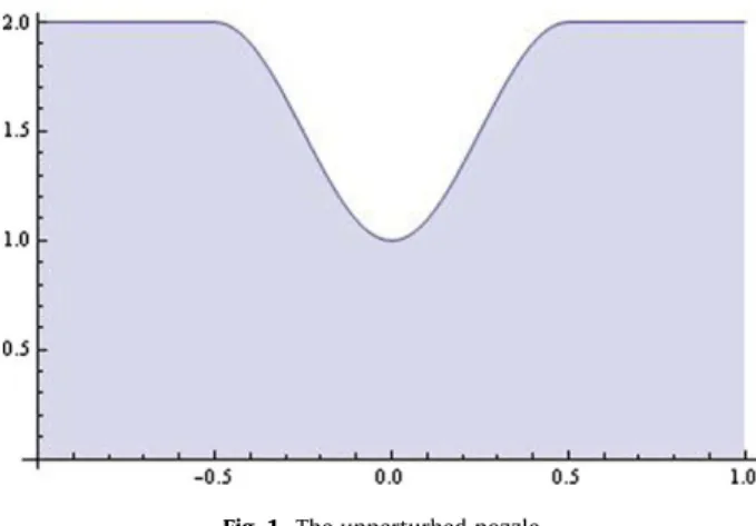
EÞT:

We consider the compressible Euler equations in a quasi-one-dimensional approximation. The flow takes place inside a noz-zle of heighthðxÞ, wherexis the spatial coordinate (seeFig. 1). The optimal design problem consists of minimizing an objec-tive function,JðUÞ, subject to state equations:

min hðxÞ JðUÞ RðU;hÞ ¼0 ð 1Þ with RðU;hÞ ¼ d dxðhFÞ dh dxP; ð2Þ and F¼ ð

q

q;

q

q2 þp;

q

HqÞT; P¼ ð0;p;0Þ;

wherepis the static pressure, and

q

His the total enthalpy density.

In this paper the objective function is defined to be either the integral of the pressure distribution across the domain

XR

JðUÞ ¼

Z

X

pdx: ð3Þ

or theL2norm of a pressure difference with respect to a reference pressure distributionp_:

JðUÞ ¼ Z X 1 2ðpp _Þ2 dx: ð4Þ

These two objective functions are paradigms of typical aerodynamic optimization problems such as drag minimization and inverse design.

2.1. The perturbed problem

The gradient and Hessian are calculated by first and second order perturbations, respectively, to the non-linear problem at a given design point. The perturbation of the original minimization problem results in the following linear sub-problem:

min

~

h

JðUþuÞ

Luf¼0 ð5Þ

whereUis given,uis a perturbation toU,f¼fðh~Þ, and~his perturbation ofh. The linear operator,L, has the following explicit form:

Lu¼ d dxðhAuÞ

dh dxBu;

whereA¼oF=oUandB¼oP=oU. The right hand side of the linearized problem has the following explicit form:

f¼d ~ h dxP d dxð ~ hFÞ: ð6Þ

The boundary conditions for the above perturbation equations,Luf¼0, depend on the boundary conditions of the unper-turbed problem.

2.1.1. Boundary conditions

At the inlet, if the unperturbed problem is subsonic, total pressure and total enthalpy are fixed, and therefore their per-turbation boundary condition is homogeneous. If the inlet is supersonic all the unperturbed flow variables are fixed, and therefore their perturbation is homogeneous. For a subsonic outlet, static pressure is imposed and hence its perturbation is homogeneous. For a supersonic outlet there are no boundary conditions on the perturbed variables.

2.1.2. The shock case

When a shock is present in the flow field, the above derivation is formal sinceU,A, andBare discontinuous at the shock. In this case, however, Bardos and Pironneau[11,12]showed that the linearized state equation in(5)is well defined in a general-ized function setting. Moreover, their results coincide with those obtained by Giles and Pierce[5]splitting the domain in two regions where the solution is regular, i.e.,X¼X[Xþandxsh¼X\Xþ. We will also limit ourselves to this framework, and

hence the following derivation will apply before and after the shock, i.e., we will not address the issue of rigorously proving that the second order sensitivity equations are well defined in the distribution sense in case the domain is not split.

2.2. Finite dimension design space

We choose to solve the problem in a finite design space. The channel height,hðxÞ, is composed of a seed height function,

hðxÞ ¼h0ðxÞ þ

XN i¼1

a

ihiðxÞ:

The channel’s seed shape,h0ðxÞis depicted inFig. 1. We choose cubic B-Splines for the basis,hiðxÞ:

hiðxÞ ¼B3iðxÞ:

Cubic B-Splines are widely used in applications and specifically in aerospace engineering. Also, for this study it will be useful to localize the effect of the shock wave on the Hessian and cubic B-Splines are local functions. It will be shown in the fol-lowing section that the perturbation of the shape must be regular enough at the shock location for the gradient and the Hes-sian to exist (see Eqs.(17) and (18)). B-splines satisfy these regularity requirements.

3. Gradient and Hessian via the direct approach

Let us consider flow without shocks. For the pressure functional(3)we have dJ d

a

i ¼ Z X op oU dU d

a

i dx; ð7Þ and d2J d

a

id

a

j ¼ Z X o2p oU2 dU d

a

i dU d

a

j dxþ Z X op oU d2U d

a

id

a

j dx: ð8Þ

Once the quantitiesdU daiand

d2_U

daidajare known, then first and second derivatives of the functional can be computed. From the governing equations the sensitivity equation is easily derived (LoR

oU), oR oU dU d

a

iþ oR ohhi¼0; ð9Þ

which can be solved with homogeneous boundary conditions to get the sensitivitiesdU=d

ai

. Differentiating equation(9) with respect to

aj

, the second order sensitivity equation is obtained:

o2R oU2 dU d

a

i dU d

a

jþ oR oU dU2 d

a

id

a

jþ o2R oh2hihj¼0: ð10Þ

Once Eq.(9)is solved, we can solve equation(10)for d2U

daidajusing homogeneous boundary conditions. GivenNdesign variables,Nsensitivity equations(9)need to be solved to obtain the gradient, and1

2NðNþ1ÞEq.(10)to obtain the Hessian of the objective function. With the methods presented in Section5,OðNÞequations need to be solved to get the Hessian.

Note that Eqs.(9) and (10)are linear partial differential equations which differ only by the right hand side.

In the specific case of the quasi-one-dimensional Euler equation,RðU;hÞ ¼0, withRdefined in Eq.(2), it is not necessary to solve the sensitivity equations to get first and second derivatives of the solution with respect to the design variables (Sec-tion5treats the general case). For that specific case the solution is only a function ofh, if the mass flow and the boundary conditions are fixed. Therefore for the model problem at hand the sensitivities, as well as the gradient and Hessian can be obtained directly (or explicitly as a function ofh) as explained in detail in the following.

3.1. Sensitivities via the direct approach

Let us consider for example a subsonic flow through the nozzle. In this case the boundary conditions usually prescribed are total pressurep0_{, as well as total enthalpyHat the inlet and static pressure at the outlet. The flow solution is obtained by} expressing all the variables as a function of the Mach numberMand observing that the mass flowm_ is conserved through the nozzle.

Specifically, the solutionU¼ ð

q

;

q

q;

q

EÞTdepends explicitly on the Mach numberMas follows: pðMÞ ¼p0_{=ð1þ ð}

c

_1Þ=2M2 Þc=ðc1Þ

q

ðMÞ ¼ ð

c

pðMÞM2þ2

c

=ð

c

1ÞpðMÞÞ=ð2HÞ qðMÞ ¼Mp

c

ffiffiffiffiffiffiffiffiffiffiffiffiffiffiffiffiffiffiffiffiffiffiffiffiffiffiffipðMÞ=

q

ðMÞ EðMÞ ¼HpðMÞ=

q

ðMÞ ð11Þ

Given the static pressure at the exit we can determine the Mach number at the exit and therefore ifhis givenm_ is fixed, as can be shown from the following thermodynamic relation:

_ m¼

c

p 0 ffiffiffiffiffiffiffiffiffiffiffiffiffiffiffiffiffiffiffi ð

c

1ÞH p fðMÞh; ð12Þ

where

c

denotes the specific heat ratio and fðMÞ ¼M 1þ

c

1 2 M 2 cþ1 2ðc1Þ :

Using Eq.(12)the solution in all regions can be determined.

From here on we assume that the mass flow is a constraint of the optimization problem and therefore it is constant with respect to perturbations of the design variables,

_

m¼const: ð13Þ

This amounts to fixinghðxÞat the exit when the flow is subsonic. When the flow is supersonic three boundary conditions are given at the inlet, usuallyp0_{,HandM. Therefore requiring that the mass flow is constant amounts to requiring thathðxÞis} fixed at the inlet. In the transonic case (with or without shocks) it amounts to fixing the throat section.

For a fixed mass flow and fixed exit pressure the solution does not depend explicitly on the design variables, i.e.,

U¼UðMðhÞÞ(see Eq.(11)), and hence oU o

a

i ¼0: ð14Þ Therefore, dU d

a

i ¼dU dMM 0_ðhÞh i: ð15Þ

Notice that also in the case of transonic flow with shocks, Eq.(14)implies that the solution can be computed as an explicit function ofhðxÞ. Hence we can take advantage of that result to obtain the sensitivities directly. From Eq.(12)the derivative of

Mwith respect tohis given by

M0

ðhÞ ¼ fðMÞ

hf0ðMÞ: ð16Þ

When a shock is present in the flow field the total pressure is not constant across the shock. However, if the mass flow is constant and the exit pressure is fixed, the jump in total pressure across the shock is constant. Therefore Eq.(12)holds on both sides of the shock provided that one uses the correct value of the total pressure, as determined by the Rankine-Hugoniot conditions. As a consequence, also in the case of a shocked flow the solution only depends onh.

Let us denotehshthe height of the channel at the shock location. This quantity does not depend on

ai

from Eq.(14). Letxsh

be defined such thathsh¼hðxshÞ, we obtain

dxsh d

a

i ¼ hiðxÞ h0ðxÞ sh ; ð17Þ and d2xsh d

a

id

a

j ¼ ðhiðxÞhjðxÞÞ 0 h0ðxÞ2 h00ðxÞ hðxÞ3hiðxÞhjðxÞ " # sh : ð18Þ Key observation

From the above equations we see that both the original geometry as well as the basis functions must be differentiable at the shock for the derivatives of the shock location with respect to the design variables to exist.

3.2. Gradient and Hessian for the shockless case

We are now in the position to explicitly compute the derivative ofJwith respect to the design variables. In the shockless cases we find dJ d

a

i ¼ Z X dp dhðhðxÞÞhiðxÞdx; ð19Þ and d2J d

a

id

a

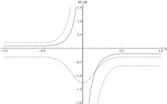
j ¼ Z X d2p dh2ðhðxÞÞhiðxÞhjðxÞdx: ð20Þ

Fig. 2depictsdU=dh¼dU=dM M0ðhÞfor a transonic flow through the nozzle shown inFig. 1. The density (solid) and total energy (dash-dotted) sensitivities are singular at the throat, while the mass flux (dashed) sensitivities are continuous.

3.3. Gradient and Hessian for the shock case

When shocks are present in the domain we takeX¼X_[Xþ_{such thatx}

sh¼X\Xþ. In this case, the objective function

(3)can be written as follows: J¼ Z Xp _{ðhðxÞÞdxþ}Z Xþp þ_{ðhðxÞÞdx;}

wherepþ_{ðhðxÞÞandpðhðxÞÞindicate the subsonic and supersonic pressure function to the right and to the left of the shock} respectively.

The functionp_ðx>x

shÞcan be interpreted as the extension of the supersonic pressure afterxsh, while the function

pþ_ðx<x

shÞas the extension of the subsonic pressure beforexsh. These two functions are continuous at the shock. Let us define

J ð

x

Þ ¼ Z x a p_{ðhðxÞÞdx and J}þ ð

x

Þ ¼ Z b x pþ_{ðhðxÞÞdx;}

whereX¼ ½a;b,a<xsh<b, anda<

x

<b. The integralsJð

x

ÞandJþð

x

Þare smooth functions of

x

for the pressure

min-imization problem. For the case of inverse design with a target pressure distribution that contains a shock, this argument does not always hold, as will be discussed in the next subsection.

The gradient is given by dJ d

a

i¼ Z X dp dh hiðxÞdxþ Z Xþ dpþ dhhiðxÞdx ðp þ_ðhðx shÞÞ pðhðxshÞÞÞ dxsh d

a

i : ð21Þ

The Hessian is obtained by taking the partial derivative with respect to

aj

of Eq.(21). When taking the derivative of the jump term we make use of the fact that the shock intensity does not change with the design variables,

pþ_ðhðx

shÞÞ pðhðxshÞÞ ¼const, although the shock location does move, therefore,

d2J d

a

id

a

j ¼ Z X d2p dh2 hiðxÞhjðxÞdxþ Z Xþ d2pþ dh2 hiðxÞhjðxÞdx ð22Þ dp þ dhðhðxshÞÞ dp dh ðhðxshÞÞ hiðxshÞ dxsh d

a

j ðpþ_ðhðx shÞÞ pðhðxshÞÞÞ d2xsh d

a

id

a

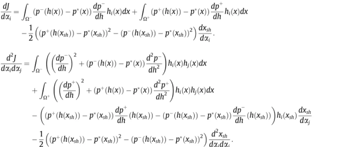
j :

3.4. The inverse design problem

Let us now consider the objective function (4). The above formulas for the gradient and Hessian hold with minor modifications: 1.0 0.5 0.5 1.0X 2.0 1.5 1.0 0.5 0.5 1.0 1.5 dU dh

Fig. 2.Sensitivity solution for transonic flow. The solid line represent the density sensitivity, the dashed is the mass flux sensitivity, and the dash-dotted is the total energy density sensitivity.

dJ d

a

i ¼ Z Xðp _{ðhðxÞÞ pðxÞÞ}dp dh hiðxÞdxþ Z Xþðp þ_{ðhðxÞÞ pðxÞÞ}dp þ dh hiðxÞdx 1 2 ðp þ_ðhðx shÞÞ pðxshÞÞ2 ðpðhðxshÞÞ pðxshÞÞ2 _dxsh d

a

i : ð23Þ d2J d

a

id

a

j ¼ Z X dp dh 2 þ_ðp_{ðhðxÞÞ pðxÞÞ}d 2 p dh2 ! hiðxÞhjðxÞdx þ Z Xþ dpþ dh 2 þ_ðpþ_{ðhðxÞÞ pðxÞÞ}d 2 pþ dh2 ! hiðxÞhjðxÞdx pþ_ðhðx shÞÞ pðxshÞ ð Þdp þ dh ðhðxshÞÞ ðp _ðhðx shÞÞ pðxshÞÞ dp dh ðhðxshÞÞ hiðxshÞ dxsh d

a

j 1 2 ðp þ_ðhðx shÞÞ pðxshÞÞ2 ðpðhðxshÞÞ pðxshÞÞ2 _d2 xsh d

a

id

a

j : ð24Þ

The target pressure distributionp_{is in principle arbitrary. In the case that it is discontinuous atx}

sh, then the functional

inte-grandsðp_{ðhðxÞÞ pðxÞÞ}2

andðpþ_{ðhðxÞÞ pðxÞÞ}2

contain a jump at the shock. Therefore the integrals Jð

x

Þ ¼ Z x a 1 2ðp _{ðhðxÞÞ pðxÞÞ}2 dx and Jþð

x

Þ ¼ Z b x 1 2ðp þ_{ðhðxÞÞ pðxÞÞ}2 dx;

have a discontinuous derivative at

x

¼xsh. As a result both the gradient and the Hessian do not exist at that point. An

exam-ple of such a situation is given in Section4.2. 4. Computational results using the direct method

The flow conditions for all the cases below arep0_{¼2,H¼4 at the inlet. For the cases with a shockp¼1:1 at the outlet.} The geometry is defined by X¼ ½1;1 and h0ðxÞ ¼2 for 1x<1=2, h0ðxÞ ¼1þsin2ð

p

xÞ for 1=26x61=2, and

h0ðxÞ ¼2 for 1=2<x61. With these conditions a shock is present in the flow field atxsh¼0:3941, corresponding to a

chan-nel height of 1:893.

The B-splines basis functions are uniformly distributed starting after the throat and in the diverging part of the nozzle. We denote byNthe number of collocation points in the interval½0:1;0:5. The support of the basis functions is compact,hiðxÞis

non-zero only between the collocation pointi2 andiþ2. This allows the study of the effect induced by localized geomet-rical perturbations on the flow.

4.1. Pressure minimization

We compute the condition number of the Hessian for the pressure minimization objective function(3)as a function of the number of design variables. We consider three cases: a subsonic flow, a transonic flow with supersonic exit, and a transonic shocked flow, seeFig. 3. In the subsonic casep¼1:98 at the outlet, whereas in the transonic case the nozzle is adapted. In the supersonic caseM¼3 at the inlet.

2.4 2.6 2.8 3.0 3.2 3.4 3.6 Log N 3 4 5 6 7 8 9 Log COND

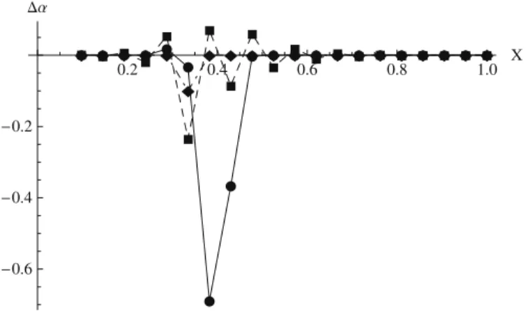
For the shocked case the condition number increases significantly as the number of design variables increases, whereas for the subsonic or the transonic cases it stays almost unchanged. In the presence of a shock, larger and larger numbers are obtained close to the Hessian diagonal as the number of design variables increases (seeFig. 5) resulting in a larger condition number. This behavior is due to the fact that the splines become more and more localized, steeper (non-differentiable at the limit), and therefore the large values around the diagonal at the shock location is a direct consequence of Eq.(18). For the shocked case, inFig. 4, we show the gradient as well as the gradient pre-multiplied by the inverse of the Hessian as a function of the corresponding B-spline collocation point. The gradient curve is proportional to the shape update (D

a

) in a steepest descent optimization method. On the other hand, the plot of the gradient pre-multiplied by the inverse of the Hessian in-verse represents the correction to a given shape in a Newton’s method. The two curves are strikingly different.

4.2. The inverse problem

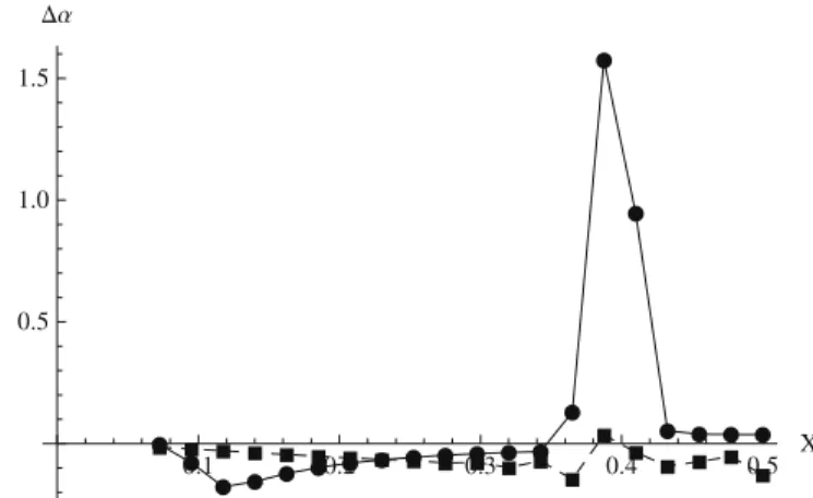
We calculate the Hessian for the inverse problem consisting in minimizing the objective function defined in Eq.(4). The minimum is given by the values of the design variables that were used to compute the target pressurep_{. In this case the} target pressure is that relative to the unperturbed geometryh0ðxÞ. Hence, in addition to what was shown for the previous case, we are able to show the plot of the error, i.e., the difference between the present value of the design variable and the value corresponding to the minimum.

The number of design variables considered isN¼20. The position of the shock can be perturbed by shape function num-ber 4, 5, and 6 (due to their collocation). Indeed, inFig. 5we can observe the presence of large values on the 4th, 5th and 6th columns. InFig. 6one can see that the inverse of the Hessian gives an appropriate correction to the gradient by shifting the curve’s peak to the left, the location of the only non-zero component of the error. In fact, we have only perturbed shape func-tion 6.

Finally, we study the case where the target pressure distributionp_{has a shock located at an identical location as the} shock of the pressure,p, for the current geometry. As discussed earlier the objective function integrand does not have con-tinuous prolongations from the left and from the right at the shock location, and hence the objective function is not differ-entiable with respect to those shape functions that can perturb the shock. We took 10 B-spline evenly distributed between

x¼0:05 andx¼1=2. The pressure at the exit ispex¼1:1 and the reference pressurepðxÞcorresponds to the unperturbed

nozzle shape. Under these conditions the shock is again located atxsh¼0:3941. InFig. 7we show the functional value when

a

2is varied between0.01 and 0.01. This design variable does not perturb the shock. In contrast,Fig. 8depicts the value of

0.1 0.2 0.3 0.4 0.5 X

0.5 1.0 1.5

Fig. 4.Pressure minimization problem. The solid line (circles) represents the gradient, the dashed (squares) represents the gradient pre-multiplied by the inverse of the Hessian.

Fig. 5.The Hessian for the inverse problem minimizing the integral ofðpp_Þ2

=2. Since the shape functions are local B-Splines, it is possible to relate the location of the shock wave with the 4th, 5th and 6th column of the Hessian having significantly larger values.

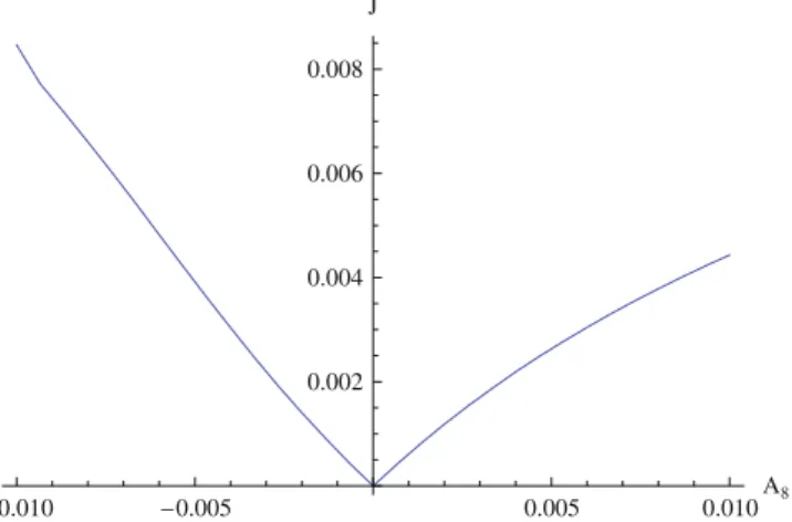
the functional when0:016

a

₈6_{0:01. The corresponding shape function does perturb the shock and when the two shocks} are aligned, for

a

8¼0, the functional is not differentiable. However, we speculate that in many practical computations the shock wave is smeared on a few grid points due to artificial or physical dissipation, and the issue of non-differentiability may not be observed.

5. Gradient and Hessian derivatives via adjoint equation approach

The direct method presented in Sections3 and 4was very useful to analyze the model problem at hand, but it is not prac-tical for industrial applications. In general we can not represent the solution as an explicit function of the geometry.

In this section we develop two methods that are viable for industrial applications, and that are based on the adjoint method.

5.1. The gradient via the adjoint method

The adjoint representation of the gradient is given by dJ d

a

i ¼ Z X vT_f idx; ð25Þ

where (recall thatL¼oR

oUandfi¼ oR oai) fi¼ ohi oxP d dxðhiFÞ : ð26Þ 0.2 0.4 0.6 0.8 1.0 X 0.6 0.4 0.2

Fig. 6.The solid line (circles) represents the gradient, dashed (squares) represents the gradient pre-multiplied by the inverse of the Hessian, and the dot-dashed (diamonds) represents the error. (Inverse problem with a design space consisting ofN¼20 design variables.)

0.005 0.005 0.010A2 0.00445 0.00446 0.00447 0.00448 J

Fig. 7.The objective function as a function of the single design variablea2. The objective function in this case is the inverse problem minimizing the integral ofðpp_Þ2

=2. The two shocks (in bothpandp_{) are aligned and the design variable does not perturb the shock location. The resulting curve is smooth}

The adjointvsatisfies the adjoint equation

L_v

¼op

oU; ð27Þ

where the application of the adjoint linearized operator is given explicitly by, Lv hATdv dx dh dxB T v: ð28Þ

5.2. Analytical derivation of the Hessian method I: Oð2Nþ1Þlinear solutions

The formal expression for the elementði;jÞof the Hessian is given by:

d2J d

a

id

a

j¼ Z X dv d

a

j T fiþvT dfi d

a

j " # dx: ð29Þ

We observe that applying the above formula to a case where shocks are present in the flow, the termfiis discontinuous at the

shock (Heaviside function) and the adjointvhas a log singularity at the throat but is continuous at the shock[5]. The termdfi

daj contains a delta function at the shock since the pressure,p, contains a Heaviside function.

The termfidepends on the design variables implicitly via the sensitivities. Its derivative with respect to

aj

is given by,

dfi d

a

j ¼ oL o

a

i dU d

a

j : ð30Þ

We take the derivative of the adjoint equation to obtain an equation for the adjoint sensitivity,dv=d

aj

:

Ldv d

a

j ¼ dL d

a

j vþdU d

a

j og oU; ð31Þ

wheregdenotes the right hand side (RHS) of the adjoint equation(27)given by

g¼op

oU: ð32Þ

Eq.(31)is similar to the adjoint equation but with a different right hand side. Denoting the RHS of Eq.(31)byGj, we have

Ldv

d

a

j

¼Gj: ð33Þ

In terms ofGjthe Hessian can be written as follows:

d2J d

a

id

a

j¼ Z X ½fiLGjdxþvT dfi d

a

j dx: ð34Þ 0.010 0.005 0.005 0.010A8 0.002 0.004 0.006 0.008 J

Fig. 8.The objective function as a function of a single design variablea8. The objective function in this case is the inverse problem minimizing the integral ofðpp_Þ2

=2. The two shocks (in bothpandp_{) are aligned and the design variable does perturb the shock location. The resulting curve is not smooth at the}

5.2.1. Derivation of the RHS of the adjoint sensitivity equation

The RHS of Eq.(31)Gj, can be represented as follows:

Gj¼ oL o

a

j vdU d

a

j oL oUvþ dU d

a

j o2p oU2; ð35Þ

where the adjoint operatorL_{has been differentiated by parts:} dL d

a

j ¼oL o

a

j þdU d

a

j oL oU: ð36Þ

Recall that the application of the adjoint operator on the derivative term is defined by, Ldv d

a

j hAT d dx dv d

a

j dh dxB Tdv d

a

j :

The cost of method I is the solution ofNsensitivity equations,Nadjoint sensitivity equations, and 1 additional adjoint equa-tion; all together 2Nþ1 linear equations. The termsLU;LaandJUU;JUaneed to be computed as well. In particular the term

containing the second order Jacobian tensor,JUU, may be difficult to implement using modern CFD codes.

5.3. Analytical derivation of the Hessian method II: OðNþ1Þlinear solutions

Our starting point is Eq.(29):

P

ði;jÞ d 2 J d

a

id

a

j¼ Z X dv d

a

j T fiþvT dfi d

a

j " # dx: ð37Þ 5.3.1. The term vT_ðdf i=d

aj

Þ

The derivative offiis computed explicitly from Eq.(26):

dfi d

a

j ¼ d d

a

j oR o

a

i ¼ oR 2 o

a

io

a

j o oU oR o

a

i dU d

a

j ¼ oL o

a

i dU d

a

j ; ð38Þ

where the second derivative with respect to

a

can be eliminated, since the residualRis linear in the design variables:

oR2

o

a

io

a

j ¼0:

5.3.2. The termðdv=d

aj

ÞTfi

The adjoint sensitivity term is derived by first considering the sensitivity equation: oR oU dU d

a

i þoR o

a

i ¼0:

In terms of the sensitivities we can write fi¼ oR o

a

i ¼LdU d

a

i : Therefore, Z X dv d

a

j T fidx¼ Z X dv d

a

j T LdU d

a

i dx:

Taking the adjoint of the right hand side integrand we get (using the identity,Ldv

daj¼Gj, andGjis given by Eq.(35)),

Z X dv d

a

j T fidx¼ Z X dU d

a

i T Ldv d

a

j dx¼ Z X dU d

a

i T o2p oU2 dU d

a

j oL oU dU d

a

j þoL o

a

j v ! dx ð39Þ

5.3.3. The Hessian in matrix form

Substituting relations(38) and (39)in(37)and rearranging terms, the Hessian can be represented in the following ma-trix–vector form:

P

ði;jÞ ¼ Z X dU dai 1 " #T o2_p oU2 T 0 0 0 " # v oL oU o L oaj oL oai 0 " # ( ) _dU daj 1 " # dx ð40Þ

The notationis introduced in order to clarify the application of the operators in the integrand on the sensitivities and ad-joint variables. It should be interpreted as follows:

voL oU dU d

a

j ¼oL oU dU d

a

j v voL o

a

j ¼oL o

a

j ðvÞ voL o

a

i dU d

a

j¼ v oL o

a

i dU d

a

j

where the parenthesisAðxÞdenotes the action of an operatorAonx, and the dotv xdenotes a dot product betweenvandx. The cost of method II consists of solvingNlinear sensitivity equations, and 1 additional adjoint equation; all together

Nþ1 linear equations. As in method I, the termsLU;LaandJUU;JUaneed to be computed as well.

Although method II seems to have an advantage over method I with regards to computational cost, we suspect that meth-od II is likely to be more delicate in practice for flows with shocks, based on the following argument. In the Hessian repre-sentation given by Eq.(40)the termsdU

dai, and

dU

dajcontain a delta function at the shock, while the terms

oL oaj, oL oaj, oL oUand o2_p oU2contain a Heaviside function. As mentioned before the adjoint variable,v, is continuous at the shock. The numerical implementation of Eq.(40)may be more delicate compared to that of Eq.(29)since some of the terms involve multiplication of delta func-tions at the shock. This is not the case for the Hessian representation of method I (recall the observation we have made fol-lowing Eq.(29)).

In the case of shocked flow for which the domain is not splitted to shockless subdomains, a more rigorous mathematical treatment is required to show that Eq.(40)can be interpreted in the sense of generalized functions, similar to the analysis done for the gradient in[11] and [12]. This is beyond the scope of this paper and is left for future investigation.

6. Numerical verification of the adjoint based methods for supersonic flow

We demonstrate the two methods on the model problem for shockless flow. In the quasi-one-dimensional approximation the domain can always be split into sub-regions where the solution is non-singular. We show here that the two methods yield the same results as the direct approach for a shockless case. The case considered is supersonic. The nozzle geometry is the same as that in previous sections. At the inlet the total pressure is given,p0_{¼2, as well as total enthalpyH¼4} and Mach numberM¼3. We consider a pressure minimization objective function overX¼ ½1;1. The shape functions are 10 B-splines with support evenly distributed in the interval½1=2;1=2. All the calculations are done using the Mathem-aticaÓ_{symbolic manipulation software.}

The Hessian is first determined by the direct method, Eq.(20), on the unperturbed nozzle, to obtain a reference point. The result is shown inFig. 9and later compared with results obtained using the adjoint based methods.

6.1. Adjoint method I: Oð2Nþ1Þlinear solutions

The Hessian representation by Eq.(29)requires the adjoint solution and its sensitivity derivatives. The adjoint is calcu-lated following the Green’s function method presented in[5]. In the following, the adjoint sensitivity derivatives are calcu-lated in a similar manner for supersonic flow condition.

We make use of the Lagrange identity for this case (j¼1;. . .;Nandk¼1;2;3):

ðGj;ukÞ ¼ dv d

a

j ;d~k : ð41Þ

Eq.(41)is a direct consequence of the adjoint definition:

Ldv d

a

j ;uk ¼ dv d

a

j ;Luk :

The left hand side of Eq.(41)is defined explicitly by, ðGj;ukÞ

Z 1 1

GjðxÞukðxÞdx: The right hand side is defined by,

dv d

a

j ;~dk Z 1 1 dv d

a

jð xÞdkðxÞdðxnÞdx; wheredðxÞdenotes the delta function atx.

The functionsukare assumed to be the solutions of the following linearized equation corresponding to three independent

right hand sidesdk:

Luk¼dkdðxnÞ: ð42Þ

In the supersonic casedkis given by the columns of the matrixDðxÞ, andDis defined by:

D ¼ 1 h

q

q=ð2HÞ h

q

q=p0 q 0 hð

q

q2_þpÞ=p0 H h

q

q=2 h

q

qH=p0_: 0 B @ 1 C A

The solutions of Eq.(42)are found in terms of the fundamental components (see[5])

1 h oU om H;p0 ;oU oH p0_;M ;oU op0 H;M 1 A: ð43Þ

For supersonic flow the Mach number,M, the enthalpy,H, and the total pressure,p0_{, are fixed at the inlet and there are no} boundary conditions at the outlet, resulting in

u1ðx;nÞ ¼ HðxnÞh1ðxÞo U omðxÞ_H;p0 u2ðx;nÞ ¼ HðxnÞ_ooUHðxÞp0_;M u3ðx;nÞ ¼ HðxnÞ_oo_pU0ðxÞ H;M;

whereHðxÞis the Heaviside function ofx. Each of the above three partial derivatives,(43), has to be evaluated for the three fundamental variables,U¼ ð

q

;

q

q;

q

EÞT.

The following matrix contains the key information required:

v

¼ 1 h oq omH;p0 oq oHp0;M oq op0 H;M 1 h om oHp0_{;M o}o_pm0 H;M 1 h oqE omH;p0 oqE oH p0_;M oqE op0 H;M: 2 6 6 6 6 6 4 3 7 7 7 7 7 5 ð44Þ

In terms of

v

the solutionsukcan be written as follows:

U ¼

v

A;

whereukform the columns of the matrixU, and where the columns of the matrixAare the three coefficient vectors

A ¼ HðxnÞ 0 0 0 HðxnÞ 0 0 0 HðxnÞ 2 6 4 3 7 5: ð45Þ

In terms of the above definitions, the adjoint sensitivity can be written in matrix notation as follows: dv d

a

m ðnÞ ¼ D1_ð nÞ Z 1 n GmðxÞ

v

ðxÞdx : ð46Þ

The results are presented inFig. 10. The numerical results for the Hessian, as computed by method I, coincide with the ref-erence solution, computed by the direct method, up to a numerical error. Let P be the Hessian, we have kPdirect Pmethod Ik=kPdirectk ¼1:5104. The source of numerical errors is primarily the numerical integration procedure, that is

6.2. Adjoint method II: OðNþ1Þlinear solutions

The Hessian representation by Eq.(40)does not require the adjoint sensitivity derivatives. In that sense method II is sim-pler to implement, it requires only the sensitivities and adjoint solutions. The result is demonstrated inFig. 11. In this case the numerical results have a smaller numerical integration error compared with method I: kPdirectPmethod IIk= kPdirectk ¼2:4106. Method I is less accurate since there is one more integration involved to compute the adjoint

sensitiv-ities, as opposed to method II where we integrate only once to compute the adjoint variables. This result indicates that in practice method I will require a tighter convergence tolerance than method II in order to achieve a similar accuracy. 7. Discussion

Industrial aerodynamic optimization problems are usually defined by hundreds of design variables and millions of state variables. The state-of-the-art practice is to use the adjoint method to compute the gradient, and quasi-Newton method to accelerate the convergence. Quasi-Newton approximates the Hessian (or its inverse) by a low rank update method taking the identity matrix to be the initial guess. That choice corresponds to having the gradient as the initial search direction in the optimization process.Fig. 6demonstrates how the gradient can serve as a poor search direction; the solid line (circles) rep-resents the gradient and the dot-dashed line (diamonds) reprep-resents the error. The gradient is both quantitatively and qual-itatively pointing in the wrong direction. For practical industrial aerodynamic optimization problems only a few iterations can be afforded, resulting in poor convergence. Therefore, we think that direct approximation of the Hessian is essential to achieve convergence in a relatively small number of iterations. Such an approximation can serve as the initial guess for a quasi-Newton method.

In this work we compute the Hessian analytically for an optimal shape design problem governed by the quasi-one-dimen-sional Euler equations, modeling inviscid flow in a channel. For that ideal model problem we can study the Hessian directly by representing the flow, sensitivity, and adjoint solutions as explicit functions of the design variables. That allows us to ex-plore the question of Hessian existence in aerodynamic optimization problems under transonic flow with shocks. The Hes-sian exists in the strong sense if the objective function is twice differentiable at every design point. Fig. 8serves as an example to the lack of smoothness that may occur in such problems. The objective function as a function of one of the design variables (

a

8) is not smooth at

a

8¼0, thus both the gradient and the Hessian do not exist at that point. We think that more research is required to further understand the existence of the gradient and Hessian in the presence of shocks, particularly at the discrete level where the choice of numerical scheme may make a difference.

We also propose two formulations to approximate the Hessian that can be applied to general problems for which the di-rect approach is not practical. These formulations are based on the adjoint and sensitivity solutions. The first method is more expensive. It requires solving the adjoint sensitivity equations in addition to the standard sensitivity equations and adjoint equation (Oð2Nþ1Þlinear solutions), while the second method requires only the sensitivity and adjoint equations (OðNþ1Þ

linear solutions). In practice the Hessian is used to obtain an improved search direction by preconditioning the gradient and therefore only an approximated Hessian is required. The computational effort can be greatly reduced by a number of ways,

Fig. 10.Hessian by the adjoint method I for supersonic flow condition (Oð2Nþ1Þlinear solutions).

for example by converging the sensitivity equations only to a low tolerance value. Also, the sensitivity equations system is easily parallizable as it consists of a single operator with many right hand sides.

The preliminary analysis presented in this paper suggests that the first method, although more expansive, may be more stable, since the second method involves multiplications of delta functions (d2) at the shock location suggesting large num-bers in the numerical computation (see discussion at the end of Section5). We demonstrate the application of the proposed two adjoint based methods on the model problem for supersonic flow. More research is required to better understand, from a numerical analysis view point, method I and method II to compute the Hessian. This is left for future study.

References

[1] A. Jameson, Aerodynamic design via control theory, ICASE report NO. 88-64, November, Journal of Scientific Computing 3 (1988) 233–260. [2] F. Beux, A. Dervieux, Exact-gradient shape optimization of a 2-D Euler flow, Finite Elements in Analysis and Design 12 (1992) 281–302.

[3] P.D. Frank, G.R. Shubin, A comparison of optimization-based approaches for a model computational aerodynamics design problem, Journal of Computational Physics 98 (1992) 74–89.

[4] A. Iollo, M.D. Salas, Contribution to the optimal shape design of two-dimensional internal flows with embedded shocks, Journal of Computational Physics 125 (1996) 124–134.

[5] M. Giles, N. Pierce, Analytic adjoint solutions for the quasi-1D Euler equations, Journal of Fluid Mechanics 426 (2001) 327–345. [6] B. Mohammadi, O. Pironneau, Shape optimization in fluid mechanics, Annual Review of Fluid Mechanics. 36 (2004) 255–279.

[7] E. Arian, S. Ta’asan, Analysis of the Hessian for aerodynamic shape optimization: inviscid flow, Computers and Fluids 28 (1999) 853–877. [8] E. Arian, V. Vatsa, A preconditioning method for shape optimization governed by the Euler equations, International Journal of Computational Fluid

Dynamics 12 (1999) 17–27.

[9] L. Sherman, A. Taylor III, L. Green, P. Newman, First- and second-order aerodynamic sensitivity derivatives via automatic differentiation with incremental iterative methods, Journal of Computational Physics 129 (1996) 307–331.

[10] D. Ghate, M. Giles, Efficient Hessian calculation using automatic differentiation, in: AIAA Paper 2007-4059, 25th AIAA Applied Aerodynamics Conference 25–28 June 2007, Miami, FL.

[11] C. Bardos, O. Pironneau, A formalism for the differentiation of conservation laws, Comptes Rendus Mathematique 335 (2002) 839–845. [12] C. Bardos, O. Pironneau, Data assimilation for conservation laws, Methods Applied Analysis 12 (2005) 103–134.