Characterisation studies on the optics of the prototype fluorescence telescope FAMOUS

Characterisation studies

on the optics of the prototype

fluorescence telescope

FAMOUS

von

Hans Michael Eichler

Masterarbeit in Physik

vorgelegt der

Fakultät für Mathematik, Informatik und Naturwissenschaften

der Rheinisch-Westfälischen Technischen Hochschule Aachen

im März 2014

angefertigt im

III. Physikalischen Institut A

bei

Erstgutachter und Betreuer Prof. Dr. Thomas Hebbeker III. Physikalisches Institut A RWTH Aachen University

Zweitgutachter

Prof. Dr. Christopher Wiebusch III. Physikalisches Institut B RWTH Aachen University

Abstract

In this thesis, the Fresnel lens of the prototype fluorescence telescope FAMOUS, which is built at the III. Physikalisches Institut of the RWTH Aachen, is characterised. Due to the usage of silicon photomultipliers as active detector component, an adequate optical performance is required. The optical performance and transmittance of the used Fresnel lens and the qualification for the operation in the fluorescence telescope FAMOUS is examined in several series of measurements and simulations.

Zusammenfassung

In dieser Arbeit wird die Fresnel-Linse des Prototyp-Fluoreszenz-Teleskops FAMOUS charakterisiert, welches am III. Physikalischen Institut der RWTH Aachen gebaut wird. Durch die Verwendung von Silizium-Photomultipliern als aktive Detektorkomponente werden besondere Anforderungen an die Optik des Teleskops gestellt. In verschiedenen Messreihen und Simulationen wird untersucht, ob die Abbildungsqualität und die Transmission der verwendeten Fresnel-Linse für die Verwendung in diesem Fluoreszenz-Teleskop geeignet ist.

Contents

1. Introduction

2. Cosmic rays

2.1 Energy spectrum

2.2 Sources of cosmic rays

2.3 Extensive air showers

3. Fluorescence light detection

3.1 Fluorescence yield

3.2 The Pierre Auger fluorescence detector

3.3 FAMOUS

4. Introduction to lenses and Fresnel lenses

4.1 Conventional lenses

4.1.1 Point spread function

4.1.2 Diffraction limit

4.1.3 Aberrational effects

4.2 Fresnel lens

4.2.1 Basic concept

4.2.2 Manufacturing

4.2.3 Diffraction of a Fresnel lens

4.2.4 Transmittance

4.2.5 Focal point of a Fresnel lens

5. Measurement setup

5.1 Point light source

5.2 Dark room

5.3 Light sensor

5.4 Test bench

6. Raytracing simulation

6.1 Fresnel lens groove profile

6.2 Wave characteristics of photons

1

3

. . . 4

. . . 6

. . . 7

11

. . . 11

. . . 14

. . . 16

21

. . . 21

. . . 23

. . . 25

. . . 28

. . . 31

. . . 31

. . . 32

. . . 33

. . . 35

. . . 36

37

. . . 37

. . . 41

. . . 42

. . . 46

49

. . . 49

. . . 55

7. Analysis framework

7.1 Brightness measurement with a camera CMOS chip

7.2 Bayer pattern

7.3 Dynamic range

7.3.1 High dynamic range feature

7.4 Background and noise subtraction

7.4.1 Offset correction

7.5 Image compilation

8. Aberration radius and best focus

8.1 Measurement of the aberration radius

8.2 Results of the measurement

8.3 Results of the simulation

8.4 Alignment test and systematical uncertainty

9. Transmittance

9.1 Experimental setup and procedure of measurement

9.2 Measured and simulated results

10. Summary and outlook

References

Acknowledgements - Danksagungen

57

. . . 57

. . . 59

. . . 60

. . . 61

. . . 64

. . . 65

. . . 67

71

. . . 71

. . . 73

. . . 75

. . . 77

83

. . . 83

. . . 87

89

91

95

List of figures

1.1 Logo of FAMOUS

2.1 All-particle cosmic ray energy spectrum

2.2 Hillas plot of known astrophysical sources for cosmic rays

2.3 Schematic of an air shower formation in the atmosphere

2.4 Components of the photon attenuation coefficient

2.5 Energy deposit as function of the slant depth X

3.1 Molecular levels of nitrogen N

₂

and N

₂+

3.2 Air fluorescence spectrum as function of the photon wavelength

3.3 Map of the Pierre Auger Observatory

3.4 Schematic of an Auger fluorescence telescope

3.5 Picture of the seven pixel prototype of FAMOUS

3.6 Refractive optical design of FAMOUS

3.7 Picture of the seven-pixel-focal-plane of FAMOUS SEVEN

3.8 Simulated trigger probability of FAMOUS

4.1 Different types of lenses

4.2 Construction of a lens surface with cylindrical coordinates

4.3 Conic sections

4.4 Image formation of a refractive optical system

4.5 Influence of the point spread function

4.6 Sketch visualising the Abbe diffraction limit

4.7 Airy pattern on the image plane (distribution)

4.8 Airy pattern on the image plane (principle)

4.9 Spherical and aberrated wavefronts

4.10 Geometrical construction of comatic aberration

4.11 Geometrical construction of astigmatism

4.12 Petzval field curvature

4.13 Basic construction principle of a Fresnel lens

4.14 Cross section of a groove with relatively high slope angle

4.15 Radial intensity distribution of the diffraction pattern for a Fresnel lens

4.16 Encircled energy of the diffraction pattern of the Fresnel lens

4.17 Measured thickness of the Fresnel lens of FAMOUS

4.18 Simulated R90 of a Fresnel lens as a function of its focal number N

. . . 2

. . . 4

. . . 7

. . . 8

. . . 9

. . . 10

. . . 12

. . . 12

. . . 14

. . . 15

. . . 16

. . . 17

. . . 18

. . . 19

. . . 22

. . . 22

. . . 23

. . . 24

. . . 25

. . . 25

. . . 26

. . . 27

. . . 28

. . . 29

. . . 30

. . . 30

. . . 31

. . . 32

. . 34

. . . 34

. . . 35

. . . 36

5.1 Infinitely distant and near illumination of the Fresnel lens

5.2 The light source

5.3 Radiation pattern of the used UV LED

5.4 Spectrum of the used UV LED

5.5 Simulated best focus aberration radius as a function of the wavelength

5.6 Aberration radius with individual and common background image

5.7 Top view of the experimental setup

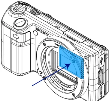
5.8 Top view of the Sony Nex-5

5.9 Sketch of the Sony Nex-5 without lens

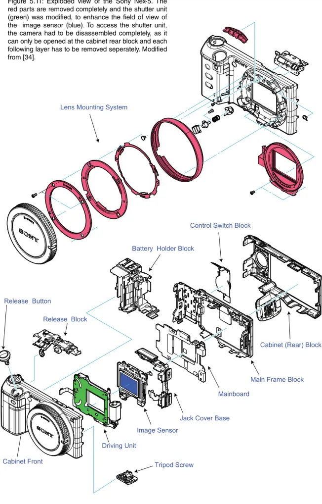
5.10 Picture of the modified Sony Nex-5

5.11 Exploded view of the Sony Nex-5

5.12 Camera mounted on a height-adjustable post

5.13 Top view on the test bench for two inclination settings

5.14 Photo of the test bench with close-up of angle scale

6.1 Top view of the simulation layout for two different incidence angles

6.2 Aberration radius for different draft angles and peak rounding radii

6.3 Dynamic draft angle

ψ

6.4 Transmittance for different draft angles and peak rounding radii

6.5 Cross section of a groove of the simulated Fresnel lens

6.6 Solution for inner grooves of the simulated lens

6.7 Microscopy picture of a slightly tilted Fresnel lens

6.8 Simulated aberration radius with and without diffraction

7.1 Linear encoded and gamma encoded brightness gradient

7.2 Brightness levels of pictures with different exposure times

7.3 Construction of a Bayer filter mosaic

7.4 The dynamic range of a scene

7.5 Construction of high dynamic range image

7.6 Profile of long exposure and short exposure image

7.7 Profile of HDR image of FAMOUS focal region

7.8 Row of pixels after background image subtraction

7.9 Row of pixels of figure 7.8 after offset correction

7.10 Influence of offset correction

7.11 Schematic of image compilation

7.12 Measured best focus PSF for an incidence angle θ = 10°

7.13 Simulated best focus PSF for an incidence angle θ = 10°

7.14 Schematic of the most important steps of image processing

. . . 38

. . . 39

. . . 39

. . . 40

. . . 40

. . . . 41

. . . 42

. . . 43

. . . 44

. . . 44

. . . 45

. . . 46

. . . 47

. . . 48

. . . 50

. . . . 51

. . . 51

. . . 52

. . . 53

. . . 54

. . . 54

. . . 55

. . . 58

. . . 58

. . . 59

. . . 61

. . . 62

. . . 63

. . . 63

. . . 65

. . . 66

. . . 66

. . . 67

. . . 68

. . . 68

. . . 69

8.1 Top view on the curved image plane of the Fresnel lens

8.2 Best focus point spread function for an incidence angle θ = 0°

8.3 Measured aberration radius as a function of distance to the Fresnel lens

8.4 Simulated aberration radius as a function of distance to the Fresnel lens

8.5 Comparison of measured and simulated best focus aberration radius

8.6 Measured aberration radius for angles of incidence θ = 4° and θ = -4°

8.7 Measured focal plane of the Fresnel lens

8.8 X-position of maximum & center of gravity of PSF for conventional lens

8.9 X-position of maximum & center of gravity of PSF for Fresnel lens

8.10 Measured best focus point spread function of a conventional lens

8.11 Point spread function divided into a vertical and a horizontal part

8.12 Aberration radius for vertical and horizontal parts

9.1 Aluminium plate with a milled window

9.2 Top view of the experimental setup for the measurement of the transmittance

9.3 Captured image of the light passing through the window

9.4 Captured light after passing the window and the center of the Fresnel lens

9.5 Measured transmittance of the Fresnel lens

. . . 70

. . . 72

. . 72

. . 73

. . . 74

. . . 75

. . . 76

. . 77

. . . . 77

. . . 78

. . . 80

. . . 80

. . . 82

. . 83

. . . 84

. 84

. . . 85

1 Introduction

The sky and its visible phenomena hold a strong fascination for everyone. As could have been expected, the most interesting facets - especially for scientific research - are not directly visible for the human eye.

This is also the case for cosmic rays, particles having incredibly high energies up to 1020 _{eV which predominantly originate outside of our solar system, ceaselessly striking} the atmosphere of the Earth. The sources and acceleration mechanisms of these particles are mostly unknown. Due to their low flux, which is below one per year and square-kilometer for energies above 1019 _{eV, the observation and corresponding studies} are challenging. To collect as much statistics as possible in a certain period of time, which is - among others - the aim of the Pierre Auger Observatory, the only approach is the construction of detectors covering as much surface as possible.

As those incoming particles - also called primaries - enter the atmosphere, cascades of secondary particles are induced like in a calorimeter, containing a hadronic, muonic and electromagnetic component. Besides emitting Cherenkov radiation in flight direction, the contained electrons and positrons also excite nitrogen molecules which, as a consequence, emit fluorescence photons in the UV range isotropically distributed. Instead of observing the primary directly, this calorimetric measurement is viable at far distance, making it possible to scan a large area with only few detectors.

However, as inherent to the described principle, the fluorescence signal is weak and a detection is possible only in clear dark nights. To still allow a measurement of such low light fluxes, the use of photomultiplier tubes is quite popular because of their high photon detection sensitivity, in conjunction with a large focusing mirror.

As an alternative to this traditional setup, a relatively new kind of semiconductor light sensor is used as the active detector component of the prototype fluorescence telescope FAMOUS (figure 1.1). The acronym, standing for First Auger MPPC camera for the Obser-vation of Ultra high energy cosmic ray air Showers, emphasizes the usage of so-called Multi Pixel Photon Counters - also known as silicon photomultipliers (SiPMs) which are built from a Geiger-mode avalanche photodiode array. As the name suggests, these devices are sensitive enough to detect single photons and thus are suitable to detect fluorescence radiation. In comparison to photomultiplier tubes, SiPMs operate at much lower voltage and promise a higher photon detection efficiency in the future.

For the prototype FAMOUS, a refractive telescope design was chosen using a Fresnel lens of roughly half a meter diameter. On that scale, Fresnel lenses have certain advantages in comparison to bulky lenses if image quality is of secondary importance. As a Fresnel lens is significantly thinner than its bulky counterpart, the transmittance of light in the ultraviolet regime is much higher, which is important since the characteristic spectrum of fluorescence radiation reaches from 280 nm to 420 nm. On top of that, a more compact and lightweight construction is possible.

In this thesis, the optics of the fluorescence telescope FAMOUS is characterised with special regard to the properties of the Fresnel lens, including the form of the focal point, various aberrational effects like spherical and coma aberration, distortion, curvature of field and the transmittance. Therefore, the listed effects are measured for the Fresnel lens of FAMOUS and for a conventional lens of smaller diameter to understand the influence of the experimental setup. Furthermore, the results are compared to a simulation of the setup.

As a result of this analysis, the systematic effects and influence of the Fresnel lens on the detector response of FAMOUS as well as the cooperation of the lens and the SiPM camera pixels can be better understood and quantised. The results will help to compute the uncertainties for the detected fluorescence signal.

Figure 1.1: Logo of FAMOUS: “First Auger Multi pixel photon counter camera for the Observation of Ultra-high-energy cosmic ray air Showers”

2 Cosmic rays

When Viktor Hess launched his balloon-experiments in 1912, he opened a new window to the cosmos and hence gave birth to the modern field of astroparticle physics. His measurements were the first to indicate the existence of cosmic rays [2]. To date the explanation of the ionisation of air was based on radioactive material in the Earth. As this assumption is partially true, the ionisation rate descends on the first thousand meters of altitude. However, beyond that height, the intensity increases again, revealing a second component which seems to have an extraterrestrial origin.

Ongoing experiments were able to uncover the secrets behind these observations. With the help of new technologies, a maximum of ionisation was found to be at 15 km height. In the hope to proof that the cosmic rays are high energetic gamma rays, producing secondary compton electrons, Walter Bothe and Werner Kolhörster found a majority of charged particles that could penetrate 4.1 cm of gold, which was an inconsistent observation to the assumed theory [3]. With other experiments measuring coincidences at large lateral distances, it could be concluded that the detected radiation consists of charged particles which are produced by primary cosmic rays.

Today, these secondary particles are well understood and known as extensive air showers. The measurement of extensive air showers is an important part of modern - indirect - detection methods for cosmic rays (CR). The majority of questions which are still unanswered today, address the ultra high energy cosmic rays which have energies higher than 1018 _{eV. Due to the very} low flux, neither origin nor composition of these particles is known today as they arrive isotropically at our atmosphere. By contrast, the composition of their lower energy pendants is well measured and summarised in table 2.1 [4]. Z Element F 1 H 540 2 He 26 3-5 Li-B 0.40 6-8 C-O 2.20 9-10 F-Ne 0.30 11-12 Na-Mg 0.22 13-14 Al-Si 0.19 15-16 P-S 0.03 17-18 Cl-Ar 0.01 19-20 K-Ca 0.02 21-25 Sc-Mn 0.05 26-28 Fe-Ni 0.12 Table 2.1: Relative abundances F of CR nuclei with E = 10.6 GeV

2.1 Energy Spectrum

One extensively studied property of cosmic rays is their energy spectrum. It shows the flux density as a function of energy. Summarising the results of many experiments, the spectrum is now measured over 31 orders of magnitude in flux and 11 orders in energy. The flux, getting steeper with energy, generally follows a power law [4]

with a spectral index γ = 2.7 to γ = 3.3. Here,

n

is the number of incoming cosmic rays with energy E per time

t

, solid angle Ω and area A. This provides a first indication for

nonthermal accelerating sources.

Figure 2.1: The all-particle cosmic ray spectrum as a function of the energy E compiled from different air

shower measurements. The flux is multiplied by a factor E2.6 _{to make the features known as knee, second}

knee and ankle better visible. The spectrum follows a power law with changing spectral index γ from 2.7

to 3.1. Above an energy of 1020 _{eV, the spectrum is cut off by yet undetermined reason. Taken from [2].}

[eV]

E

]

-1

sr

-1

s

-2

m

1.6

[GeV

F(E)

2.6

E

Grigorov JACEE MGU Tien-Shan Tibet07 Akeno CASA-MIA HEGRA Fly’s Eye Kascade Kascade Grande 2011 AGASA HiRes 1 HiRes 2 Telescope Array 2011 Auger 2011

Knee

Ankle

2nd Knee

10

13

10

14

10

15

10

16

10

17

10

18

10

19

10

20

1

10

10

2

10

3

10

4 (1)

As marked in figure 2.1, the spectral index changes at different characteristic energies. The first feature to be identified at an energy of 1015.5 _{eV is known as knee. Here, the} spectrum gets even steeper with energy. The spectral index changes from γ = 2.7 to γ = 3.1. At a slightly higher energy of 4 · 1017 _{eV a second downturn to γ = 3.3 was} observed later, thus it was called the second knee. In the ultra high energy regime, another feature was observed at 4 · 1018 _{eV. As the change in spectral index is now} negative, switching to γ = 2.6, this characteristic point is called ankle. At an energy of about 1020 _{eV, the spectrum cuts off.}

The explanation for the observed structures is accompanied by the understanding of the acceleration and propagation mechanisms of cosmic rays which are presently debated [5]. In one of the favourite approaches, the knee is explained as a consequence of the upper limit of acceleration by galactic sources, whereas a second component for extragalactic sources, which should be harder, but less intense, would dominate the spectrum from the ankle to the highest energies [5]. Another explanation for the knee includes the magnetic field of our galaxy: The Larmor radius

describes the circular motion of a particle with charge Z and an energy E in presence of a magnetic field B. Evaluating the latter equation for energies above E=1018 eV (=103 _{PeV) and magnetic field strength B of around 3 µG shows that the larmor radius} for protons exceeds the thickness of the galactic disk of around 0.1 kpc1 _{at that point.} As a consequence, protons with such a high energy are not bound to the galaxy and will escape after a certain path length. This results in a characteristic cut-off energy for protons as well as for all other elements of the periodic table, which were all found to be part of the composition of cosmic rays, at low energies partially reflecting the element composition of the solar system. For elements with higher charge Z, the cut-off appears at higher energies. As a result, the knee might represent the cut-off for protons, followed by subsequent cut-offs for the other elements, which form the relatively flat part of the all-particle spectrum above the knee. The second knee is assumed to be formed by the cut-off of ultra heavy nuclei which represents the upper energy limit of the galactic component [3].

As mentioned before, the spectrum decreases significantly at an energy of approximately 1020 _{eV. Due to the flux, which drops below one particle per century and} square-kilometer, only 47 events of energies higher than E = 3 · 1019 eV have been observed by the Pierre Auger Observatory in total [6]. Thus, it is very difficult to verify the existing theories concerning the cut-off of the all particle spectrum. The simplest explanation for this is the lack of sources capable to accelerate particles to higher energies. Besides this assumption, the Greisen-Zatsepin-Kuzmin (GZK) limit also predicts a cut-off of the spectrum above 6 · 1019 _{eV due to significant energy losses during propagation, caused} by interactions of protons with photons of the cosmic microwave background [5].

2.2 Sources of cosmic rays

In the previous chapter, the energy spectrum was described to follow a power law. This provides first information about the acceleration mechanisms to accelerate particles to high energies. One of the mainly accepted mechanisms by which particles gain nonthermal energies is called Fermi acceleration [7]. The main idea of this theory is multiple elastic scattering of energetic particles off magnetic turbulences, allowing them to pass many acceleration cycles in shock fronts. In each cycle, the particle energy gain is proportional to the characteristic velocity β_s = v/c of the shock front. The maximum energy of a particle E_max with charge Z then depends on the size R and the magnetic field strength B of the source:

In the Hillas plot (cf. figure 2.2), the maximum achievable energy of known astrophysical objects are presented as a function of size and magnetic field strength. In addition, the diagonal lines denote a limit for sources to accelerate protons to 1020 _{eV. Most of} the sources, except for neutron stars and possibly gamma ray bursts (GRB), seem too weak to accelerate particles to the highest energies, which have already been observed. However, the Hillas plot has to be regarded with caution since large uncertainties are involved, which are not plotted.

Apart from the acceleration of particles, which is known as the bottom-up model, another scenario is popularly proposed for the origin of cosmic rays, known as top-down model. It uses possible physics beyond the standard model of particle physics to describe the origin of ultra high energy cosmic rays: The decay of very high mass relics from the early universe, e.g. particles which could have been produced after the end of inflation, can decay into secondaries with energies even up to 1025 _{eV [8].}

According to the GZK theory, particles reaching us with energies above 1020 _{eV should} originate from sources closer than 100 Mpc [7]. As the eligible sources within this radius are limited, the isotropic arrival directions of particles in the energy regime which is measured is another property which is not yet understood. To develop a better understanding of the origin of ultra-high energy cosmic rays, large surface detectors like the Pierre Auger Observatory were built, to gather more statistics on using indirect detection principles: the study of extensive air showers.

Figure 2.2: The Hillas plot illustrates known astrophysical sources for cosmic rays as a function of magnetic field strength and size of the source, to accelerate particles to the highest observed energies. The diagonal lines mark the combination of size and field strength for a source being

capable of accelerating protons to 1020 _{eV with two characteristic velocitiesβ}

s. Adapted from [7].

2.3 Extensive Air Showers

When a cosmic ray enters the atmosphere of the Earth, its energy is transferred to many secondary particles, which are created due to decays and inelastic scattering with molecules of the air [7]. As a result, an avalanche of ionised particles and electro-magnetic radiation evolves through the atmosphere. Despite the fact that the formation of such cascades relies on stochastic processes, they can be well described by suitable models. The analysis of extensive air showers allows to conclude on properties of the primary cosmic rays.

As illustrated in figure 2.3, the composition of an air shower for a primary particle can be separated into three components: a hadronic, an electromagnetic and a muonic. The hadronic cascade is the starting point for the two other components, as the continuous interactions also generate neutral pions, which decay almost instantly into two photons, repeatedly generating the electromagnetic component of the shower while the muonic component arises from the decay of charged pions or kaons. The dominant decay mechanisms are also summarised in figure 2.3.

Active Galactic Nuclei

E

_max

~

= 1

= 1 / 300

Neutron stars

GRB ?

White

dwarfs

LHC

Interplanetary

space

SNR

Galactic

Disk

Halo

Radio

galaxy

jets

Galactic

cluster

IGM

10 eV Pr

otonen

20

Magnetic field B / Gauss

10

-6

1

10

6

10

12

Size R

1km

10

6

km

1pc

1kpc 1Mpc

1AE

β

β

β

s s s

· Z · R · B

π

µ

γ

K

n

p

v

π

0

γ

e

+

e

-γ

γ

γ

γ

p

n

π

±

π

+

µ

+

ν

_µ

n

p

K

-π

-π

0

µ

-ν

_µ

π

-ν

_µ

µ

-n

K

±

π

+

µ

+

ν

_µ

ν

_µ

e

-e

+

e

-e

+

e

-e

-e

+

e

+

ν

_e

e

+

π

±

K

±

p

Atmospheric nucleus Primary cosmic ray Slant depth ~ 1000 g cm -2 Electromagnetic

π

0

→

γ

+

γ

,,

γ

→

e

+

+

e

-,

e

±

→

e

±

+

γ

Hadronic p

+

A

→

p

+

X

+

π

±,0

+

_K±,0

+ ...

A = Atmospheric nucleus X = Fragmented nucleus Muonic

π

±

→

ν

_µ

+

µ

± K±

→

ν

µ

+

µ

±

Figure 2.3: Schematic of an air shower formation in the atmosphere. The primary cosmic ray collides with an air molecule which generates unstable hadrons like pions and kaons as well as protons and neutrons. Starting from the decay of these neutral and charged hadrons, the electromagnetic and muonic components of the air shower are generated. The dominant interaction and decay processes are summarised on the bottom of the picture. Background picture adapted from [1].

The general structure of an extensive air shower depends on the incident particle. First, an electromagnetic shower, which can be induced by electrons, positrons or photons, will be discussed. A simple, but effective model to describe the development of an electromag-netic cascade was presented by Heitler [7]. The main idea of the Heitler model is that each electromagnetic particle will undergo two-body splitting after a mean interaction length λ_int as long as the particle energy drops below a critical energy E_C (figure 2.4), from which energy loss due to Compton scattering for photons and ionisation for charged particles become more dominant than pair production. In a first approximation, the energy of the mother particle E₀ is divided equally among the daughter particles with energy E₁:

For high energetic electrons, the primary interaction process is bremsstrahlung, whereas photons convert into an electron positron pair. With this approach, the electromagnetic shower can be divided into segments with distances of

λ

int, every segment “n” containing N = 2n particles with a resulting energy _E

n for each of the particles:

As mentioned before, this process of duplication stops when the energy of the particles drops below the critical characteristic energy E_C (figure 2.4). From this point, the number of particles decreases again due to absorption processes. This allows the calculation of the stage n_max, that contains most particles N_max :

Including the interaction length in air for the described processes, the slant depth X of the shower maximum can be determined, which describes the amount of matter that

Figure 2.4: Components of the photon attenuation coefficient in 1/gcm-2 _{in air as function of the energy.}

At the critical energy E_C pair production becomes the most dominant effect. Adapted from [9].

Energy in MeV

Attenuation in 1 / (cm

-2

g)

10-2 ₁₀-1 ₁₀0 ₁₀1 ₁₀2 101 100 10-1 10-2 10-3

Critical energy E

_C

Rayleigh scat.Photo. absorp.

Photon mass attenuation coefficients in air

(4)

(5)

has to be passed by integrating the density of the atmosphere ρ from a given altitude h to the top of the atmosphere using ρ₀ =1.35kg m-3 _{and h}

0 = 7.25km:

One of the most popular models to describe these showers is known as the Gaisser Hillas function [10]:

It is used to parameterise the longitudinal particle density of extensive air showers with four parameters: X_max is the atmospheric depth of the shower maximum in cm-2 _{g, N}

max the maximum number of shower particles and

λ

as well as X₀ are fit shape parameters, which have no direct physical meaning. As shown in figure 2.5, the parameterisation describes the longitudinal profile of a measured shower very well. In this plot, the deposited energy of the shower particles as function of the slant depth, dE/dX, is presented, which is related to the number of shower particles per slant depth. The parameters, determined with the Gaisser Hillas fit, bear information about the energy and mass of the primary particle, thus they can also be used to study the chemical composition of cosmic rays.

To obtain the necessary information on the longitudinal shower profile, the fluorescence light, which is emitted by nitrogen molecules in cause of the ionising particles of the air shower, can be recorded by imaging telescopes. This fluorescence detection principle is discussed in the next chapter.

Figure 2.5: Energy deposit as a function of the slant depth X, reconstructed from the light of one air shower observed by a fluorescence telescope of the Pierre Auger Observatory. The red line denotes the Gaisser Hillas function fitted to the data. Adapted from [11].

Slant depth in cm-2 _g dE /dX in PeV / (cm -2 g) 0 10 20 30 40 50 / Ndf = 42.45 / 44 2 χ 200 400 600 800 1000 1200 1400 1600 X_max (7) (8)

3 Fluorescence light

detection

The measurement of extensive air showers by detecting the emitted fluorescence light is an established procedure. With the functionality of a calorimeter, the atmosphere of the earth becomes part of the detector. This method involves advantages as well as disadvantages. The imaging telescopes are able to record the longitudinal profile of the air showers and can also observe large areas. On the other hand, the measurement process is highly sensitive to stray light and implies relatively large systematic uncertainties dominated by the uncertainty on the fluorescence yield (14% for the Pierre Auger Observatory [12]).

3.1 Fluorescence yield

As is well known, charged particles lose energy while traversing matter. The same applies to the particles - mostly electrons2 _{- of an extensive air shower propagating through the} atmosphere [13]. The deposited energy is used to excite nitrogen molecules from the ground state to upper levels which are shown in figure 3.1. The transitions, which are most important for the generation of fluorescence light, are marked as colored arrows: the second positive band system of N₂, which is known as 2P and the first negative of N₂+ known as 1N. The resulting fluorescence spectrum is depicted in figure 3.2. Beneath these radiative transitions, the excited molecules also relax in cause of collisional de-excitation called quenching. The listed processes can all be described by simple decay laws [13]:

with corresponding lifetimes

τ

0 and

τ

q for radiative and quenching processes and the number N* of excited molecules per time t. Besides the radiation of fluorescence light with lifetime

τ

FL,

τ

0 also includes internal relaxation processes

τ

ik. The time constant for de-excitation caused by quenching is dependent on pressure p and temperature T according to gas kinetic theory.

Figure 3.1: Molecular levels of

nitro-gen N₂ and N₂+ _{. The colored arrows}

represent the dominant transitions for fluorescence emission: Green: 2P Red: 1N Adapted from [13]. C A Meinel 1st neg. B 2nd neg. Gaydon-Herman Vegard-Kaplan A C D 1st pos. 2nd pos. 4th pos. x LBH 5th pos. N+2 N2 N+2 N+2 2_Σ u + 2_Σ u + 2_Σ q + 1_Σ q - 1_Σ u + 1_Σ u -1_Σ g + 3_Σ g + 3_Σ u + 3_Π g 3_Π u 1_Π g 2_Π u 24 22 20 18 16 14 12 10 8 6 4 2 0

Energy in eV

Wavelength in nm

Rel. intensity (area scaled to unity)

2P(3,2) 2P(2,1) 2P(3,3) 2P(2,2) 2P(1,1) 2P(0,0) 2P(3,4) 2P(2,3) 2P(1,2) _2P(0,2) 1N(0,0) 2P(2,5) 2P(1,4) 2P(0,3) 2P(1,3) 2P(0,1) 2P(2,4) 2P(1,0) 0 0.1 0.2 0.05 0.15 0.25 290 300 310 320 330 340 350 360 370 380 390 400 410 420 Figure3.2 Figure 3.1

Figure 3.2: Air fluorescence spectrum as a function of the photon wavelength

λ excited by 3 MeV electrons at a

pressure of 800 hPa as measured by the AIRFLY Collaboration. The colored peaks correspond to the colored transitions shown in figure 3.1. Adapted from [14].

To quantify the amount of fluorescence light, which is emitted in this process, the fluores-cence yield is used. Latter is defined in different ways in the literature as the same name is used for slightly different physical quantities. The main difference will be discussed below. The starting point for the fluorescence yield is the fluorescence efficiency [13]

which is the ratio of radiated energy (with number of photons

n

_λ) of the nitrogen mole-cules to deposited energy E_dep of

n

_e shower particles along a path Δ

x

in a gaseous medi-um of density ρ, which is given by the Bethe-Bloch-formula. This can also be expressed using the time constant for de-excitation via fluorescence emission divided by the sum of time constants for all processes of de-excitation [13]

with the pure fluorescence efficiency without quenching and a reference pressure p’, at which the radiative lifetime

τ

₀ equals the lifetime of collisional deactivation

τ

_q. By combining equation 10 and 11 and solving for the number of emitted photons

n

_λ per deposited energy E_dep, the fluorescence yield YE_dep can be expressed as

Besides this definition of the fluorescence yield YEdep, a similar definition Yx is often used in literature, describing emitted photons per path length X of the charged particle. Both definitions are related by

The fluorescence yield is typically YE_dep ≈ 5 photons / MeV [12] and Yx ≈ ? photons / m at ground level. Taking into account that the emitted fluorescence photons have to traverse through the atmosphere before being recorded by the telescope, the transmittance of the air

τ

ATM with additional dependencies on pressure p, temperature T, humidity and wavelength

λ

has to be considered as well. Furthermore, the detector efficiency

ϵ

_FD ~ 50% [15] has influence on the final photon count, which can be expressed as

Here, d

n

_λ/dX describes the number of detected photons observed per path length. To determine the energy of the primary, the energy deposit per path length has to be in-tegrated over the extent of the shower. Finally, this value has to be corrected due to “invisible” energy which was carried away by other particles than electrons.

(10)

(11)

(12)

(13)

3.2 The Pierre Auger fluorescence detector

The largest experiment today with the aim to detect cosmic rays with energies above 1018 _{eV is the Pierre Auger Observatory. It is located in the Argentinian Pampa Amarilla} near Malargüe at an altitude of approximately 1350 m and covers over 3000 km2 _of area, as shown in figure 3.3.

Besides the observation of the longitudinal profile of extensive air showers with the fluorescence detector (FD) as described in the previous section, the lateral shower profile is detected by the surface detector (SD), which consists of 1660 water Cherenkov stations arranged in a hexagonal grid with a spacing of 1.5 km [16]. The cooperation of both detectors forms the so called hybrid detection principle. Not all extensive air showers can be detected by both detector systems, as the fluorescence detector is only operational in moonless nights due to its sensitivity to light, while the surface detector has a duty cycle of nearly 100 %.

FD Los Leones: Lidar, Raman, HAM, FRAM

IR Camera Weather Station FD Los Morados: Lidar, APF IR Camera Weather Station FD Loma Amarilla: Lidar IR Camera Weather Station FD Coihueco: Lidar, APF IR Camera Weather Station

Malargüe

Central Laser Facility Weather Station

eXtreme Laser Facility

Balloon Launch Station

10 km

Figure 3.3: Map of the Pierre Auger Observatory (southern site). The black dotted area shows the surface detector while each dot marks the position of one of the 1660 water Cherenkov stations. The blue lines visualise the viewing cone of the fluorescence telescopes that are positioned at the interaction points of the lines. Taken from the Pierre Auger Collaboration and Google Maps.

corrector ring

The fluorescence detector consists of 5 telescope buildings housing a total of 27 fluorescence telescopes, which follow the Schmidt camera design (figure 3.3) [11]. Each telescope has an aperture diameter of 2.2 m and the incoming light is collected by a 3.8 x 3.8 m2 _{segmented spherical mirror with a radius of curvature of R = 3.4 m which} is composed by 37 tiles (figure 3.4). The reflected light is detected by a hyperbolically curved matrix of 22 x 20 = 440 photomultiplier tubes (PMTs), which are placed between mirror and aperture. The aperture is equipped with Schott M-UG6 UV filter glass absorbing visible light and a Schmidt corrector ring to enhance the optical performance of the telescope by reducing spherical and coma aberration of the mirror (see section 4.1.3.1 and section 4.1.3.2). One of these fluorescence telescopes has a field of view of 30° in azimuth and 28.1° in altitude, corresponding to the differing horizontal and vertical pixel count of the PMT camera.

Figure 3.4: Schematic of an Auger fluorescence telescope. The fluorescence light is reflected onto a curved matrix of photomultiplier tubes after it passes a UV filter. The mirror is obstructed by the camera which is the main disadvantage of the Schmidt camera optical layout. Taken from [11] and modified.

3.3 FAMOUS

For the measurement of fluorescence light emitted by an extensive air shower, a detector which is highly sensitive to UV photons has to be used. The most popular device for this task is the photomultiplier tube (PMT). Many experiments take advantage of the high photon detection efficiency (PDE) of about 30-35 % in the UV range [17]. However, a relatively new semiconductor light sensor, known as silicon photomultiplier tube (SiPM), has the potential to be more effective than PMTs while offering a series of additional advantages.

Figure 3.5: Picture of the seven pixel prototype of FAMOUS, built at the III. Physikalisches Institute A of the RWTH Aachen, which is called FAMOUS SEVEN. A Fresnel lens is mounted at the front of the telescope tubus which is attached rotatably in all directions. Photo by Tim Niggemann.

The prototype fluorescence telescope FAMOUS (“First Auger Multi pixel photon counter camera for the Observation of Ultra-high-energy cosmic ray air Showers”) (figure 3.5), which is built at the III. Physikalisches Institut A, RWTH Aachen, is a feasibility study with the aim to show that SiPMs are well suited for the observation of extensive air showers. As discussed in [18], a refractive optical design was chosen using a Fresnel lens of d = 549.7 mm diameter and f = 502.1 mm focal length, which leads to a focal

number of N_f = f / d = 0.913. As the thickness of a conventional lens with the above listed properties would lead to the absorbtion of most of the fluorescence light, the usage of a Fresnel lens made of UV transparent PMMA is necessary. Thus, the installed lens has a thickness of only 2 mm. An additional advantage is the reduced weight of around 3 % compared to the bulky counterpart of the Fresnel lens made from the same material. The focal plane of the telescope consists of 64 pixels, each with a field of view of 1.5°. The active part of each pixel, which will detect the light, is a SiPM, which is placed behind a Winston cone. The construction is shown in figure 3.6. The Winston cones are useful to enhance the signal to noise ratio of the SiPMs as more light will be collected to illuminate their small surface, a square of 6 x 6 mm2_{. With the help of the Winston} cones, the sensitive surface is enlarged to a circular aperture of 13.4 mm diameter. The total field of view of the fluorescence telescope amounts to 12°.

Figure 3.6: Refractive optical design of FAMOUS adapted from [19]. Each of the 64 pixels consists of a SiPM and a UV-pass filter placed at the end of a Winston cone with a field of view of 1.5°. The total field of view of the telescope sums up to θ = 12°.

θ

502.1 mm 54 9. 7 m m 13 9. 4 m m 22 .4 m m 17.4 mm Winston cone UV-Pass Filter 64 Pixel Camera Fresnel Lens

Two SiPM types, which are mainly identical to the ones installed in a smaller test version of the planned telescope, are characterised in [20]. For the measurement of extensive air showers, the dynamic range of SiPMs has to be studied, as well as several noise phenomena known as thermal noise, crosstalk and afterpulsing. The benefits of SiPMs not only include the potential to offer a higher PDE compared to PMTs, they can also be operated at relatively low voltages below 100 V. Also important for the usage in a fluorescence telescope is the robustness of SiPMs against high light intensities, for example moon light.

FAMOUS SEVEN (see figure 3.7) is a seven pixel prototype of FAMOUS, which was constructed to perform first test series with the telescope, being able to study the cooperation of all components used. Also, the brightness of the night sky has to be understood very well as it has a large impact on the operational capability of fluorescence telescopes. The night sky brightness is a continuous background photon flux contaminating the fluorescence light signal of the extensive air showers. An analysis of the local night sky brightness is presented in [19].

Based on the night sky background and additional noise phenomena of the SiPM pixels, a minimum signal to noise ratio can be defined as a threshold to trigger extensive air showers. A simulation of the trigger probability of FAMOUS as a function of the shower core distance and shower energy is presented in figure 3.8. An extensive air shower with an energy of 1018 _{eV can be recorded with almost 100% detector efficiency in a} distance of up to 7 km.

Figure 3.7: Picture of the seven-pixel-focal-plane of FAMOUS SEVEN including readout electronics for the SiPMs. The seven Winston cones are directly visible. Photo by Tim Niggemann.

S

S

T

Figure 3.8: Simulated trigger probability of FAMOUS as function of the shower-telescope distance in km and the energy of vertical showers (zenith angle θ = 0°) [21].

Besides the above listed benefits on using a Fresnel lens as optical component, it suffers mostly from relatively poor imaging performance, which will be analysed and quantified in this thesis. Possible future applications of the FAMOUS technology using Fresnel optics in cooperation with a SiPM focal plane are evaluated by simulations in [22].

4 Introduction to lenses

and Fresnel lenses

According to today’s level of knowledge, the first lenses were made several centuries before Christ. As the treatment and processing of glass was not advanced enough at that time, a glass sphere filled with water was used instead to converge light [23]. The first glass lenses were manufactured in the middle ages. In the early 17. century, Galileo Galilei and Johannes Kepler greatly improved the first telescope designs that used refractive optics, whereas Hans Lippershey, a German-Dutch lens maker, is the earliest person documented to have applied for a patent for such a device [24].

Since then, many forms and types of lenses for a wide range of applications have been developed. In modern optics, it is even possible to produce lenses that exhaust theoretical limits of light. This is called diffraction limit.

Mainly for the use in lighthouses, the Fresnel lens was developed by the French physicist Augustin Jean Fresnel in 1822. With the new technology equipped, the light could easily be observed at distances of 30 km and beyond [25]. Today, Fresnel lenses are used for optical systems with low demand for image quality, for example as collimator in overhead projectors, or if weight is an important criterium. In the following, general properties and effects of lenses will be presented. Additionally, the peculiarities of Fresnel lenses will be discussed in detail.

4.1 Conventional lenses

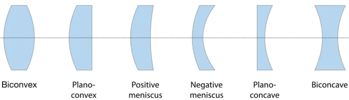
To understand the special characteristics of a Fresnel lens, conventional lenses have to be examined first. The first possible classification of simple lenses is made by the type of curvature of the two optical surfaces, the light will pass (cf. figure 4.1). While theoretically, each of these lenses can be used in both orientations (light coming from the left side and light coming from the right side), the optimal usage of a lens depends on application situation. A lens produces less spherical aberration (see section 4.1.3.1), if the angle of incidence Φ (cf. figure 4.9 in section 4.1.3) of the light (in particular marginal rays) on both optical surfaces is small. In case of focussing a collimated beam of light, a plano

Each category is further subdivided into spherical and aspherical lenses. The former is characterised by the special parameterisation of its surfaces, both being part of a sphere, while the surfaces of aspheric lenses in most cases follow optimised parameterisations to correct monochromatic aberrations. Another way to correct aberration is the usage of compound lenses, i.e. an array of simple lenses with a common axis. As both methods lead to the same result, one aspherical lens can achieve the optical performance of a system consisting of 3 ~ 4 spherical lenses [26]. Nevertheless, the use of compound lenses is often preferred for financial reasons if space and weight is not a limiting factor. The lens surface is rotationally symmetric with respect to the optical axis, thus the aspheric profile of a lens can be parameterised using the sagitta function with cylindrical coordinates [26]:

Here, z describes the thickness of the

lens along the optical axis, ρ describes the axial radius perpendicular to the optical axis, R denotes the bending radius of curvature and k is the conic constant.

The coefficients C_i are aspherical deformation constants that represent a perturbation to the conic surface profile. Possible surface profiles depending on the conic constant without aspherical perturbation result from the intersection of a conical surface and a plane, illustrated in figure 4.3.

Figure 4.1: Different types of lenses categorised by the form of both optical surfaces.

Figure 4.2: Construction of a lens surface with cylindrical coordinates. Three different profiles with the same radius of curvature R were used: green spherical, brown parabola and blue parabola including

aspherical deformation constants Ci which were optimised for the fluorescence telescope FAMOUS.

R = 26.37cm

ρ

k

= 0

k

= -1

k

= -1

z

Optical axis 10 20 30 -10 -20 -30

/cm

/

cm Biconvex

Plano-convex meniscusPositive meniscusNegative concavePlano- Biconcave

For the fluorescence telescope FAMOUS, an optimal set of parameters was obtained by using the commercial optics design software Zemax [18]. The optimisation process in this software is based on the minimisation of a definable “merit-function”, which consists of operands representing individual qualities of the optical system, which needs to be optimised. Each operand holds a “target” and a “weight”, which give the ability to set a desired value, and the corresponding relative importance for that quality in comparison to the other attributes of the system. This feature is necessary for the optimisation of optical systems, as the only perfect optical device is a plane mirror. All other optical components and systems have to be optimised for the individual operating range. The optimised lens profile for FAMOUS, which describes the conventional, i.e. “bulky” counterpart to the desired Fresnel lens, is shown in figure 4.2 in comparison to a parabola and a spherical profile with the same radius of curvature. The deformation constants are listed in table 2. Since the production of a Fresnel lens with an individual aspherical surface profile is rather expensive, a similar prefabricated Fresnel lens was used for the studies in this thesis.

Figure 4.3: Conic sections are formed by the intersection of a cone surface and various planes. In blue: parabola, circle and ellipse, in yellow: hyperbola.

Constant Value

C₁ 1.18 · 10-4 _m-1 C₂ 1.34 · 10-9 _m-3 C₃ 9.52 · 10-15 _m-5 C₄ -2.04 · 10-19 _m-7 Table 2: Deformation constants of the lens surface profile for the fluorescence telescope FAMOUS. Taken from [18].

4.1.1 Point spread function

One of the most important quality criteria for imaging performance is the image resolution. In case of a lens, the image resolution quantifies how close two point like objects can be to each other and still be differentiated on the image plane. This is closely related to the point spread function (PSF), which is the intensity distribution on the image plane of the focal point of the lens.

The point spread function is a measure for the ability of the lens to focus light on a single point which also depends on the application situation, leading to different aberration effects, discussed in section 4.1.3. The influence of the point spread function on the process of image formation is explained in the following section.

In a more general approach, the PSF is the two-dimensional response function of a focussed optical system. In this approach, the lens in combination with the image plane is a dynamic system, that gives a characteristic response to an input signal, which is the light - reflected or emitted - by an object, for example the fluorescence light of an extensive air shower. To study the characteristic response, a preferably simple input signal (an impulse) is presented to the system [27]. In general, the choice of an appropriate impulse is not trivial and depends on the nature of the system.

In the case of non-coherent linear imaging optics, with the aim to reproduce an object plane on an image plane (see figure 4.4), the formation process of an image follows the superposition principle, which is due to the non-interacting property of photons and can be described by linear system theory [27]:

For this reason, the object plane O(x,y) can be subdivided into infinitesimal portions at locations (x₀ ,y₀), i.e. many individual objects (figure 4.4) performing a convolution with a two-dimensional Dirac delta function:

x

₀

y

₀

x

x‘

y

y‘

Optical axis d

x

_i

y

_i

f

f

G

B

g

b

Figure 4.4: Image formation of a refractive optical system. The object plane can be subdivided into

indi-vidual points with coordinates (x₀ , y₀), which are translated to the image plane with distance from lens to

object plane and lens to image plane of g and b, respectively, and the focal length f, which is identical on both sides of the lens. The distance of a point on the object plane from the optical axis is denoted as G while the distance from the optical axis to the transferred point is denoted as B. The coordinate system of the image plane is reversed from the object plane coordinate system.

(16)

The coordinates of each point of the object plane can then be translated into coordinates on the image plane (figure 4.4) with the knowledge of the focal length f of the used lens and a given object distance g, contained in the magnification M for a focussed system:

Each point of the object plane O(x₀,y₀) is individually mapped on the image plane, including the response of the lens, the PSF. As a result, a characteristic blur is added to each image point, overlapping with nearby image points (figure 4.5). The total resulting image I(x_i,y_i) is formed by the superposition of the images from all object points [27]:

The magnification M needs to be included to translate between the coordinates of the object plane and the image plane. Precisely, the total image can be expressed as the weighting function of the object plane, convoluted with the impulse response function, which is the image of the Dirac function. The Dirac function is the mathematical analogon to a point light source.

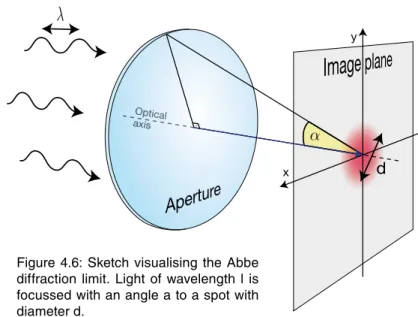
4.1.2 Diffraction limit

The size of a focal point is mainly influenced by geo-metrical imperfections of the surface of a lens. While un-corrected lenses suffer from several aberration effects, the imaging performance of modern aspheric corrected lenses is limited only due to the diffraction of light. This is one of few directly visible consequences of quantum mechanics and was the

inspi-ration for Heisenberg’s quantum uncertainty principle [28]. An optical system, with an angular resolution that is limited by diffraction effects is called diffraction limited. Figure 4.5: Graphical representation of equation 19: The image is formed by convolution of the original picture of the object and the PSF of the optical system. The PSF is the image of a point light source.

(18) (19) d x y Optical axis α

Figure 4.6: Sketch visualising the Abbe diffraction limit. Light of wavelength l is focussed with an angle a to a spot with diameter d.

0.0 0.0 0.5 1.0 -0.5 -1.0 0.5 1.0 -0.5 -1.0 0.2 0.4 0.6 0.8 Y in µm X in µm Rel . intensit y σ = 0.13 Nor malised r

el. intensity, contained po

wer 0.0 0.5 1.0 1.5 2.0 2.5 3.0 0.9 1.0 0.8 0.6 0.4 0.2 0.0 6 12 18 24 I C

R90

x = π D sin(β) / λ Radius in µm

R90

Figure 4.7: Airy pattern on the image plane for a circular aperture with D = 2a = 549.7 mm diameter, focal

length f = 502.1 mm and light with λ = 350 nm wavelength. The grey plot represents the relative intensity

distribution as a function of radius using the dimensionless variable x = πD sin(β) / λ and for comparison

the radius is also plotted in µm. The dashed blue line denotes the integrated encircled energy as a function of the radius. The black dashed line resp. green dashed circle in the equivalent 3d surface plot The minimum spot size d of light with wavelength λ, focussed with an angle α, in a medium with refractive index n is given by the Abbe diffraction limit (cf. figure 4.6):

The point spread function for such a system with circular aperture and infinitely distant point light source is known as Airy pattern [29],

which is shown in figure 4.7. It is a special case of the more general Fraunhofer diffraction pattern. Here J₁(x) is the Bessel function of the first kind of order one and x is a dimensionless variable which contains not only the radius a of the aperture, i.e. the

lens, and the wavenumber k = 2π/λ of the light, but also includes the incident angle β of

β (21)

the light rays on the image plane, illustrated in figure 4.8. For small angles β, x can be approximated with the distance r to the optical axis in the image plane:

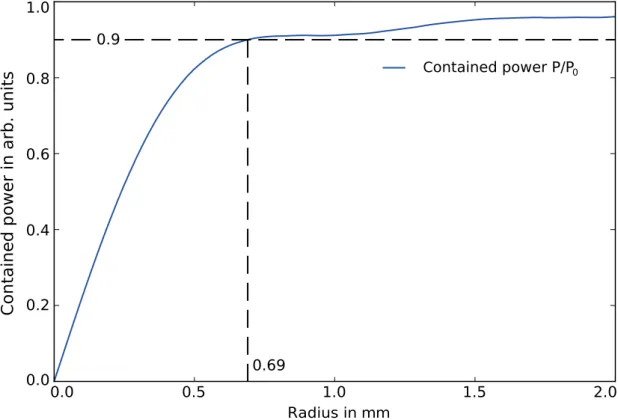
In the center of the Airy pattern, a blurry spot is formed, also named Airy disk or circle of least confusion with a maximum intensity I₀, surrounded by altering dark and bright rings caused by constructive and destructive interference. In figure 4.7, the Airy pattern is plotted as a function of x but also as a function of r for the aperture parameters describing the “bulky” counterpart of the Fresnel lens of FAMOUS.

A significant value for the size of the Airy pattern is the radius of a centered circle on the image plane, which encircles a certain portion of the total integrated intensity. In figure 4.7, the radius for 90% encircled energy is shown. It is referred to as R90 (see section 4.2.5) and is also used to describe the size of the point spread functions measured for the Fresnel lens in chapter 8. Note that the peripheral rings contain a significant portion of the total intensity, while radial intensity tends against zero. This is due to the encircled area, which increases with the square of the radius. Not only theoretically but also practically, the point spread function will never drop to absolute zero in its intensity rings even for infinite distance to the center of the spot.

An alternative method to determine the size of the point spread function is a Gaussian fit to the pattern. The size is then given by the width of the Gaussian function

σ= 0.42λN = 0.13 µm in case of the the Airy pattern. The width σ is a factor of 5 smaller than the aberration radius R90 = 0.67 µm.

β

r

x

y

f

Optical axis

θ

a

Figure 4.8: Airy pattern on the image plane for an aperture with radius a and focal length f. Radial distances to the optical axis can be described by using

4.1.3 Aberrational effects

Apart from the theoretical limit on focussing light, which is given by diffraction, a series of other optical effects can cause a reduction of the imaging performance which are known as “intrinsic aberrations”. Additionally, a perfect alignment of all optical components is not possible in reality, resulting in further “externally induced aberration”. All effects, which deteriorate the image have to be incorporated in the detector response simulation and can be observed as a special pattern or dependency of the PSF, which can be explained due to deviations from spherical geometry of the shape of the wave front which is formed by the lens (figure 4.9).

The standard lensmaker’s equation, connecting the surface curvature of the lens with the focal distance is based on the series expansion of the sines in Snell’s law [27]:

with the angle of incidence Φ and refraction Φ’ of light passing through a boundary of different isotropic media with refractive indices n and n’. The replacement of the sines is also called paraxial or Gaussian approximation, as it is only valid for rays, which are close to the optical axis, called paraxial rays (figure 4.9). This approximation leads to a quick and practical way to determine paraxial focus, but does not provide any information on aberrations, while the Seidel approximation also includes the second term in the sine series expansion:

which can be used to describe primary or third order aberrations like spherical aberration, coma, astigmatism and field curvature. In the following, the different aberrational effects for conventional lenses will be presented, to understand their impact on the PSF.

Figure 4.9: Spherical wavefronts formed by a perfect lens (top) and (spherical) aberrated wavefronts of an imperfect lens (bottom). The wavefront error describes the deviation of the refracted wavefront from a spherical surface. The aberrated rays intersect at different longitudinal distances along the optical axis as well as transversal distances in the focal plane. The resulting intensity distribution on the image plane for the aberrated case is described by the point spread function and its radial size characterised by the

aberration radius R90. The angle between lens surface normal and parallel incoming light is marked as Φ.

Upper half: perfect case Bottom half: aberrated case Wavefront error Angular error Paraxial rays Marginal r ays Image plane transversal Paraxial focus longitudinal Incoming wavefronts Optical axis Lens Surface normal

Φ

R90 Intensity distribution

90%

(23) (24)

4.1.3.1 Spherical aberration

Spherical aberration describes the effect, that incident rays closer to the edge of a lens (marginal rays) are bent too strong in comparison to rays passing the center (figure 4.9), resulting in different crossover points along the optical axis. This effect appears for spherical lens surfaces, as those do not form spherical wave fronts. The longitudinal aberration is given by the distance between the focal point for paraxial rays and for peripheral rays, also called marginal focus. The best focus locates right between paraxial and marginal focus.

4.1.3.2 Coma aberration

This aberration affects off-axis image points. For these, incoming wavefronts are tilted with regard to the optical axis. The resulting wavefront aberration after refraction is shown in figure 4.10 on the bottom left, which forms a comet like blur on the image plane. At point F_b, the maximum intensity is located, while the Gaussian image point is located at point B. The coma blur is created by progressively expanding circles along the axis of aberration a. Inner circles coincide with the paraxial focus, while the biggest circles are formed by the edge of the lens.

1 2 3 4 1 2 3 4 _1’ 3’ 1’ 2’ 3’ 4’ 2’ 4’ 0 1 2 3 3’ 4 1’ 2’ 4’ 60° 0 r 1 1’ 1 1’ 1 1’ Tilt corrected reference sphere Wavefront error Lens Points on lens Points on image plane _B Fb a a 0 0

Figure 4.10: Sketch of the geometrical construction of comatic aberration. Different points of two circles on the lens are numbered and their contribution to the comatic blur on the image plane is illustrated. A cross section of the wavefront error in comparison to the tilt corrected reference sphere is also shown on the bottom left. Inspired by [27].

4.1.3.3 Astigmatism

As coma aberration, astigmatism is also caused by inclined incident wavefronts. To understand this effect two imaginary planes have to be introduced: the tangential plane is defined by the central ray and the optical axis, whereas the sagittal plane is orthogonal to it and includes the central ray, as shown in figure 4.11. Due to the incident angle, the projection of the incoming wavefront on the lens surface forms an ellipse. Since the focal length depends on aperture diameter, which for the ellipse is smallest at the intersection with the tangential

plane, and largest for the intersection with the sagittal

plane, the two orthogonal wavefront sections focus

at longitudinal separation. The circle of least confusion

is located between the two focal points T and S

(figure 4.11). T S Lens Circle of least confusion

Figure 4.11: Sketch of the geometrical construction of astigmatism. The projection of incoming wavefronts on the lens forms an ellipse which results in different aperture diameters as well as different focal lengths in tangential (green) and sagittal (magenta) plane with focal points T and S respectively.

4.1.3.4 Petzval field curvature

For most of the technical and practical applications, every point imaged by a lens should ideally be contained in the focal plane, containing a flat sensor to process the total image. In fact, the image of a lens is formed over a parabolic curved surface, described by a term called Petzval contribution PC, which is the distance from the flat to the curved image plane (figure 4.12):

with angle of incidence θ, focal length f and index of refraction

n of the lens. Nature solved that problem by developing the eyeball, simply fitting the retina to the curvature needed. As most small camera sensors can not be bent, this aberration

θ

PC

Lens

Petzval surface Paraxial image plane

f

x

Figure 4.12: The image of a sim-ple lens is formed over a curved (25)

4.2 Fresnel lens

4.2.1 Basic concept

A conventional lens of large diameter and high refraction power becomes relatively bulky and can contain several kilograms of material. However, crucial for the light refraction is only the relative angle of the two active surfaces of a lens. The idea of a Fresnel lens is to divide the lens into a set of concentric annular sections called “grooves” and save as much material as possible while the curvature of the active surfaces remains unaffected, see figure 4.13.

Groove

ρ

z

(

ρ

)

Slope angle

Lens

Fresnel lens

aj aj+1 δ

Figure 4.13: Basic construction principle of a Fresnel lens. The bulky lens is divided into a set of concentric annular “prisms” which are named “grooves”. The curvature of the active optical surface still follows the

sagitta function (section 4.1) but is approximated by linear segments described by a slope angle δ.

The major disadvantage of this concept results from the stepwise discontinuities in surface between the grooves. Light rays which are bent towards an inactive face that connects two grooves are disturbed due to total internal reflection or additional false refraction as shown in figure 4.14. On top of that, the aberrations of conventional lenses, discussed in the previous section, are also present for Fresnel lenses although the process of manufacturing makes it easier to correct for spherical aberration.

4.2.2 Manufacturing

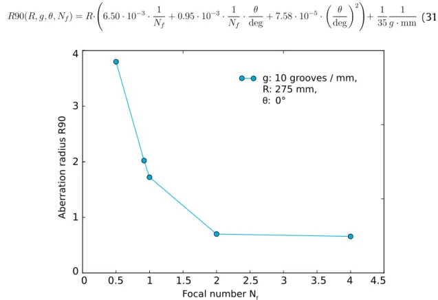
The Fresnel lens used for the fluorescence telescope FAMOUS is made by compression molding of PMMA3_{. The mold cavity facet geometry is usually cut by a precision diamond} tool with a straight cutting edge. Therefore, the active optical surface of the grooves is a flat approximation of the curved lens surface and can be described by a successivly increasing slope angle δ towards the outer region of the lens (figure 4.13). The draft angle ψ also increases with distance to the center of the lens to enhance the transmittance of light, which is refracted near the top edge of a groove (figure 4.14, red dashed light beam). To achieve best transmittance, the angle a₁ (figure 4.14) has to tend to zero. Each of the grooves is individually engraved into the mold, which makes it possible to generate any spherical or aspherical surface profile. It is even possible to generate a groove based on its individual profile, so that every groove on the Fresnel lens is part of a different surface profile. This leads to a maximum degree of freedom to design a lens for special applications [22]. The filling process of the mold cavity is a complicated process because of high temperature and pressure gradients. The Fresnel lens is about 2 mm thick but contains facet structures in the mircometer range. These structures will only be filled with the polymer when it is sufficiently pressurised. The temperature of the filled polymer melt is significantly higher than the temperature of the mold cavity, resulting in a cool down of the polymer after the filling process accompanied by a viscosity increase, which in turn requires additional time dependent pressure control [30].

Figure 4.14: Cross section of a groove with relatively high slope angle δ. The fraction of correctly refracted

light rays in comparison to the total incoming light gives a first hint on the transmittance of the Fresnel lens.

Active face

Groove

Incoming rays

Peak rounding

Slope angle Draft angle

Inactive face

δ

ψ

After the filling process is completed, the polymer has to be cooled and solidified. This step as well as the ejection of the cooled lens from the mold have to be performed in a correct manner to avoid additional stress. The quality of all process parts has direct im-pact on the performance of the lens. If the pressure after filling the melt into the mold is not high enough or is executed too late, the groove edges are not filled correctly and a rounded groove peak (figure 4.14) is formed, which in consequence reduces imaging quality and transmittance performance [30].

4.2.3 Diffrac