Optimal Unemployment Insurance
with Monitoring and Sanctions
¤
Jan Booney Peter Fredrikssonz Bertil Holmlundx Jan van Ours{
This version: 2 November 2001
Abstract
This paper analyzes the design of optimal unemployment insur-ance in a search equilibrium framework where search e¤ort among the unemployed is not perfectly observable. We examine to what extent the optimal policy involves monitoring of search e¤ort and bene…t sanctions if observed search is deemed insu¢cient. We …nd that intro-ducing monitoring and sanctions represents a welfare improvement for reasonable estimates of monitoring costs; this conclusion holds both relative to a system featuring inde…nite payments of bene…ts and a system with a time limit on unemployment bene…t receipt. The opti-mal sanction rates implied by our calibrated model are much higher than the sanction rates typically observed in European labor markets.
JEL-classi…cation: J64, J65, J68
Keywords: Unemployment insurance, search, sanctions
¤We thank seminar participants at IZA, Bonn, for comments on an earlier draft of the
paper. Financial support from the Swedish Council for Working Life and Social Research is gratefully acknowledged.
yDepartment of Economics and CentER for Economic Research, Tilburg University,
OSA and CEPR. Postal address: Box 90153, 5000 LE Tilburg, The Netherlands. E-mail: j.boone@kub.nl
zDepartment of Economics, Uppsala University, IFAU and CESifo. Postal address:
Box 513, SE-751 20 Uppsala, Sweden. E-mail: peter.fredriksson@nek.uu.se
xDepartment of Economics, Uppsala University and CESifo. Postal address: Box 513,
SE-751 20 Uppsala, Sweden. E-mail: bertil.holmlund@nek.uu.se
{CentER for Economic Research, Tilburg University, OSA, IZA and CEPR. Postal
1
Introduction
It is generally accepted that public provision of unemployment insurance (UI) is socially desirable in a world with risk averse individuals. However, it is also well established that the provision of UI does not come without adverse incentive e¤ects. For example, more generous UI bene…ts is likely to reduce search e¤ort and raise wage pressure, thus causing some increase in unemployment. The problem facing policy makers is thus to strike an opti-mal balance between the insurance bene…ts on the one hand, and the adverse incentive e¤ects on the other hand. This problem has been the subject of several recent papers. Our paper contributes to this literature by recogniz-ing that the government may condition bene…t payments on (imperfectly) observed search e¤ort. This leads us to an analysis of optimal UI design in a search equilibrium framework where the government has several policy instruments at its disposal, including the bene…t level, the rate at which search e¤ort is monitored, and the magnitude of the sanction in case search e¤ort is regarded as insu¢cient. We …nd that a system with monitoring and sanctions represents a welfare improvement relative to other alternatives for reasonable estimates of the monitoring costs.
Our resuls on the desirability of monitoring can be contrasted with a wellknown result that dates back to Becker’s (1968) celebrated paper on optimal crime deterrence. In Becker’s analysis (as in ours), monitoring is costly because resources have to be spent on detecting crime (violations of search requirements). Punishment, in the form of a …ne (sanction), goes without cost since it involves a transfer of money from one individual to others. To deter crime the expected …ne, i.e., the probability of being caught times the …ne, should be big enough. By raising the …ne, monitoring costs can be reduced without a¤ecting incentives for crime. However, Becker’s analysis presupposes risk neutral agents. When agents are risk averse, as they are in our model, Becker’s result need not hold. The reason is that a very high …ne would lead to a substantial welfare loss for agents who violate the law.1
The seminal papers on optimal UI appeared in the late 1970s (Baily, 1978; Flemming, 1978; Shavell and Weiss, 1979). The paper by Shavell
1See Garoupa (1997) and Polinsky and Shavell (2000) for recent surveys of the economic
theory of law enforcement. The recent literature in this …eld has shown, inter alia, that
allowing for risk averse agents would weaken the classic Becker argument and suggest a case for costly monitoring.
and Weiss (1979) analyzed the problem of optimal sequencing of bene…t payments over the spell of unemployment. The key result was that the bene…t level should decline monotonically over the unemployment spell, because such a pro…le involves stronger incentives to search. The recent paper by Hopenhayn and Nicolini (1997) has extended the analysis in Shavell and Weiss by considering a wage tax after reemployment in conjunction with the sequence of bene…t payments. The basic results are twofold: …rst, bene…ts should decrease over elapsed duration, as in Shavell and Weiss; second, the wage tax should increase with the length of the previous unemployment spell. These two papers o¤er a partial analysis in the sense that workers’ wages are given. A few recent contributions have also allowed for endogenous wage determination. Cahuc and Lehmann (2000) propose a model where …rms and unions bargain over wages and notice the possibility that a declining time pro…le may raise wage pressure by strengthening the power of “insiders” in the wage negotiations. This rise in wage pressure tends to o¤set the positive search incentives arising from a declining time pro…le. The paper by Fredriksson and Holmlund (2001) analyzes optimal bene…t sequencing in a model of search unemployment along the lines of Pissarides (1990). The model features endogenous search e¤ort, endogenous wage determination and free entry of new jobs. The analysis shows analytically that a declining time pro…le of bene…t payments is optimal, provided discounting is ignored. With discounting, numerical calibrations suggest that the wage pressure e¤ect is not strong enough to o¤set the favorable e¤ect on search incentives.
The contributions reviewed above, and most of the other literature on optimal UI, do not consider that the government can make the receipt of bene…ts dependent on the unemployed worker’s search e¤ort. As documented by Grubb (2001), existing UI systems condition bene…t payments on perfor-mance criteria such as “availability for work” and “active job search”. These criteria are enforced by some degree of monitoring of the bene…t claimants. The requirements for job search show substantial variations across countries. Failure to meet search requirements may result in a bene…t sanction, i.e., a temporary or permanent cut in bene…ts. A typical duration of sanctions for a …rst refusal of a suitable job o¤er is two to three months. Observed sanction rates – the total number of sanctions over a year relative to the stock of bene…ciaries – also vary substantially across countries. For example, sanctions due to insu¢cient search hovered around 30 percent in the United States in the late 1990s, whereas other countries (Germany, Denmark, Nor-way) appear to have undertaken no sanctions related to search inactivity.
See Grubb (2001) for further details.
Recent empirical work has shed light on the e¤ects of changes in search requirements and monitoring of job search. The arguably most convincing ev-idence is based on randomized experiments undertaken in the United States. The “treatments” in these experiments involved the number of employer con-tacts, the required documentation and the frequency of veri…cation.2 These
studies indicate that either more intensive monitoring or more demanding search requirements tend to reduce the length of bene…t claims. Recent non-experimental evidence from the Netherlands also suggest that the imposition of sanctions substantially raises the transition rate to employment (Abbring et al, 1997; van den Berg et al, 1998). All in all, our reading of the bulk of the evidence is that more intensive monitoring and more stringent search requirements do matter for search activity and transitions out of unemploy-ment.3
The economics literature on monitoring and sanctions in the context of UI is very small. The study most closely related to what we do in the present paper is Boone and van Ours (2000). The model is a version of the Pissarides (1990) search and matching model and has similarities with the model in Fredriksson and Holmlund (2001). Workers are risk averse, search e¤ort among the unemployed is endogenous and wages are determined in bargaining between the …rm and the individual worker. A key assumption is that the unemployed and insured worker can a¤ect the probability of contin-ued UI receipt by the choice of search e¤ort; the higher the search e¤ort, the lower the risk of being exposed to a bene…t sanction. This is the monitoring system in the model. The bene…t associated with additional search thus in-volves two components, one capturing the gain associated with a transition to employment and the other capturing the gain of not being penalized by a bene…t sanction.
The purpose of this paper is to extend the earlier contributions by Boone and van Ours (2000) and Fredriksson and Holmlund (2001) so as to incor-porate an analysis of an optimal bene…t system with costly monitoring and sanctions. The basic model features two bene…t levels which can be thought
2See OECD (2001), Johnson and Klepinger (1994), Benus et al (1997) and Black et al
(1999).
3There is at least one study, van den Berg and van der Klaauw (2000), that fails to
con…rm that more intensive monitoring a¤ects transitions out of unemployment. The authors conjecture that the result may re‡ect that more stringent monitoring of formal search induces a substitution away from informal search channels.
of as unemployment insurance (UI) and unemployment assistance (UA), re-spectively. Workers who receive UI are monitored at a certain rate and, with some probability, exposed to a bene…t sanction. The probability of being sanctioned depends on the worker’s search e¤ort and the precision at which search e¤ort can be observed by the UI provider. Sanctioned workers receive UA, they are not monitored, and they need to become reemployed before they are entitled to UI. We are concerned with the characteristics of the op-timal bene…t system when there are four available policy instruments: the level of bene…ts in UI and UA (the di¤erence between the two representing the sanction), the rate at which the unemployed worker entitled to UI is monitored, and the precision of the monitoring technology that determines how the agent’s search e¤ort a¤ect the probability of a sanction.
The next section of the paper presents the basic model. Section 3 de-rives some analytical results concerning the properties of the optimal bene…t system. In section 4, we turn to a numerical analysis of the optimal bene…t system. Section 5 concludes.
2
The Model
2.1
The Labor Market
We consider an economy with a …xed labor force, which is normalized to unity. Workers are either employed or unemployed and have in…nite horizons. Time is continuous. An employed worker is separated from his job at an exogenous Poisson rate Á. Upon entering unemployment, the worker is immediately eligible for UI bene…ts.
Recipients of UI bene…ts are monitored with respect to their search be-havior. If they fail to meet certain search requirements, they are exposed to a bene…t withdrawal (a sanction). We assume that the sanction lasts for the remainder of the unemployment spell. At every instant, there are thus two groups of unemployed workers: eligible workers who receive bene…ts and
sanctioned workers who have been exposed to a bene…t withdrawal.
Let®j, j =e; sdenote the exit rate from unemployment to employment
for an eligible and a sanctioned worker, respectively. The exit rates di¤er between the two groups to the extent that their search e¤ort di¤er. Let sj,
j =e; s, denote search e¤ort. The e¤ective number of searchers in the econ-omy is then given asS =seue+ssus, whereuj is the number of unemployed
in category j.
The matching function, which is of the usual constant returns to scale variety, is given by H = H(S; v), where v is the number of vacancies. Let
µ ´v=Sdenote labor market tightness. The probability per unit time that in-dividualiescapes unemployment statej is then obtained as®ji ´s
j
iH(S; v) =
sji®(µ). Also, ®(µ) = H(S; v)=S = H(1; µ) and hence ®0(µ) > 0; the tighter the labor market, the easier to …nd a job. Firms …ll vacancies at the rate
q(µ) = H(S; v)=v = H(1=µ;1), and thus q0(µ) < 0; the tighter the labor market, the more di¢cult to …ll a vacancy. By constant returns to scale, we also have ®(µ) =µq(µ).
While unemployed and receiving UI bene…ts, an unemployed agent is monitored at rate ¹. We think of monitoring as random inspections of the worker’s search activity. Given monitoring, there is some probability that the observed search e¤ort does not meet the search requirement, in which case the worker is sanctioned. Let ¼(se) denote the probability of being
sanctioned upon inspection of search e¤ort, implying that UI recipients loose entitlement at the rate ¹¼(se).
Having de…ned the relevant transition rates, we can state the ‡ow equi-librium relationships of the labor market:
Án=®eue+®sus (1)
®sus=¹¼ue (2)
where n = 1¡ue
¡us denotes total employment in the economy. The …rst
equation pertains to employment whereas the second equation pertains to the state of unemployment with a sanction. Now we can use (1) and (2) to solve for employment:
n= ¸(®
e+¹¼)
Á+¸(®e+¹¼) (3)
where¸´ue=(ue+us) = ®s=(®s+¹¼))is the ratio of eligible unemployment to total unemployment.
2.2
Monitoring and Sanctions
Let us make the monitoring and sanctions technology explicit. We choose a reduced form speci…cation which allows us to have as special cases inde…nite payments of UI bene…ts (¹= 0), …nite duration of UI bene…t receipt (¹ >0
and ¼(se) = 1), and a sanction and monitoring technology. In particular,
we assume that the probability of being sanctioned upon inspection depends linearly on search: ¼(se) = 1
¡¾se. Proposition 2 below gives conditions
under which ¾ >0 is optimal. Further, we require that ¼(se)
¸ 0.
The parameter ¾ measures to which extent the sanction probability de-pends on an agent’s own search e¤ort. One way to interpret ¾ is that it indexes the precision of the inspection technology. For instance, ¾ = 0 cor-responds to the situation where it is determined by lottery if the agent has searched to rule or not; therefore everyone who is monitored is sanctioned irrespective of search intensity. Alternatively, ¾ = 0 can be seen as a UI system with a time limit, as in Fredriksson and Holmlund (2001). If, on the other hand, ¾ is strictly positive the agent’s search e¤ort matters for the sanction probability. The higher is ¾, the higher the precision with which an agent’s search e¤ort is observed and rewarded.4
Whereas¾ = 0gives little direct incentive to search, it is an inexpensive system to operate. This is due to the fact that there are no inspections of agents’ search e¤ort. On the other hand, ¾ > 0 gives a direct incentive to search but also implies that more monitoring o¢cials are needed in order to inspect agents’ search intensities. So the monitoring cost per monitored agent is increasing in ¾.
More precisely, we assume that the cost of running the monitoring and sanctioning system, C, is given by:
C =c(¾)¹uew (4)
The costs of running the UI-system are increasing in the number of moni-tored individuals (¹ue). The rate of increase is determined byc(¾)
¸0. This cost depends on the precision of the inspection technology withc0(¾)¸0and
c(0) = 0. We think of the inspection of search as a labor intensive activity
and, therefore, the monitoring cost is proportional to the aggregate wage w.
2.3
Worker Behavior
The employed worker’s (indirect) instantaneous utility is determined by his wage,w. The unemployed worker receives unemployment bene…ts,B, as long as he is eligible. When sanctioned, he receives Z. We show in proposition 1
4From a more general point of view, it is possible to derive this technology from ”…rst
below that B > Z. We assume that workers do not have access to a capital market, so consumption equals income at each instant.
We take the utility functions to be strictly concave in income and leisure. The unemployed worker’s instantaneous utility is decreasing in search e¤ort, since search reduces time available for leisure. The utility function for the eligible unemployed worker is À(B; se) and for the sanctioned worker it is
À(Z; ss). The employed worker’s utility is given by À(w; h), wherehdenotes
hours of work; we take h as exogenously …xed.
Let r denote the subjective rate of time preference and let Uj andE be
the expected present values of being unemployed, j = e; s, and employed, respectively. The value functions can then be written as:
rUe = max se fÀ(B; s e) +se®(µ) (E ¡Ue)¡¹¼(se) (Ue¡Us)g (5) rUs = max ss fÀ(Z; s s) +ss®(µ)(E ¡Us)g (6) rE = À(w; h)¡Á(E¡Ue) (7)
The unemployed worker chooses search e¤ort to maximizerUj, j =e; s.
The …rst-order conditions are given by:
Às(B; se) +®(µ)(E¡Ue)¡¹¼s(se) (Ue¡Us) = 0 (8)
Às(Z; ss) +®(µ)(E¡Us) = 0 (9)
where partial derivatives with respect to search e¤ort are indicated by sub-script s. In these expressions we have imposed symmetry, i.e., we have made use of the fact that workers are identical and choose the same search ef-fort. The …rst-order conditions convey the usual message:5 at the optimum,
the marginal cost of search should equal the marginal bene…ts. The mar-ginal cost is captured by foregone leisure, i.e., Às(B; se) and Às(Z; ss). The
marginal bene…t involves the gain in utility associated with a transition to employment, i.e., ®(µ)(E ¡Uj), j = e; s. For the eligible worker, there is
an additional bene…t of more intensive search, as revealed by the third term on the right-hand side of (8). More intensive search reduces the probability of being sanctioned, thus prolonging the expected duration of bene…t pay-ments. This does not imply, however, that eligible workers necessarily search harder than sanctioned workers. The e¤ect pulling in the opposite direction
5The second-order conditions for a maximum are ful…lled by the concavity ofÀ(¢)and
is B > Z: sanctioned workers gain more from …nding a job than eligible workers sinceE¡Us > E¡Ueholds in equilibrium. Which e¤ect dominates depends on the parameters of the UI system.
We assume that the instantaneous utility functions take the form:
À(m; l) = lnm+ ¡(l); m=fw; B; Zg; l=f1¡¹h;1¡se;1¡ssg
where mdenotes (real) income, which depends on the worker’s labor market position. The employed worker recieves a wage w; the eligible unemployed worker receives unemployment insurance,B; and an unemployed worker who has been exposed to a sanction receives unemployment assistance, Z. Fur-thermore, ¡(l)represents the value of leisure with ¡0(l)>0 and ¡00(l)<0.
2.4
Firms and Wage Bargaining
Assume that government expenditure on bene…ts and monitoring is …nanced by a proportional payroll tax paid by …rms. Labor productivity is constant and denotedy. The cost of holding a vacancy isky, withk > 0. LetV denote the present value of a vacant job andJ the present value of an occupied job. The value functions are of the usual form:
rV =¡ky+q(µ)(J¡V) (10)
rJ =y¡w(1 +t)¡Á(J¡V) (11)
wheretis the proportional payroll tax rate. With free entry of new vacancies,
V = 0, we obtain the wage cost as proportional to the marginal product of labor, i.e.,
w(1 +t) = [1¡(r+Á)k=q(µ)]y (12)
De…ning wc ´ w(1 +t) and writing the right-hand side of this equation as
d(µ)y; we refer towc=d(µ)y as the zero pro…t condition, with d0(µ)<0.
The outcome of the Nash bargain
max wi [E(wi)¡Ue] ¯ [J(wi)¡V] 1¡¯ ; ¯2(0;1)
is a relationship of the form:
E¡Ue wÀw = ¯ 1¡¯ J wc (13)
where V = 0 and symmetry have been imposed. The Nash bargain implies a wage-setting relationship, i.e., a relationship between bargained wages and labor market tightness. We assume that the government …xes the replace-ment rates in this economy. Hence Z = zw and B = bw where z and b
are policy parameters. The replacement rates are de…ned with respect to the economy-wide average wage which the individual employee perceives to be independent of his wage demands; therefore @Ue=@w = 0. Finally, the
relative size of the bene…t sanction is denoted byp, i.e. psatis…esz = (1¡p)b:
2.5
Equilibrium
Our assumptions imply that the model has a convenient recursive structure; the model in Fredriksson and Holmlund (2001) has a similar structure. The zero-pro…t condition and the wage-setting relationship determine µ andwc.
To see this, note that with free entry of vacancies we have J =ky=q(µ) and
wc = d(µ)y, which imply that the right-hand side of (13) is increasing in µ
but independent of sj. Moreover, the left-hand side of (13) is a function of
µ but independent of w given our chosen utility function and the fact that income during unemployment is proportional to the aggregate wage. It can also be shown thatE¡Ue is independent ofsj, an envelope property implied
by optimal search behavior. With µ determined, we get sj from (8) and (9), since the di¤erences in present values are independent of w. With µ andsj
determined, we obtain uj andnfrom (1)-(3).
Notice that µ, wc, sj, uj and n are independent of the tax rate, t. The
latter can be determined residually from the government’s budget restric-tion, noting that the government uses the wage tax to …nance bene…ts and monitoring costs:
twn=uebw+uszw+c(¾)¹uew (14)
With the tax rate determined, the worker’s take-home wage is obtained from
w=wc=(1 +t).
3
Optimal Unemployment Insurance
The optimal unemployment insurance system involves four instruments: b,
p, ¹, and ¾. We use a utilitarian welfare function, i.e., welfare (W) is de-…ned as: W = uerUe +usrUs+n(rE +rJ) +vrV where V = 0 by the
free entry condition. We ignore discounting; hence it is valid to compare alternative steady states without considering the adjustment process. With no discounting, the welfare objective simpli…es to an employment-weighted average of instantaneous utilities, i.e.
W =nÀ(w; h) +ueÀ(B; se) +usÀ(Z; ss) (15)
The optimal policy maximizes (15) subject to the market equilibrium conditions, sj = sj(b; p; ¹; ¾) and µ = µ(b; p; ¹; ¾), as well as the balanced
budget constraint, t = t(b; p; ¹; ¾). Let ½ = fb; p; ¹; ¾g denote the vector of policy parameters. Hence the vector of …rst-order conditions is given by
(dW=d½) = 0:
Before proceeding to the numerical results it is useful to state two an-alytical results. First of all, the key result in Fredriksson and Holmlund (2001) applies directly. The following proposition reiterates proposition 2 in Fredriksson and Holmlund (2001)
Proposition 1 The optimal policy involves p >0, provided that an interior solution to dW=db= 0 exists.
Proof. The proof is by contradiction. Suppose b > 0 and consider the trial solution p = 0: At p = 0; the …rst-order condition for ¾ has a solution at ¾ = 0 because c0(¾)¸ 0. Moreover, the condition for ¹is irrelevant. So, let us …x ¹ at some arbitrary, but interior, value: ¹0
2 (0;1): The uniform bene…t structure (p = 0) cannot be optimal if(dW=dp)> 0 at p= 0: Some manipulations of the …rst-order condition for pusing dW=db= 0 yields
µ dW dp ¶ p=0 = @W @ss @ss @p >0 (16)
where @W=@ss >0 denotes the partial derivative of welfare with respect to
ss holding µ constant, and @ss=@p >0 is, again, de…ned holding µ constant.
There are two key mechanisms that yield the sign of (16): there is a tax-ation externality associated with search and there is an “entitlement e¤ect”. The taxation externality derives from the fact that, given that some insurance is optimal (b >0), taxes are required to …nance unemployment expenditure. Individuals, however, do not take into account that taxes can be lowered if search intensity (and hence employment) increases. Therefore, @W=@ss >0:
Moreover, the so called entitlement e¤ect (c.f. Mortensen, 1977) will operate in this setting. Increasing the penalty will be conducive to search among those who are sanctioned since individuals will be eager to …nd a new job in order to qualify for (to be entitled to) UI bene…t receipt. As a corollary to proposition 1, the optimal policy will involve an interior ¹. In other words, the two tiered bene…t structure, b >0,p >0, and¹2(0;1), dominates the uniform bene…t structure in welfare terms.
Another interesting question is whether it will be optimal to have the sanctioning rate depend on search intensity, given an optimal choice of b,
p, and ¹: Since the inspection of search is the de…ning characteristic of the monitoring and sanctions system in this setting, we can equally well phrase the question as: Given an optimal choice of a UI system with time limits, is it optimal to introduce a system of monitoring and sanctions? The following proposition gives the condition when the answer turns out to be a¢rmative Proposition 2 Let ^½=fb; p; ¹; ¾ = 0g denote the solution to the restricted problem of optimal UI design. Then, the optimal policy will involve ¾ > 0 if
µ b ¹ ¸+ (1¡¸)(1¡p) ¸se+ (1¡¸)ss @se @¾ ¶ ½=^½ > c0(0)
Proof. The proof proceeds as follows. Given that the two-tiered bene…t structure is optimal, there are interior solutions to the …rst-order conditions
(dW=db) = 0,(dW=dp) = 0, and(dW=d¹) = 0:A UI system with monitoring
and sanctions must be optimal if (dW=d¾) > 0 at the point where ¾ = 0
and the remaining …rst-order conditions hold. Some manipulations of the …rst-order condition for ¾ using (dW=d¹) = 0 yields
dW d¾ = @W @se @se @¾ ¡ c0(0)¹ue (1 +t)n (17)
where @W=@se >0 denotes the partial derivative of welfare with respect to
se holding µ constant, and @se=@¾ > 0 is also de…ned holding µ constant. Introducing the explicit expression for @W=@se and rewriting slightly:
sign ½ dW d¾ ½=^½ ¾ =sign (µ b ¹ ¸+ (1¡¸)(1¡p) ¸se+ (1¡¸)ss @se @¾ ¶ ½=^½ ¡c0(0) )
Equation (17) illustrates the basic trade-o¤ in introducing a monitoring and sanctions system. A monitoring and sanctions system restores the search incentives among the eligible, @se=@¾ >0: Again, this is a good thing since
there is a taxation externality which is not taken into account in the private determination of search. However, inspecting search consumes real resources as indicated by the second term in (17). If this cost is su¢ciently high, the monitoring and sanctions system will not be introduced.6
Proposition 2 relates to the result in Boone and van Ours (2000). Their key result is that a monitoring and sanction system will be more e¢cient in restoring search incentives than overall bene…t reductions. This result is derived by means of numerical solutions to a model which is essentially identical to the present one, but with c0 = 0. Proposition 2 shows that their conclusion holds analytically. In addition it extends their result further: given c0 = 0; a system with monitoring and sanctions will dominate the two-tiered bene…t system analysed by Fredriksson and Holmlund (2001).
By inspection of (16) and (17), the extent that search responds to incen-tives is going to be crucial for the amount of bene…t di¤erentiation and the argument for introducing monitoring and sanctions.
4
Numerical Analysis
We have calibrated the model numerically so as to provide some information on plausible numbers. The basic time unit is taken to be a quarter and the matching function is Cobb-Douglas, H = aS1¡´v´, where we set ´ =
0:5.7 We …x hours of work exogenously to h = 0:75 and use the following
parameterization of the value of leisure:
¡(l) =Âl
·
¡1
· (18)
where · <1. The marginal product of labor is normalized to unity and we impose the Hosios (1990) e¢ciency condition ¯ =´.
We calibrate the model for a uniform bene…t system (p = 0) with a replacement rate of b = 0:3: The parameters a and  are chosen with an
6If introducing a sanction system involves a …xed set-up cost (besidesC), then clearly
the set-up cost should not be too big either.
7Broersma and Van Ours (1999) give an overview of recent empirical studies of the
eye towards vacancy duration and search intensity. We set a = 1:7 and = 0:6. Remaining parameters (k; ·; and Á) are calibrated such that expected unemployment duration is one quarter, the partial equilibrium elasticity of the job hazard with respect to unemployment bene…ts equals ¡0:5, and the unemployment rate equals 6.5 percent. The calibrated values imply, e.g., that the in‡ow into unemployment is 28 percent a year and that the expected vacancy cost is almost a quarter of production. In the baseline calibration, the expected vacancy duration is close to half a quarter and search intensity equals s= 0:7.
In summary, the parameter values in the baseline economy are the fol-lowing:
Interest rate (= rate of time preference): r= 0
Job destruction rate: Á= 0:069519
Leisure value: ·= 0:239419,Â= 0:6
Matching function: ´ = 0:5; a= 1:7
Wage negotiations: ¯ =´ = 0:5
Production: y= 1
Vacancy costs: k = 1:98335
We also calibrate an alternative “less ‡exible” economy which has an identical unemployment rate but search is less responsive to incentives.8 We
obtain this characterization by lowering the constant in the matching function by 15 percent to a = 1:445 and compensating for this by a reduction in Â:
A reduction in  means that individuals place a lower value on leisure. The consequences of this are twofold: …rst, they are willing to search harder; second, and crucially, search is less responsive to changes in incentives. The value ofÂimplying an unemployment rate of 6.5 percent, given the reduction in a, is  = 0:364165. The key outcomes in the base runs are reported in detail in columns 1 and 4 in Table 1.
4.1
In…nite vs Finite UI Bene…t Duration
We conduct the numerical analysis in steps. There are two natural focal points in the model. The …rst is the optimal uniform system (which has in…nite UI duration: ¹= 0); the second is a system with optimal time limits (…nite UI duration: ¹ > 0but¾ = 0).
8Let us be clear here: the key is that search intensity in the “less ‡exible” economy is
less elastic than search in the baseline economy. We coin this economy “less ‡exible” for want of a better word.
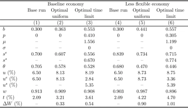
Table 1. Numerical results without monitoring and sanctions.
Baseline economy Less ‡exible economy Base run Optimal Optimal time Base run Optimal Optimal time
uniform limit uniform limit
(1) (2) (3) (4) (5) (6) b 0.300 0.363 0.553 0.300 0.441 0.557 p 0 0 0.410 0 0 0.305 ¹ – – 1.556 – – 1.199 ¾ – – 0 – – 0 se 0.700 0.607 0.556 0.839 0.734 0.715 ss – – 0.670 – – 0.774 µ 0.705 0.578 0.528 0.680 0.470 0.446 u (%) 6.50 8.13 8.19 6.50 8.73 8.75 ue (%) 6.50 8.13 2.84 6.50 8.73 3.36 us (%) – – 5.35 – – 5.39 w 0.913 0.909 0.908 0.903 0.987 0.896 t (%) 2.09 3.21 3.61 2.09 4.22 4.70 ¢W (%) – 0.33 0.54 – 0.90 1.01
The last line of Table 1 presents welfare gains associated with particular policies. The welfare gain has the interpretation of a “consumption tax” (in percent) that equalizes the welfare across two policy regimes. To be speci…c, let WR represent welfare associated with the base run and WA
welfare associated with an alternative policy. Our measure of the welfare gain of policy A relative to policy R is given by the value of the tax rate ¿
that solves WA[(1¡¿)m;¢] = WR. With logarithmic utility functions we have ¢W ´ WA
¡WR =
¡ln(1¡¿) ¼ ¿. The welfare gains are always reported relative to the base run. In order to compare, say, the system with time limits with the optimal uniform system, one only has to take the di¤erence between the two entries for the welfare gain (¢W).
In columns 2 and 5 of Table 1, we report the results of determining the op-timal uniform replacement rate. The opop-timal replacement rate in the baseline economy is around 36 percent. A higher replacement rate reduces search in-centives and inin-centives for wage restraint, so unemployment increases. With the optimal uniform replacement rate, unemployment rises to reach 8.1 per-cent. Individuals living in the baseline economy would be willing to pay 0.33 percent of consumption to move from a replacement rate of 30 percent to an optimal uniform one. The optimal uniform replacement rate in the “less
‡exible” economy is higher since the cost of raising the replacement rate in terms of reducing search incentives is lower. The replacement rate equals 44 percent in the less ‡exible economy and unemployment increases to 8.7 percent. Individuals in the less ‡exible economy would be willing to pay 0.9 percent of consumption in order to live in the optimal uniform system.9
The characteristics of the optimal system with time limits are given in column 3 and 6. In the baseline economy, bene…t di¤erentiation is substantial and the duration of UI bene…t receipt is fairly short – the value of¹translates to an expected duration of around two months. The UI replacement rate amounts to 55 percent of the wage; the penalty associated with the loss of entitlement is around 41 percent. The bene…t system with limited duration is substantially more generous than the system with in…nite duration; with …nite duration, unemployment expenditure per non-employed equals 40.5 percent. When search is less elastic, the UI replacement rate is about the same (58 percent) as in our base case. However, the penalty associated with loosing entitlement is decidedly smaller (31 percent), and the expected duration of UI receipt is longer (around 11 weeks). The unemployment rate is only marginally higher than in the uniform system.
Because the government has two additional instruments (¹andp) besides
b it is not surprising that the welfare gain in the exogenous time limit case exceeds the welfare gain in the optimal uniform case in both economies. The relative gain of introducing time limits is, however, smaller in the less ‡exible economy than in the baseline economy. Also note that unemployment goes up by moving from the optimal uniform system to exogenous time limits. In other words, unemployment is not a su¢cient statistic for welfare in this case.
4.2
Monitoring and Sanctions
This section has three purposes. First, we consider the trade-o¤ between monitoring and punishment, i.e., we want to examine whether the Beckerian prescription regarding optimal crime deterrence will be an outcome of the model. Second, we evaluate the case for monitoring and calculate the optimal monitoring and sanctions system (if it exists). Third, we investigate whether the penalties and sanctioning rates generated by the model are in broad
9Notice that one should not compare the values of the consumption taxes across the
conformity with the data.
4.2.1 The Trade-o¤ Between Monitoring and Sanctions
Our model features costly monitoring but, apart from the utility loss of those sanctioned, there is no cost associated with imposing the penalty. In this sense, the model …ts within the Beckerian framework of crime and pun-ishment; see Becker (1968). Becker’s celebrated paper suggested that opti-mal crime deterrence should involve maximum penalties with (close to) zero probability. Translated to our setting this prescription would suggest that maximum welfare is achieved at ¹! 0, p !1. Will be this be an outcome of our model?
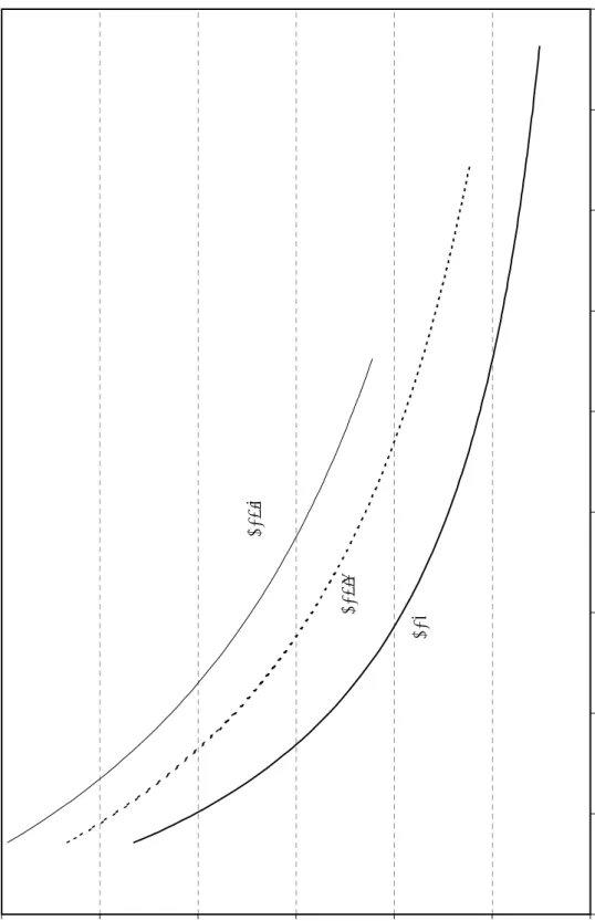
Assume thatc(¾)takes the form ofc(¾) =±¾. To illustrate the trade-o¤ between monitoring and punishment we vary the marginal cost of monitoring,
±, holding the UI replacement rate constant at b = 0:405, which equals the expenditure per non-employed implied by the optimal system with time limits. Each value of ± implies an optimal combination of the extent of monitoring (¹) and the size of the sanction (p). As ± becomes bigger, one would expect to approach the Becker solution with maximal penalty and minimal monitoring expenditure.
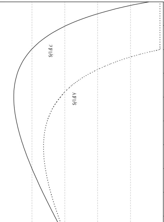
Figure 1 traces out the optimal combinations of¹andpfor di¤erent val-ues of ± (same curve) and three di¤erent values of ¾ (di¤erent curves). The optimal combination is never the Beckerian corner solution (¹!0, p!1). Before reaching the corner solution the social planner reverts back to the optimal uniform system. At this point we stop drawing the lines in Figure 1. So, for instance, the pointf¹= 0:05; p= 0:63gon the curve labeled “¾ = 1” represents the last point when the monitoring and sanctions system is oper-ative. Risk aversion in combination with a random monitoring technology implies that it is not optimal to impose the maximal sanction. The reason is that with risk aversion a sanction is no longer a costless transfer of money from the agent to the government. Relying on a maximal penalty to deter suboptimal search such that the penalty is never administered in equilibrium is also not an option in our case. Because we assume that the monitoring technology is imperfect, some agents will be penalized in equilibrium and, therefore, the monetary sanction should be …nite.
4.2.2 Are Monitoring and Sanctions Always Optimal?
The argument in favor of monitoring and sanctions hinges crucially on the costs of this system. Unfortunately, the cost associated with monitoring and sanctions is something of a black box. Therefore, we give an upper bound on the marginal cost below which monitoring and sanctions are an ingredient of the optimal system. Since this upper bound turns out to be very high, we go on to characterize the optimal UI system with monitoring and sanctions. Is it optimal to introduce monitoring and sanctions? In proposition 2 we stated the condition when the introduction of monitoring and sanctions represents a welfare improvement. For the introduction of monitoring and sanctions to be a welfare improvement relative to the case with time limits,
c0(0)has to be less than the gain as represented by greater search incentives among UI recipients with monitoring. We have calculated the cut-o¤ value for our two economies. In our base case, this cut-o¤ value (^c) equals ^c= 0:076; in the alternative case, we have ^c= 0:047. Both of these numbers have to be considered extremely high. Since the marginal product of labor and the labor force are normalized to unity, we can relate these cut-o¤ values to (private sector) GDP by dividing by the employment rate (which is around 92 percent in the optimal system with time limits). So, the calculated cut-o¤ values suggest that as long as the marginal cost is no greater than 4:7=0:92 = 5:1
(7:6=0:92 = 8:3) percent of GDP, it is optimal to introduce monitoring and sanctions. Since these numbers are very large, the introduction of monitoring and sanctions is most likely a welfare improvement relative to the case with time limits.
What is the optimal design of a monitoring and sanctions system? This clearly depends on the exact form of the cost functionc(¾). As above, we use the cost function c(¾) =±¾. To estimate a reasonable value for ±, we used Swedish data on the relative number of employees at the Public Employment Service (PES), since PES o¢cers are responsible for monitoring job search in Sweden. We also used information on how often each PES employee meets a particular unemployed, and the fraction of total time that the PES o¢cer spends in meetings with the unemployed. This calculation, which is presented in greater detail in Appendix B, suggests that the marginal cost of monitoring is in the order of c(¾) =±¾ = 0:00785. Provided that ¾ ¸0:785
in Sweden, then ± = 0:01 is a conservative estimate. We also conduct an alternative calculation where ± = 0:02. Note that in both cases ± < c^and hence monitoring and sanctions improve welfare.
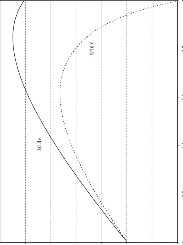
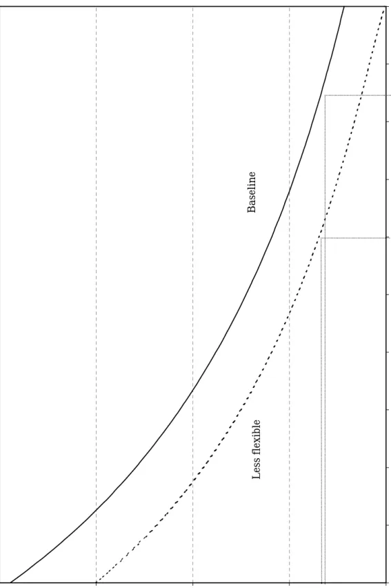
Figure 2 plots welfare against¾ for the base case with the two alternative values of ±. With ± = 0:01, the maximum is at ¾ = 0:85 and with± = 0:02
the principal chooses a less precise technology (¾ = 0:62). Figure 3 gives a similar plot, but this time for the less ‡exible economy. In the less ‡exible economy, agents’ search is less a¤ected by incentives. Thus, there is less scope for stimulating search via ¾. Hence, the principal opts for a less precise technology in this case.
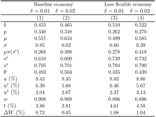
Table 2. Numerical results with monitoring and sanctions. Baseline economy Less ‡exible economy
± = 0:01 ±= 0:02 ±= 0:01 ±= 0:02 (1) (2) (3) (4) b 0.455 0.465 0.510 0.522 p 0.340 0.348 0.262 0.270 ¹ 0.557 0.634 0.499 0.585 ¾ 0.85 0.62 0.60 0.39 ¹¼(se) 0.268 0.398 0.278 0.418 se 0.610 0.600 0.739 0.732 ss 0.705 0.701 0.794 0.790 µ 0.493 0.504 0.435 0.439 u (%) 8.43 8.35 8.83 8.80 ue (%) 6.39 5.68 6.46 5.67 us (%) 2.04 2.67 2.37 3.13 w 0.908 0.908 0.896 0.896 t (%) 3.88 3.81 4.61 4.58 ¢W (%) 0.72 0.65 1.08 1.04
Table 2 presents some numbers that correspond to the optimal systems in each economy for the two values of±. Note that even for±= 0:02, the optimal
¾ is strictly positive and welfare is higher than in Table 1 for both economies. Again, the relative gain of designing an optimal system with monitoring and sanction is greater in the baseline economy. In the less ‡exible economy, the bulk of the total gain stems from introducing an optimal uniform system; cf. Table 1. In the baseline economy, on the other hand, the relative gains are more evenly spread out over the institutional changes of the UI system. Also note that both economies experience a rise in unemployment as compared to Table 1 although the additional instrument does raise welfare. Finally,
note that the fraction of unemployed with a sanction is considerably lower in Table 2 than in the columns with exogenous time limits in Table 1. Less people need to be penalized in a monitoring system in order to get similar welfare and search incentive e¤ects.
4.2.3 A Brief Look at the Data
Having calculated the optimal systems with monitoring and sanctions it is tempting to relate the predictions of the model to the data. Some of the pa-rameters of the monitoring and sanctions system are of course unobservable. However, there are observations on the UI replacement rates, the penalties for violating search requirements, and the associated sanctioning rates. Pre-sumably, there is a lot of noise in the data pertaining to sanction rates. Nevertheless, there is great variation in these data as is clear from Grubb (2001). It seems that the US and Switzerland are the extreme cases in terms of having systems with a large number of sanctions. In the US in the late 1990s, around 10 percent of bene…ciaries were sanctioned each quarter for be-havior during the bene…t period. In addition, some 25 percent of the (stock of) eligible unemployed were “sanctioned” because they exhausted their ben-e…ts.10 Based on these data, the quarterly sanction rate in the US would be in
the order of 35 percent. With the exception of Switzerland, sanctions during the bene…t period are substantially less common in the European countries; in fact, the sanction rates are typically lower than one percent per quarter. See Grubb (2001) for further details.
The number of sanctions seems to be inversely related to the severeness of the penalty. In the US, the normal sanction for a job search infringement is a loss of bene…ts for one week. In Sweden, on the other hand, the penalty until recently was the loss of bene…ts for twelve weeks.11 Thus, there seems
to be a trade-o¤ of the form implied by Figure 1 in the data.
What does the model have to say about the number of sanctions? Fig-ure 4 addresses this question by plotting the sanctioning rates for the two economies and ± = 0:01. Sanctioning rates decline in ¾ for two reasons: …rstly, for given se, a rise in¾ reduces¼(se) ;and, secondly, a rise in¾ raises
10This estimate is a crude average for the period 1995-2000. The number of exhaustions
per quarter amounted to some 600 000 individuals, the number of unemployed to 6.5 millions, and the fraction eligible for UI to 35 percent. Source: US Department of Labor (labor force statistics and UI program statistics).
se: In comparison to sanctioning data for the typical European country, the
model predicts that sanctioning rates are on the high side except for the less ‡exible economy with values of ¾ in excess of 0.90. However, such high values of ¾ are not optimal. With an optimal choice of the monitoring and sanctions system, the sanctioning rates are remarkably similar across the two economies: the number of sanctions hovers around 27 percent per quarter. Taken at face values, our models indicate that many countries do not have an optimal system of monitoring and sanctions. On the account of the sanction rate, however, our models …t well with the US data. For a lot of European countries the sanction rate seems to be far below the optimal rates.12
5
Concluding Remarks
In this paper we have analyzed the design of optimal unemployment insurance in a search equilibrium framework where search e¤ort among the unemployed is not perfectly observable. We have examined to what extent the optimal policy should involve monitoring of search e¤ort and bene…t sanctions if ob-served search is found insu¢cient. The results suggest that the introduction of a system with monitoring and sanctions represents a welfare improvement for reasonable values of the monitoring costs. Those costs would have to be implausibly high – higher than …ve percent of GDP – for this conclusion not to hold.
The policy prescription following from our analysis is thus di¤erent from Becker’s (1968) well known result, where the penalty should be maximal and the probability of getting caught should be close to zero. The key assumption delivering our results is that individuals are risk averse. With imperfect monitoring some individuals will be sanctioned in equilibrium and giving them the maximal one can never be optimal with risk aversion.
While we are reasonably comfortable in saying that monitoring and sanc-tions represent a welfare improvement, it is much more di¢cult to give clear advice on the characteristics of such a system. The reason for this conclusion is that the exact formulation of the monitoring and sanctions system depends
12We have also considered an alternative scenario of a “low turnover” economy that
has a lower job destruction rate Á and higher value for a in the matching function to
keep unemployment at the baseline value of 6.5 percent. The UI replacement rate and the penalty are more or less identical to the baseline economy. However, the optimal number
on the cost of running such a system. Unfortunately, the cost of running the system is something of a black box.
An issue that we have not addressed is the possibility that formal search requirements may induce individuals to use formal rather than informal search methods and therefore bring little increase in total search intensity. Nevertheless, it is likely thatgeneral search requirements – such as the num-ber of job applications …led during a week – should minimize the risk of substitution between search channels. Presumably, substitution is going to be more severe in systems where search requirements are linked to formal channels such as referrals by the public employment service. On this ac-count, therefore, search requirements speci…ed in terms of independent job search, as used in the US, the Netherlands and Switzerland, seem to be preferable.
Appendix A: The Sanctioning Probability
This appendix addresses the “structural” interpretation of our sanction-ing probability: ¼(se) = 1¡¾se. In order to motivate this speci…cation, we have to introduce some variation in search, either across individuals or across time. Suppose, then, that individuals make random optimization errors such that actual search (se
a) varies randomly around the privately optimal level
(se): se
a=se+», whereE(») = 0. One story motivating this kind of
speci…-cation is that individuals make the right choices in steady state, but outside steady state there may be some random departures from optimality. Another interpretation, that strictly does not …t with our homogeneity assumption, is that there is some, but unimportant, heterogeneity among individuals.
Suppose, realistically, that bene…t administrators observe actual search with error. Conditional on se
a units of search, observed search can be
de-composed into a systematic part and an idiosyncratic part that varies across administrators, i.e. seobs = (1¡¾)s+¾sea+", where s denotes the mean of
the distribution, i.e. s¹=E(seobs) =E(sea), and E(") = 0:
A useful way to think about the systematic part is that it has been determined by linear projection. So, once upon a time the national ben-e…t administrations o¢ce collected data on some indicator of search, such as the number of …led job applications, and observed search. If se
obs =
sea+º, then E(seobsjs e
a) = (1¡¾)s+¾sea, where s = E(seobs) = E(s e
a) and
¾ = 1. With an observation technology that has no informational content
(var(sea)=var(º)) = 0 and ¾ = 0; based on the projection, one would then
infer that a particular individual searches like the average individual in the population. Therefore, we think of the parameter ¾ 2 [0;1] as indexing the precision of the inspection technology.
There is also variation in “inferred search” depending on the inspect-ing bene…t administrator ("). Let R denote the search requirement. Then the worker is sanctioned whenever: seobs · R. The probability of being sanctioned, given that the worker supplies se
a = se equals ¼(se) = Pr(" ·
R¡(1¡¾)¹s¡¾se) = F (R
¡(1¡¾)¹s¡¾se), where F(
¢) denotes the dis-tribution function. Let us make the simplifying assumptions that F(¢) is symmetric and uniform with unit density. Under these conditions we have
" 2(¡0:5;0:5) and the probability of being sanctioned can be written as
¼(se) = 1¡
Z (1¡¾)¹s+¾se¡R
¡0:5
d"= 1¡¾se+ (R¡0:5¡(1¡¾)¹s)
Now, we want to make sure that ¼(¢) is a proper probability. To do this, we set R= 0:5 + (1¡¾)¹s somewhat arbitrarily. Hence, we get¼(se) = 1
¡¾se.
Since ¾ 2[0;1] andse
2[0;1], we have ¼(se)
2[0;1]. With this assumption, we are implicitly changing the search requirement when we change the value of ¾. Part of the reason for making this assumption is of course simplicity. Another justi…cation is that our model feaures no costs of changing the search requirement. A satisfactory treatment of search requirements requires that these costs are appropriately speci…ed.
Appendix B: Estimating the Marginal Cost of Monitoring To obtain a reasonable value for the cost of monitoring an additional indi-vidual (c(¾)) we performed the following calculation. We relied on data from Sweden, where PES administrators are responsible for monitoring whether unemployed individuals have searched to rule or not. Three sources of infor-mation were used: (i) the relative number of employees at the PES; (ii) the fraction of time that a PES o¢cer meets with the unemployed; and (iii) the number of contacts between the PES o¢cer and a particular unemployed in-dividual. Information pertaining to items (ii) and (iii) is taken from Lundin (2000).
In the main text the total cost of the monitoring and sanctions system was speci…ed as: C =c(¾)¹uew. To get an approximate value for C we start
be calculating the wage bill paid to individuals involved in monitoring. Since the labor force and the marginal product of labor are normalized to unity, the wage bill is measured relative to these items. The PES service employs approximately 10,000 individuals in Sweden, which translates to around 0.25 percent of the labor force. On average PES o¢cers spend 30 percent of their time in meetings with the unemployed. Assuming that the unemployed are monitored each time they meet with a PES o¢cer we have C = 0:0025£ 0:3w= 0:00075w. Thus we have C =c(¾)¹uew= 0:00075w. Turning to the left-hand side of this equation, we set the number of unemployed individuals eligible for UI to 5 percent. With this assumption, we only need an estimate of¹to get an estimate ofc(¾). The information used to estimate¹is derived from a question put to PES o¢cers regarding the number of meetings with individuals searching for a job. When asked about there contact frequency, 35 percent of PES o¢cers answered “at most once a month”; 34 percent answered “at most once every other month”; and 31 percent answered “at most once every quarter”. Thus on average a PES o¢cer have (1£0:35 + 0:5£0:34 + 0:31=3)£3 = 1:91 meetings with a particular unemployed per quarter. Hence we have c(¾) = 0:00075=(¹ue) = 0:00075=(1:91
£0:05) ¼
0:00785. There is still one unknown in this equation, however; the estimated value of c(¾) pertains to a given value of ¾. Assuming that c(¾) = ±¾, we have ± = 0:01 for ¾ = 0:785 and ± = 0:02 for ¾ = 0:785=2. What is a reasonable estimate of ¾ for the Swedish case? With the structural interpretation of the sanctioning probability given above, we can transform these values into correlations between actual and observed search. Given the above interpretation of¾, the correlation between actual and inferred search is simply the square root of ¾. Therefore, if this correlation is greater than
(0:785)0:5
¼ 0:886, then ± = 0:01 is a conservative number. Alternatively, if this correlation is greater than (0:785=2)0:5
¼ 0:626, then ± = 0:02 is a conservative estimate.
References
Abbring, J.H., G.J. van den Berg and J.C. van Ours (1997) The e¤ect of unemployment insurance sanctions on the transition rate from unem-ployment to emunem-ployment, Working Paper, Tinbergen Institute, Ams-terdam.
Becker, G. (1968) Crime and punishment: An economic approach, Journal of Political Economy, 76, 169-217.
Baily, M.N. (1978), Some aspects of optimal unemployment insurance, Jour-nal of Public Economics, 10, 379-402.
Benus, J., J. Joesch, T. Johnson and D. Klepinger (1997) Evaluation of the Maryland unemployment insurance work search demonstration: Final report, Batelle Memorial Institute in association with Abt Associates Inc (http://wdr.doleta.gov/owsdrr/98-2/).
Black, D., J. Smith, M. Berger and B. Noel (1999) Is the threat of training more e¤ective than training itself? Experimental evidence from the UI system, manuscript, Department of Economics, University of Western Ontario.
Boone, J. and J. van Ours (2000) Modeling …nancial incentives to get unem-ployed back to work, Discussion Paper 2000-02, CentER for Economic Research, Tilburg University.
Broersma, L. and J.C. van Ours (1999) Job searchers, job matches and the elasticity of matching, Labour Economics, 6, 77-93.
Cahuc, P. and E. Lehmann (2000) Should unemployment bene…ts decrease with the unemployment spell?, Journal of Public Economics, 77, 135-153.
Flemming, J.S. (1978) Aspects of optimal unemployment insurance: Search, leisure, and capital market imperfections,Journal of Public Economics, 10, 403-425.
Fredriksson, P. and B. Holmlund (2001) Optimal unemployment insurance in search equilibrium, Journal of Labor Economics, 19, 370-399.
Garoupa, N. (1997) The theory of optimal law enforcement, Journal of Economic Surveys, 11 267-295.
Grubb, D. (2001) Eligibility criteria for unemployment bene…ts, in Labour Market Policies and Public Employment Service, OECD.
Hopenhayn, H.A. and J.P. Nicolini (1997) Optimal unemployment insur-ance, Journal of Political Economy, 105, 412-438.
Hosios, A.J. (1990) On the e¢ciency of matching and related models of search and unemployment, Review of Economic Studies, 57, 279-298. Johnson, T. and D. Klepinger (1994) Experimental evidence on
unemploy-ment insurance work-search policies, Journal or Human Resources, 29, 695-717.
Lundin, M. (2000) Tillämpningen av arbetslöshetsförsäkringens regelverk vid arbetsförmedlingarna, stencil 2000:1, O¢ce of Labour Market Pol-icy Evaluation (IFAU), Uppsala.
Mortensen, D.T. (1977) Unemployment insurance and job search decisions,
Industrial and Labor Relations Review, 30, 505-517.
Pissarides, C.A. (1990)Equilibrium Unemployment Theory, Basil Blackwell, Oxford.
Polinsky, A.M. and S. Shavell (2000) The economic theory of public enforce-ment of law, Journal of Economic Literature, 38, 45-76.
OECD (2001)Labour Market Policies and Public Employment Service, Paris. Shavell, S. and L. Weiss (1979) The optimal payment of unemployment
insurance bene…ts over time, Journal of Political Economy, 87, 1347-1363.
Van den Berg, G.J., B. van der Klaauw and J.C. van Ours (1998) Punitive sanctions and the transition rate from welfare to work, Discussion Paper 9856, CentER for Economic Research, Tilburg University.
Van den Berg, G.J. and B. van der Klaauw (2000) Counseling and moni-toring of unemployed workers: Theory and evidence from a social ex-periment, manuscript, Free University of Amsterdam.
0.25 0.3 0.35 0.4 0.45 0.5 0.55 0.6 0.65 Sanction ( p ) Monitorin g ( µ ) σ= 1 σ= 0. 5 σ= 0. 1
0 0.2 0.4 0.6 0.8 1
Figure 2: Welfare as a function
σ
, baseline economy The
precision of the ins
pection technolo gy ( σ ) δ=0. 01 δ= 0. 02
0 0.1 0.2 0.3 0.4 0.5 0.6 0.7 0.8 0.9 1 Precision of ins pection technolo gy ( σ ) δ= 0. 01 δ= 0. 02 Fi
gure 3: Welfare as a function
σ
0 0.1 0.2 0.3 0.4 0.5 0.6 0.7 0.8 0.9 1 Fi gure 4: Q uarterl y sanction rates, δ =0.01
Precision of inspection technology (
σ
)
Baseline