The Effect of CASE Tools on Software Development Effort

ABSTRACT

CASE (Computer Aided Software Engineering) tools have played a critical role in improving software productivity and quality by assisting tasks in software development processes since 1970’s. Several parametric software cost models adopt “use of software tools” as one of environmental factors that affect software development productivity. However, most software development teams use CASE tools that are assembled over time and adopt new tools without establishing formal evaluation criteria. Several software cost models assess the productivity impacts of CASE tools based just on breadth of tool coverage without considering other productivity dimensions such as degree of integration, tool maturity, and user support. This paper provides an extended set of tool rating scales based on the completeness of tool coverage, the degree of tool integration, and tool maturity/ user support. It uses these scales to refine the way in which CASE tools are effectively evaluated within COCOMO (COnstructive COst MOdel) II. In order to find the best fit of weighting values for the extended set of tool rating scales in the extended research model, a Bayesian approach is adopted to combine two sources of (expert-judged and data-determined) information to increase prediction accuracy. The research model using the extended three TOOL rating scales is validated by using cross-validation methodologies such as data splitting and bootstraping.

Keywords

CASE (Computer Aided Software Engineering), Software tools, Software Productivity, Software Cost Models, Empirical Studies, Software Metrics

1 INTRODUCTION

It is said that an appropriate set of CASE tools can lead to the improvement of software productivity and quality by replacing human tasks with automated support in the software life-cycle. Most software development teams use a variety of CASE tools with the hope of improving productivity. However, the proliferation of CASE tools makes it difficult to evaluate currently used or newly adopted tools with effectiveness, even though several

sources[1][2] provide guidelines.

During the last two decades, software cost models have been developed to predict effort, schedule, and cost for the product being developed. Several of those models have employed “use of software tools” to assess the impacts on software development effort. While most of those software models are proprietary, COCOMO II is a fully documented and widely accepted model, updated from the original COCOMO and Ada COCOMO[3][4][5]. COCOMO II uses TOOL, one of the Effort Multipliers in its Post-Architecture model to capture the impacts on software productivity and provides a TOOL rating scale based just on the completeness of tool coverage as a guideline for the evaluation of software tools. This paper describes COCOMO II briefly and shows the productivity impact on project’s TOOL rating level, based on regression analysis of the COCOMO II database. However, even though the COCOMO II TOOL rating scale has been updated for 1990’s software tools from the original COCOMO TOOL rating scale, it may not be complete without considering other important factors such as degree of tool integration, tool maturity, and user support. Those factors are frequently used in many software evaluation criteria[2][6][7]. This paper provides a set of TOOL rating scales to reflect those important factors.

The latest version of COCOMO, calibrated with a Bayesian approach that combines expert-judged and data-determined information, has fairly good prediction rates that are within 20% of actuals 56% of the time, within 25% of actuals 65% of the time, and within 30% of actuals 71% of the time[8]. This research adopts the Bayesian modeling methodology to extend the COCOMO II Post-Architecture model with the extended set of TOOL rating scales. Also, this paper introduces cross-validation methods such as data-splitting and bootstrap that are widely used to check regression models.

2 COCOMO II AND PRODUCTIVITY IMPACT

COCOMO II has been updated from the original COCOMO [3] and its Ada successor [4] in order to address the issues on new process models and capabilities such as concurrent, iterative, and cyclic processes; rapid application development, COTS (Commercial-Off-The-Shelf) integration and software maturity initiatives. The COCOMO II research effort targets the estimation of software projects in the 1990’s and 2000’s. The definition and rationale are described in [5]. The initial definition of the model has been LEAVE BLANK THE LAST 2.5 cm (1”)

You can preserve this space with an

anchored frame (8.4 cm x 2.5 cm), anchored to the bottom of the column.

OF THE LEFT COLUMN ON THE FIRST PAGE FOR THE COPYRIGHT NOTICE.

The Effect of CASE Tools on Software Development Effort

Jongmoon Baik, Barry Boehm

Center for Software Engineering

Computer Science Deptartment

University of Southern California

Los Angeles, CA USA

+1 213 740 5703

{jobaik,boehm}@sunset.usc.edu

Bert Steece

Information and Operations Department

Marshall School of Business

University of Southern California

Los Angeles, CA USA

+1 213 740 0674

[email protected]

refined as actual project data points are collected and analyzed.

The COCOMO II provides a tailorable mix of three submodels: Application Composition Model, Early Design Model, and Post-Architecture Model. These are consistent with the granularity of the available information in a software development lifecycle in order to support software estimation. The Post-Architecture model estimates the effort and the schedule involved in the development and maintenance of a software product after the lifecycle architecture of the software product is established. It is the most mature model among the three models and has been calibrated for more accurate estimation. This section discusses the Post-Architecture Model and the analyzed result of the COCOMO II database focusing on the CASE tool productivity impact on software development effort within the model.

Post-Architecture Model

COCOMO II Post-Architecture model is the most mature and detailed model among the three models. It is best applied when the system architecture is developed. It predicts the development effort in PM (Person months), via the following equation.

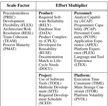
The key inputs of the model are Software Size, 5 Scale Factors and 17 Effort Multipliers (Cost Drivers). Those Scale Factors and Effort Multipliers are listed in Table 1. The exponent E in the above equation is an aggregation of five Scale Factors to capture the relative economies or diseconomies of scale encountered for software projects of different sizes[9].

If E = 1.0, the economies and diseconomies of scale are in balance.

If E > 1.0, the project exhibits diseconomies of scale. This is generally because of two main factors: growth of interpersonal communications overhead and growth of large-system integration overhead.

If E < 1.0, the project exhibits economies of scale.

The 17 Effort Multipliers are used in the model to adjust the nominal effort, PM, to reflect the software product under development. Each multiplicative Effort Multiplier is defined by a set of rating levels and a corresponding set of effort multipliers. The Nominal multiplier has the rating value of 1.0. Off-nominal values generally change the estimated effort. The detailed information about Scale

Factors and Multipliers is available in [5].

Productivity Impact in COCOMO II.2000

As mentioned earlier, COCOMO II.2000 was calibrated with 161 project data points by using a Bayesian approach that combines a priori (expert-judged) and sample (data-determined) information for the model parameters. The weighted values for the two sources of information to determine the posteriori distribution are assigned according to their variance (precision).That is, if the variance of a priori (expert) information is larger than that of the sample information, a higher weighted value is assigned to the sample information based on Bayes’ rule. Figure 1 shows how the posteriori productivity range (ratio between the least productive parameter rating and the most productive parameter rating) for TOOL rating is determined based on the precision of two information.

Figure 1. A-Posteriori update of COCOMO II TOOL Productivity Range

In this case, a higher weight is assigned to the lower-variance sample information causing the posterior mean to be closer to the sample mean. The t-value, 2.488, is the ratio between the estimate and corresponding standard error in the log-PM A (Size)E EM_i i=1 17

∏

∑

Where A = 2.94 and B = 0.91 (COCOMO II.2000)

Scale Factor Effort Multiplier

Precedentedness (PREC) Development Flexibility (FLEX) Architecture/Risk Resolution (RESL) Team Cohesion (TEAM) Process Maturity (PMAT) Product: Required Soft-ware Reliability (RELY) Database Size (DATA) Product Complex-ity (CPLX) Developed for Reusability (RUSE) Documentation Match to Life-Cycle Needs (DOCU) Personnel: Analyst Capabil-ity (ACAP) Programmer Capa-bility (PCAP) Personnel Conti-nuity (PCON) Application Expe-rience (APEX) Platform Experi-ence (PLEX) Language and Tool Experience (LTEX) Project: Use of Software Tools (TOOL) Multisite Develop-ment (SITE) Required Develop-ment Schedule (SCED) Platform: Execution Time Constraint (TIME) Main Storage Con-straint (STOR) Platform Volatility (PVOL)

Table 1: Scale Factors and Effort Multipliers

161 Projects

t = 2.488 Var.= 0.049

1.50 Bayesian A-posteriori

Var. =0.028 Expert Delphi_A-priori Var. = 0.167 1.0 1.25 1.5 1.75 2.0 1.92 1.43 161 Projects t = 2.488 Var.= 0.049 1.50 Bayesian A-posteriori

Var. =0.028 Expert Delphi_A-priori Var. = 0.167

1.0 1.25 1.5 1.75 2.0 1.92 1.43

transformed regression analysis for the 161 project data. It shows that the productivity range of TOOL has statistically a strong significance (t-value > 1.96) in estimating the software development effort. The practical interpretation of this result is that “increasing tool coverage makes a statistically significant difference in reducing software development effort, even after normalizing the effects of other variables such as process maturity. Given that previous anecdotal data still generates controversy on this point[10][11], this is a valuable result.

The productivity ranges for all parameters used in the COCOMO II Bayesian calibration is illustrated as the following.

Figure 2. Productivity Ranges for 5 Scale Factors and 17 Effort Multiplier in COCOMO II.2000

This figure delivers and overall perspective on the relative software productive ranges. The productivity range of the TOOL parameter shows a relatively high payoff in a software improvement activity.

3 MODELING APPROACH

This research uses the 7-step COCOMO II modeling methodology shown in Figure 3. It has been used to develop COCOMO II and other related models like COQUALMO (COnstructive QUALity MOdel)[5].

Step 1: Analyze literature for factors affecting the quantities

to be estimated.

The first step in developing a software estimation model is in determining the factors (or predictor variables) that affect the software attribute (or the response variable) being estimated. This was done by reviewing existing literature and analyzing the influence of software tools on development effort. The analysis led to the determination of three relatively orthogonal and potentially significant factors: tool coverage, integration, and maturity/support.

Step 2: Perform behavioral analyses to determine the effect

of factor levels on the quantities to be estimated.

This showed the behavioral effects of higher vs. lower levels of each factors on project activity levels.

Step 3: Identify the relative significance of the factors on the

quantities to be estimated.

After a thorough behavioral analyses was done, the relative significance and orthogonality of each tool factor was qualitatively confirmed, and rating scales were determined for each factor (Section 4). Also, a candidate functional form for a more robust COCOMO II TOOL parameter was determined. This is a weighted average of the three individual ratings:

Step 4: Perform expert-judgement Delphi assessment of the

model parameters; formulate a-priori version of the model. Here, cost estimation experts from among USC’s COCOMO II Affiliates were convened in a two-round Delphi exercise to determine a-priori values of the weights b₁, b₂, and b₃ (Section 5). This model version is based on expert-judgement and is not calibrated against actual project data. But it serves as a good starting point as it reflects the knowledge and experience of experts in the field.

Step 5: Gather project data and determine statistical

significance of the various parameters.

Fifteen out of 161 projects in the COCOMO II database were found to have valid rating levels for TCOV, TINT, and TMAT. Section 6 shows the resulting regression analysis.

Step 6: Determine a Bayesian A-Posteriori set of model

parameters.

Using the expert-determined drivers and their variances as a-priori values, we determined a Bayesian a-posteriori set of model parameters as a weighted average of the a-priori values and the data-determined values and variances, with weights determined by relative variances of the expert and data-based results (Section 7), including covariance effects.

Step 7: Gather more data to refine the model.

Continue to gather data, and refine the model to be increasingly data-determined vs. expert-determined.

1 1 . 5 2 2 . 5 C PL X AC AP PC AP T I ME PC ON R E L Y D O C U S I T E AE X P PV OL T O OL ST OR L T EX PMAT SC ED D A T A PE X P R E SL PR EC R U SE T E AM F L EX Pa r a m e te rs Productivity Range 1 1 . 5 2 2 . 5 C PL X AC AP PC AP T I ME PC ON R E L Y D O C U S I T E AE X P PV OL T O OL ST OR L T EX PMAT SC ED D A T A PE X P R E SL PR EC R U SE T E AM F L EX Pa r a m e te rs 1 1 . 5 2 2 . 5 C PL X AC AP PC AP T I ME PC ON R E L Y D O C U S I T E AE X P PV OL T O OL ST OR L T EX PMAT SC ED D A T A PE X P R E SL PR EC R U SE T E AM F L EX Pa r a m e te rs Productivity Range

Figure 3. COCOMO II 7-Step Modeling Methodology PRIOR

+ SAMPLE

= POSTRIOR

TOOL = b₁TCOV+b₂TINT+b₃T MAT b₁, ,b₂ b₃≥0

We are gathering TCOV, TINT, and TMAT ratings on future projects entered into the COCOMO II database.

4 TOOL RATING SCALES

Completeness of Tool Coverage (TCOV)

It is not an easy task to classify CASE tools by their functionalities that support specific tasks in the development process, since a large number of features are offered by current CASE technology[12]. However, it is necessary to partition the same kinds of tools by their functionalities to explain differences in productivity impact. This section provides an extension of the COCOMO TOOL rating scale with currently available CASE tools in the software market.

Figure 4. Tool Use Characteristics at CMM Levels

Some relationships have been established between tool functionality and the needs of a particular level of the Capability Maturity Model[13][14]. Figure 4 shows the view of the CASE technology/process relationship. The SEI CMM lists the provision of appropriate resources (including tool support) as a key consideration in maturity levels 2 to 5. Table 2 provides a classification of currently available tool sets based on how completely they support the given activities in the software process. Like the COCOMO TOOL rating scale, it also requires a certain amount of judgement to determine an equivalent tool support leve

l.

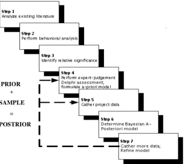
Degree of Tool Integration (TINT)

In a software process lifecycle, each individual tool promises higher quality and greater productivity. However, this promise has not been well realized since tool creators heven’t overcome the difficulties associated with integrating tools in an environment [15]. The main goals of integrating tools are concurrent data sharing and software reuse in a software development lifecycle. If tools are integrated effectively without perturbing other tools in an environment, several benefits such as the reduction of training costs and reduced software rework can be obtained [7]. Thereby, effort and schedule for the software development can be decreased. Table 3 shows another dimension of the CASE tool rating scale to evaluate how well tools are integrated and what kind of mechanisms are provided to exchange information

Rating TCOV

Very Low Text-Based Editor, Basic 3GL Compiler, Basic library Aids, Basic Text-based Debugger, Basic Linker

Low Graphical Interactive Editor, Simple Design Language, Simple Programming Support Library, Simple Metrics/Analysis Tool

Table 2: Rating Scales for Completeness of Tool Coverage

Nominal Local Syntax Checking Editor, Standard Template Support Document Generator, Simple Design Tools,

Simple Stand-alone Configuration Man-agement Tool, Standard Data Transforma-tion Tool, Standard Support Metrics Aids with Repository, Simple Repository, Basic Test Case Analyzer

High Local Semantics Checking Editor, Auto-matic Document Generator, Requirement Specification Aids and Analyzer, Extended Design Tools, Automatic Code Generator from Detailed Design, Centralized Config-uration Management Tool, Process Man-agement Aids, Partially Associative Repository (Simple Data Model Support), Test Case Analyzer with Spec. Verification Aids, Basic Reengineering & Reverse Engineering Tool

Very High Global Semantics Checking Editor, Tailor-able Automatic Document Generator, Requirement Specification Aids and Ana-lyzer with Tracking Capability, Extended Design Tools with Model Verifier, Code Generator with Basic Round-Trip Capabil-ity, Extended Static Analysis Tool, Basic Associative, Active Repository (Complex Data Model Support), Heterogeneous N/W Support Distributed Configuration Man-agement Tool, Test Case Analyzer with Testing Process Manager, Test Oracle Sup-port, Extended Reengineering & Reverse Engineering Tools

Extra High Groupware systems, Distributed Asyn-chronous Requirement Negotiation and Trade-off tools, Code Generator with Extended Round-Trip Capability,

Extended Associative, Active Repository, Spec-based Static and Dynamic Analyzers Pro-active Project decision Assistance

Rating TCOV

Table 2: Rating Scales for Completeness of Tool Coverage

between tools in an integrated environment. This classification is based on Wasserman’s five level model for integration of tools in software engineering environments [16]. Those five models are:

• Platform Integration: Tools run on the same hardware/ operating system platform.

• Data Integration: Tools operate using the shared data model.

• Presentation Integration: Tools offer a common user interface.

• Control Integration: Tools may activate and control the operation of other tools.

• Process Integration: Tool usage is guided by an explicit process model and associated process engine.

This rating scale classifies CASE tools in the scale, ranging from Very Low to Extra High, according to how well they support the above five integration models. It provides a set of mechanisms at each level to integrate tools in a development environment. If a different set of mechanisms are used, some amount of judgment is required to fit it to an equivalent level of degree of integration.

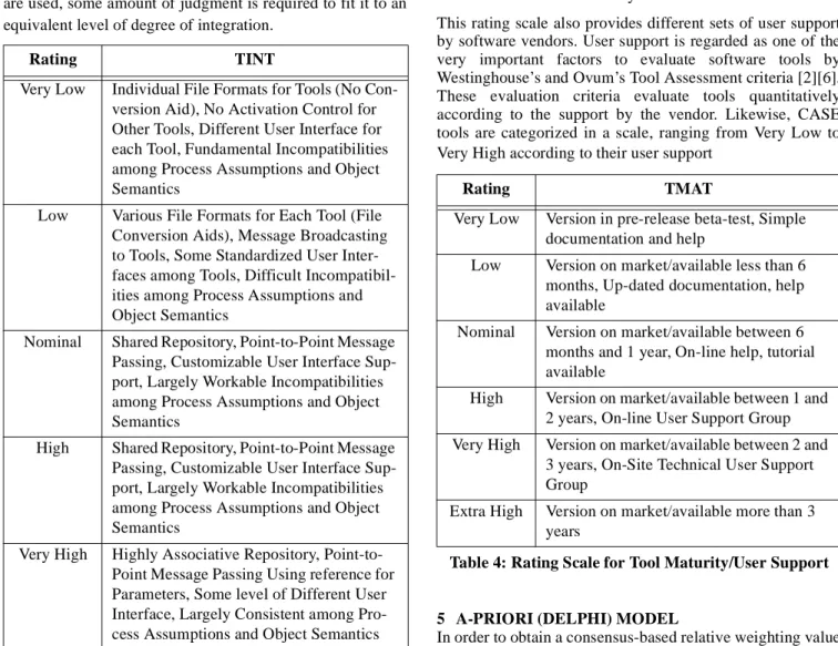
Tool Maturity/User Support (TMAT)

It is very difficult to verify how mature an adopted tool set is for software development. A general way to measure tool maturity is to see how long tools are used in the CASE tool market. As mentioned earlier, the maturity of software tools has a nontrivial effect on software quality and productivity. More errors are likely to be introduced during the development with a less mature tool, and consequently the more effort is required to correct those errors. Table 4 categorizes CASE tools according to the survival length in the software market after they are released.

This rating scale also provides different sets of user support by software vendors. User support is regarded as one of the very important factors to evaluate software tools by Westinghouse’s and Ovum’s Tool Assessment criteria [2][6]. These evaluation criteria evaluate tools quantitatively according to the support by the vendor. Likewise, CASE tools are categorized in a scale, ranging from Very Low to Very High according to their user support

5 A-PRIORI (DELPHI) MODEL

In order to obtain a consensus-based relative weighting value for each of the extended three TOOL rating scales, two rounds of Delphi analyses were carried out. This Delphi process gives an opportunity to apply the knowledge and

Rating TINT

Very Low Individual File Formats for Tools (No Con-version Aid), No Activation Control for Other Tools, Different User Interface for each Tool, Fundamental Incompatibilities among Process Assumptions and Object Semantics

Low Various File Formats for Each Tool (File Conversion Aids), Message Broadcasting to Tools, Some Standardized User Inter-faces among Tools, Difficult Incompatibil-ities among Process Assumptions and Object Semantics

Nominal Shared Repository, Point-to-Point Message Passing, Customizable User Interface Sup-port, Largely Workable Incompatibilities among Process Assumptions and Object Semantics

High Shared Repository, Point-to-Point Message Passing, Customizable User Interface Sup-port, Largely Workable Incompatibilities among Process Assumptions and Object Semantics

Very High Highly Associative Repository, Point-to-Point Message Passing Using reference for Parameters, Some level of Different User Interface, Largely Consistent among Pro-cess Assumptions and Object Semantics

Extra High Distributed-Associative Repository, Extended Point-to-Point Message Passing for Tool Activation, Complete Set of User Interface for Different Level of Users, Fully Consistent among Process Assump-tions and Object Semantics

Rating TMAT

Very Low Version in pre-release beta-test, Simple documentation and help

Low Version on market/available less than 6 months, Up-dated documentation, help available

Nominal Version on market/available between 6 months and 1 year, On-line help, tutorial available

High Version on market/available between 1 and 2 years, On-line User Support Group Very High Version on market/available between 2 and

3 years, On-Site Technical User Support Group

Extra High Version on market/available more than 3 years

Table 4: Rating Scale for Tool Maturity/User Support

Rating TINT

experience of experts in the field to the initial model. For this Delphi process, participants were selected from the COCOMO II affiliates: Commercial, Aerospace, Government, and nonprofit organizations. The steps taken for the 2-round Delphi process are described below.

First Round:

1. Provide participants with Delphi Questionnaire without initial weighting values

2. Collect responses

3. Ensure validity of responses by correspondence 4. Simple analysis of the responses

Second Round:

1. Provide participants with Delphi Questionnaire with the result of the first round

2. Repeat the above steps (2, 3, and 4) 3. Converge to Final Delphi results

Table 5 shows the results of the two round Delphi processes.

As shown in the above table, the participants agreed that the most productivity gains can be obtained via the higher tool ratings in TCOV with 47%. Even though differences in productivity gains in TINT and TMAT are 26% and 27% respectively, the variance of TINT is much smaller than that of TMAT.

6 SAMPLE (REGRESSION) MODEL

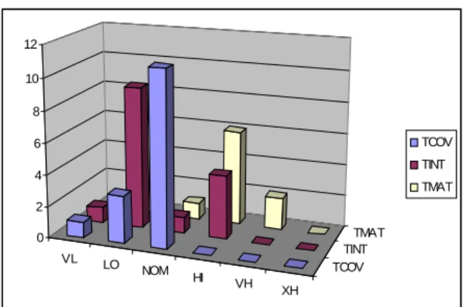
In order to find out the sampling information on the weighting value of three tool rating scales, 15 project data that have information about TCOV (Completeness of Activity Coverage), TINT (Degree of Tool Integration), and TMAT (Tool Maturity and User Support) were available from the COCOMO 81 database[3]. The TCOV ratings in the above table are the same as those in the original COCOMO 81 TOOL ratings. Since the data from 15 projects came from 1970’s and 1980’s, all cost drivers are displaced 2 places upward from COCOMO 81 to COCOMO II. Figure 5 shows the distributions of the ratings of data from the 15

projects based on the three dimensional TOOL rating scales.

Figure 5. Distribution of TCOV, TINT, and TMAT

In order to determine relative weighting values for TCOV, TINT, and TMAT, the following regression model was used to calculate the TOOL rating scales within COCOMO II.

again with the b_i non-negative and summing to 1.

Linear regression with the data from the 15 projects by Arc [18] gives the following results:

In the above regression result, Estimates are the estimated coefficients for the weighting values of b₁, b_{2 ,}and b₃, respectively. The Std. Error is the estimated standard deviation for each coefficient. The t-value is the ratio of residual error and variance for each predictor variable in the regression model and may be interpreted as the signal-to-noise ratio with the corresponding predictor variables. Hence, the higher the t-value, the higher the signal being sent by the predictor variable. In the Summary Analysis of Variance Table, the RSS (Residual Sum of Squares) is 0.027895 with 12 degrees of freedom. The sum of the estimated coefficients is not 1. Therefore, those values can

TCOV TINT TMAT

Mean 0.47 0.26 0.27

Variance 0.025694 0.005485 0.016875

Table 5:A-Priori Weighing Mean and Variance

Data set = TOOL_15_data, Name of Fit = L1 Normal Regression

Kernel mean function = Identity Response = TOOL

Terms = (TCOV TINT TMAT) With no intercept.

Coefficient Estimates

Label Estimate Std. Error t-value TCOV 0.515982 0.0888635 5.806 TINT 0.282561 0.107657 2.625 TMAT 0.165480 0.111398 1.485 Sigma hat: 0.048214 Number of cases: 15 Degrees of freedom: 12

Summary Analysis of Variance Table

Source df SS MS F p-value Regression 3 20.5056 6.8352 2940.40 0.0000 Residual 12 0.027895 0.00232459 VL _LO NOM _HI VH _XH TCOV TINT TMAT 0 2 4 6 8 10 12 TCOV TINT TMAT

be normalized as follows.

7 BAYESIAN CALIBRATION Bayesian Analysis

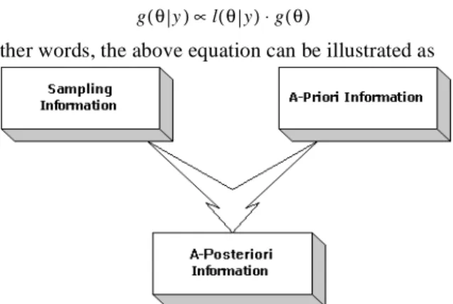
Bayesian inference is a statistical method by which similar information is combined to produce a posterior probability distribution of one or more parameters of interest. In Bayesian analysis, probability is defined in terms of a degree of belief and an estimator is chosen in order to minimize expected loss where the expectation is taken with respect to the posterior distribution of unknown parameters [17]. The procedure that combines a prior (expert-judged) information with sample information about the parameters of interest to produce a posterior probability distribution is done by using Bayes’ theorem as follows:

In the above equation, f denotes a density function for y and g denotes a density function for the unknown parameter vector b. f(y|q) is the joint density function which is algebraically identical to the likelihood function for q and contains all the sample information about unknown parameter q. g(q) is the prior distribution function for q summarizing non-sample information about q. The posterior distribution function, g(q|y), for q summarizes all information about q. With respect to q, f(y) can be regarded as a constant and f(y|q) can be written as the likelihood function l(q|y), then Bayesian theorem can be rewritten as follows:

In other words, the above equation can be illustrated as

Figure 6. Combination of Two Sources of Information A-Posteriori Model

In order to perform Bayesian analysis on the regression model, A-priori and small sample information is explained in the previous sections. The posterior mean and variance for

the unknown parameters b(or b**) and d (or Var(b**)) are defined as follows [19]:

where X is a matrix of observations on predictor variables, s is the variance of the residual for the sample data, and b* and

H* are the mean of prior information and the inverse of variance matrix, respectively. The posterior mean b** can be regarded as a matrix average of the prior and sample mean with weight s given by the precisions of all information about the unknown parameters. In other words, if the precision of the prior information is greater than that of the sample information, the posterior values will be closer to the prior values.

The derived posterior result for unknown parameters, coefficients and variances is summarized in Table 6. By combining two sources of information on parameters, the posterior variance gets smaller than those of the prior and sample.

As shown in the above table, the sum of posterior means for the weighting values of the extended three TOOL rating scales is not 1. Therefore, TOOL rating value in the research model can be determined by using normalized posterior coefficient means as follows:

This indicates that differences in tool coverage are the most important determinant of tool productivity gains, with a relative weight of 51%. The next most important is tool integration, with a relative weight of 27%. Tool maturity has the smallest effect but is still significant at a 22% relative weight.

Prediction Accuracy

The posterior model is calibrated with the data from the 15 projects to determine the best-fit relative weighting values for the three TOOL rating scales. In order to compare the model with the COCOMO II Bayesian estimation result, an evaluation criterion, the percentage of predictions that fall within X% of the actuals denoted as PRED(X), is used. The models are evaluated at PRED(.10), which is done by counting the number of MRE (Magnitude of Relative Errors)s [20] in the below less than or equal to 0.10 and dividing by the number of projects. The MRE for each TOOL = 0.54 TINT⋅ +0.29 TMAT⋅ +0.17 TCOV⋅

g(θ y) f y( θ)⋅g( )θ f y( )

---=

where

q: the vector of parameters of interest y: the vector of sample observations

g(θ y)∝l(θ y)⋅g( )θ

b₁ b₂ b₃

Mean 0.495104 0.259691 0.211617

Variance 0.00461028 0.00335019 0.00525464

Table 6: Posterior Weighting Mean and Variance

1 * 2 * *

]

1

[

)

b

(

=

X

′

X

+

H

s

Var

]

b

b

1

[

]

1

[

b

H

X

X

H

X

X

′

+

×

′

+

=

s

s

project is defined as the absolute value of the difference between the estimated project effort, E(Y) and actual project effort, Y, relative to the magnitude of the actual effort.

Table 7 summarizes the prediction accuracies of COCOMO II, sample without prior information, and posterior with prior information. Even though the prediction accuracies of sample and posterior estimates are the same (87%), the variances of the posterior coefficient estimates are smaller than those of sample regression model as shown earlier. Both the sample and posterior model give better prediction accuracies than the COCOMO II Bayesian model does because of the use of the 3 dimensional TOOL rating scales.

8 CROSS VALIDATION

There are several cross-validation techniques such as K-fold, Leave-one-out, Jackknife, Delete-d, and Bootstrap for regression problems [21]. In this chapter, two cross-validation methodologies supported by the program Arc are described. It also show the simulation results with COCOMO II 161 project data used for the calibration of the COCOMO II.2000 [5] (with one-dimensional TOOL and with the extended three dimensional TCOV, TINT, and TMAT) to validate the research model.

Cross-Validation by Data-Splitting

Cross-Validation by data-splitting is a widely-used model checking method to validate a regression model. This method randomly divides the original dataset into two subsamples - the first subsample (Construction, Model-building, or Training subsample) for exploration and model formulation, the second (Validation or Prediction subsample) for model validation, formal estimation, and testing [22]. Although the most ideal validation method is through the collection of new data, it is very hard to get new data in practice. So, data splitting is an attempt to simulate replication of the study.

In order to validate the model, we used the Arc statistical analysis program on two datasets of the same size (161 project data). For the TOOL rating value of the first dataset, the standard COCOMO II one dimensional TOOL rating scale was used. The TOOL rating value of the 15 projects with TCOV, TINT, and TMAT ratings was determined by the Bayesian weighted sum of the TCOV, TINT, and TMAT ratings. The TOOL ratings of the rest of the project data in the second dataset have the same values in the first dataset. For the two cross validations, we used the 115 project data points for the construction sets for the regression model

formation. The remaining 46 project data points were assigned into the validation datasets for regression model validation. Of those 15 projects, 11 were in the construction set and 4 were in the validation set.

In the above table, the output for the cross-validation in Arc includes a few summary statistics such as the weighted sum of squared deviations, mean of squared deviations, and a number of observations in the validation set. The sum of squared deviations (9.7475) with three dimensional TOOL validation set is a little bit smaller than the sum of squared deviations (9.76793) with the one dimensional TOOL validation set. The PRESS, predicted residual sum of squares, (0.260493) from the validation dataset with the extended TOOL rating scales is also smaller than the PRESS (0.262203) from the validation dataset with the one dimensional TOOL rating scale. The differences are not great, as only 9% (15 of 161) project data points have different values. But, they indicate an improvement, and they indicate stability with respect to the other variables.

Bootstrap

The bootstrap is a statistical simulation methodology that resamples from the original data set [24]. This methodology has been used to solve two of the most important problems (the determination of an estimator for a particular parameter of interest and the evaluation of that estimator through estimates of the standard error of estimator and the determination of confidence intervals) in applied statistics. Because of its generality, it has been used in wider application areas such as nonlinear regression, logistics regression, spatial modeling, and so on.

Here is a formal definition of the bootstrap by Bradley Efron [25]: a sample that has n independent identically distributed random vectors X₁, X₂, X₃,..., X_n and a real-valued estimator q(X₁, X₂, X₃,..., X_n) (denoted by ), the COCOMO II Bayesian Sample Regression Bayesian Posterior

Rating Scale TOOL TCOV, TINT, & TMAT

PRED (.10) 67% 87% 87%

Table 7: Comparison of Prediction Accuracies MRE_i E Y( )i–Yi

Y_i

---= ₁st _{validation set (TOOL)}

Cross validation summary of cases not used to get estimates:

Sum of squared deviations: 9.76793 Mean squared deviation: 0.212346 Sqrt(mean squared deviation): 0.460811 Number of observations: 46

> (/ (sum (^ (/ (send L1 :residuals) (- 1 (send L1 :leverages))) 2)) (send L1 :num-included)) 0.262203

2nd validation set (TCOV, TINT, and TMAT)

Cross validation summary of cases not used to get estimates:

Sum of squared deviations: 9.7475 Mean squared deviation: 0.211902 Sqrt(mean squared deviation): 0.460328 Number of observations: 46

>(/ (sum (^ (/ (send L1 :residuals) (- 1 (send L1 :leverages))) 2)) (send L1 :num-included)) 0.260493

Table 8: Cross Validation Summary and PRESS

procedure for the bootstrap to assess the accuracy of is defined in terms of empirical distribution function F_n that assigns the same probability 1/n to each observed value of the random vectors X_i (i = 1, 2,..., n) and is the likelihood estimator of the distribution for the observations when no parametric assumption are made. The bootstrap estimates is denoted q* that contains information to be used in making inference from data. The bootstrap distribution for can be obtained by generating values by sampling independently with replacement from empirical distribution F_n. The bootstrap estimation of standard error (q*- ) is the standard deviation of the bootstrap distribution for . From the bootstrap sampling, a Monte Carlo approximation of the bootstrap estimates is obtained. The procedure is described below:

1. Generate a bootstrap sample of size n (where n is the original sample size) with replacement from the original distribution.

2. Compute q*, the value of obtained by using the bootstrap sample in place of the original sample.

3. Repeat steps 1 and 2, k times.

This provides a Monte Carlo approximation to the distribution of q*. The standard deviation of the Monte Carlo distribution of q* is the Monte Carlo approximation of the bootstrap estimate of the standard error for . As the number of times of repeating steps 1 and 2 gets larger, there is very little difference between the bootstrap estimator and the Monte Carlo approximation. The main idea of the boot strap is that the two distributions are expected to be nearly the same.

We used the bootstrap option in the Arc program[26] to run 1000-case bootstrap samples for both the one-dimensional and three-dimensional TOOL ratings, by randomly sampling with replacement from the 161 project data points.

Table 9 shows the standard error and bias estimates obtained from the two bootstrap objects. The standard error estimates compare with the usual estimates obtained from the usual estimates with the two datasets, respectively. Note that the usual nominal regression estimates of standard error are the ideal bootstrap estimates of standard error as the number of boots adjusted by ([n / (n - k)]1/2). The bootstrap estimates of bias can be calculated as shown in the below equation from the idea “ * is to as is to ”. Those bootstrap estimates of bias for all predictor variables in the regression are relatively small because the usual normal

regression estimates are unbiased.

When compared with the bootstrap estimates of standard error and bias for log[TOOL] obtained from the one-dimensional TOOL dataset, the bootstrap estimates of standard error are a little bit smaller. Also, the bias estimate is reasonably small. That is, the normal regression model with three-dimensional TOOL ratings is better fit to the observations in the second dataset. Again, the differences are not great, but the results are stable and in the right direction.

Table 10 shows the corresponding percentile bootstrap confidence intervals for the coefficient estimates of Effort Multipliers. The detailed information on the confidence intervals are available in [25]. The default level for the confidence intervals is 95%. In repeated datasets, the true population mean will be included in the 95% confidence intervals. When compared with the normal regression estimates from the two datasets, respectively, the percentile bootstrap confidence intervals indicates that the resampling results agree closely with those obtained from standard methods.

Once again, most of the percentile confidence intervals from the three dimensional TOOL data set are narrower than those obtained from the one-dimensional dataset. Especially, the confidence interval for the coefficient of log[TOOL] from the three-dimensional dataset has a smaller region than that from the one-dimensional dataset shown in Figure 7. That is, the extended three dimensional TOOL rating scales (TCOV,

θ

ˆ

θ

ˆ

–

θ

θ

ˆ

θ

ˆ

θ

ˆ

–

θ

θ

ˆ

θ

ˆ

B

→

∞

θ

ˆ

θ

ˆ

θ

ˆ

θ

One-Dimensional TOOL Three Dimensional TOOL Std-Error Bias Std-Error Bias

log[ACAP] log[AEXP] log[CPLX] . . log[STOR] log[TIME] log[TOOL] 0.300547 0.458397 0.214933 . . 0.969903 0.604294 0.392941 -0.015081 0.099686 -0.026814 . . 0.382749 -0.155874 0.030489 0.306939 0.408997 0.206705 . . 0.967008 0.585690 0.359567 -0.015901 0.106427 -0.032947 . . 0.438698 -0.192345 0.042730

Table 9. Bootstrap Standard Error and Bias

Coefficients One-Dimensional TOOL Three Dimensional TOOL

log[ACAP] log[AEXP] log[CPLX] . . log[STOR] log[TIME] log[TOOL] (0.434194 1.67577) (-0.689046 1.11136) (0.514885 1.34717) . . (0.048242 3.24556) (0.194714 2.47158) (0.184884 1.67873) (0.449679 1.64775) (-0.505828 1.0968) (0.530155 1.35197) . . (0.0102692 3.18507) (0.173605 2.36188) (0.340032 1.71783)

Table 10. Bootstrap Confidence Intervals

Where

: ith coefficient in the regression

*_{(.): the average of} *_’s

θˆ

i

θˆi θˆi

TINT, and TMAT) gives a better fit of regression estimates than the one-dimensional TOOL rating scale does.

Figure 7. Confidence Interval for log[TOOL] 9 CONCLUSION AND FUTURE WORK

In this paper, a set of multi dimensional CASE tool rating scales are defined, which extend the COCOMO II TOOL rating scale and reflect important CASE tool environmental factors that have an effect on software development effort such as the degree of tool integration, tool maturity, and user support. This extends the constructive nature of COCOMO II by providing guidelines to evaluate CASE tools more effectively than the current one-dimensional TOOL rating scale in COCOMO II, based just on the completeness of tool coverage. This paper also introduces a method to calibrate the individual contribution to a multi dimensional parameter set. To find a best fit of the weighting values for the extended three rating scales, we use the Bayesian approach to combine two sources of (expert-judged and data-determined) information. Thereby, the prediction accuracy is improved from 67% to 87% with PRED(.10) over 15 project data points. Two cross validation results adopted from Arc show that the regression fit with the three dimensional tool rating scales is somewhat better than with the one dimensional TOOL rating scale, and is stable with respect to the other COCOMO II parameters.

The particular values should be considered provisional, as they are based on only 15 data points with detailed TOOL component ratings. But, since the t-values from the regression are strong, and since the relative magnitudes of the values exhibit consistency between the expert-determined and data-expert-determined values, we find sufficient justification to add the TOOL component parameters to the COCOMO II model. We plan to refine the parameter values as more data is collected.

REFERENCES

1. Robert Firth et. al. “A Guide to the Classification and Assessment of Software Engineering Tools”, CMU/SEI-87-TR-10, Carnegie Mellon University, Pittsburgh, PA, 1987.

2. Vicky Mosley, “How to Assess Tools Efficiently and Quantitatively”, IEEE Software, May 1992

3. Barry W. Boehm, Software Engineering Economics, Prentice Hall, 1981.

4. Barry W. Boehm and Walker Royce, “Ada COCOMO and Ada Process Model”, Proceedings of 5th COCOMO User’s Group Meeting, Software Engineering Institute, Pittsburgh, PA, Nov 1989.

5. Barry Boehm et. al., Software Cost Estimation with COCOMO II, Prentice Hall, 2000.

6. Contents and Services, Ovum Ltd., UK, Jun 1995. 7. Ian Sommerville, Software Engineering, 5th Edition,

Addison-Wesley Pub Co.,1995.

8. Sunita Chulani, Barry Boehm, and Bert Steece, “Baye-sian Analysis of Empirical Software Engineering cost Models”, IEEE Transactions on Software Engineering, pp. 513-583, July-Aug 1999.

9. Banker R., Chang and C. Kemerer, “Evidence on Econo-mies of Scale in Software Development”, Information and Software Technology, 1994.

10. Terry Bollinger, “Building Tech-Savvy Organiztions”, IEEE Software, pp.73-75, July/August 2000.

11. Bill Curtis, “Building Accelerated Organizations”, IEEE Software, pp. 72-74, July/August 2000.

12. Report on Project Management and Software Cost Esti-mation Technologies, STSC-TR-012, System Technol-ogy Support Center, Apr 1995.

13. Paulk, M. C. et. al., Capability Maturity Model for Soft-ware, Version 1.1, CMU/SEI-TR-25. Carnegie Mellon University, Pittsburgh, PA, 1993.

14. Alan M. Christie, A Practical Guide to the Technology and Adoption of software Process Automation, CMU/ SEI-94-007, Carnegie Mellon University, Pittsburgh, PA, 1994.

15. David Sharon and Rodney Bell, “TOOLS THAT BIND: Creating Integrated Environments”, IEEE Software, pp. 76-85, Mar 1995.

16. Wasserman, A. I.,”Tool integration in software engineer-ing environments.”, In Proc. Int. Workshop on Environ-ments, Berlin, pp137-149, 1990.

17. Gerge G. Judge et. al.,The Theory and Practice of Econo-metrics, 2nd Edition, John Wiley and Sons,1985. 18. Dennis Cook and Sanford Weisberg, Applied Regression

Including Computing and Graphics, Wiley Series, 1999. 19. Edward E. Leamer, Specification Searches: Ad hoc

Infer-ence with Nonexperimental Data, Wiley Series, 1978. 20. Conte, S., H. Dunsmore, V.Shen, Software Engineering

Metrics and Models, Benjamin/Cummings, Menlo Park, CA, 1986.

21. Phillip I. Good, Resampling Methods: A Practical Guide to Data Analysis, Birkhauser, 1999.

22. John Neter et. al., Applied Linear Regression Models, 3rd Edition, IRWIN, 1996.

23. Sanford Weisberg, Cross-Validation in Arc, http:// www.stat.umn.edu/arc/crossvalidation/crossvalidation/ crossvalidation.html, Dec. 1999.

24. Michael R. Chernick, Bootstrap Methods: A Pratitioner’s Guide, John Wiley & Sons, Inc., 1999.

25. Bradley Efron, An Introduction to the bootstrap/Bradley Efron and Robert J. Tibshirani, Chapman & Hall, 1993. 26. Iain Pardoe, “An Introduction to Bootstrap Methods

using Arc”, Technical Report 631, University of Minne-sota, St. Paul, MN 55108, Feb 2000.

0.340032 1.71783 0.184884 1.67873 0.0 0.5 1.0 1.5 2.0 3 Dimensional TOOL

(TCOV, TINT, and TMAT)