An efficient binary salp swarm algorithm with crossover scheme for feature selection problems

(1)

Accepted Manuscript

An Efficient Binary Salp Swarm Algorithm with Crossover Scheme for Feature Selection Problems

Hossam Faris, Majdi M. Mafarja, Ali Asghar Heidari, Ibrahim Aljarah, Ala’ M. Al-Zoubi, Seyedali Mirjalili, Hamido Fujita

PII: S0950-7051(18)30213-2

DOI: 10.1016/j.knosys.2018.05.009

Reference: KNOSYS 4329

To appear in: Knowledge-Based Systems

Received date: 17 January 2018

Revised date: 31 March 2018

Accepted date: 3 May 2018

Please cite this article as: Hossam Faris, Majdi M. Mafarja, Ali Asghar Heidari, Ibrahim Aljarah, Ala’ M. Al-Zoubi, Seyedali Mirjalili, Hamido Fujita, An Efficient Binary Salp Swarm Algorithm with

Crossover Scheme for Feature Selection Problems, Knowledge-Based Systems (2018), doi:

10.1016/j.knosys.2018.05.009

This is a PDF file of an unedited manuscript that has been accepted for publication. As a service to our customers we are providing this early version of the manuscript. The manuscript will undergo copyediting, typesetting, and review of the resulting proof before it is published in its final form. Please note that during the production process errors may be discovered which could affect the content, and all legal disclaimers that apply to the journal pertain.

(2)

ACCEPTED MANUSCRIPT

Highlights

• Two wrapper feature selection approaches using salp swarm algorithm are proposed. • The crossover operator is utilized in addition to transfer functions to enhance the

algorithm.

• The performance is evaluated based on 22 datasets, and compared to five well-known

(3)

ACCEPTED MANUSCRIPT

An Efficient Binary Salp Swarm Algorithm with

Crossover Scheme for Feature Selection Problems

Hossam Farisa_{, Majdi M. Mafarja}b_{, Ali Asghar Heidari}c_{, Ibrahim Aljarah}a_{, Ala’ M.}

Al-Zoubia_{, Seyedali Mirjalili}d_{, Hamido Fujita}e

a_{King Abdullah II School for Information Technology, The University of Jordan, Amman, Jordan}

{hossam.faris,i.aljarah}@ju.edu.jo , [email protected]

b_{Department of Computer Science, Birzeit University, Birzeit, Palestine}

[email protected], [email protected]

c_{School of Surveying and Geospatial Engineering, University of Tehran, Tehran, Iran}

[email protected]

d_{Institute of Integrated and Intelligent Systems, Griffith University, Nathan, Brisbane, QLD 4111, Australia}

[email protected]

e_{Faculty of Software and Information Science, Iwate Prefectural University (IPU), Iwate, Japan}

[email protected]

Abstract

Searching for the (near) optimal subset of features is a challenging problem in the process of Feature Selection (FS). In the literature, Swarm Intelligence (SI) algorithms show superior performance in solving this problem. This motivated our attempts to test the performance of the newly proposed Salp Swarm Algorithm (SSA) in this area. As such, two new wrapper FS approaches that use SSA as the search strategy are proposed. In the first approach, eight transfer functions are employed to convert the continuous version of SSA to binary. In the second approach, the crossover operator is used in addition to the transfer functions to replace the average operator and enhance the exploratory behavior of the algorithm. The proposed approaches are benchmarked on 22 well-known UCI datasets and the results are compared with 5 FS methods: Binary Grey Wolf Optimizer (BGWO), Binary Gravitational Search Algorithms (BGSA), Binary Bat Algorithm (BBA), Binary Particle Swarm Optimization (BPSO), and Genetic Algorithm (GA). The paper also considers an extensive study of the parameter setting for the proposed technique. From the results, it is observed that the proposed approach significantly outperforms others on around 90% of the datasets.

Keywords: Wrapper Feature Selection, Salp Swarm Algorithm, Optimization, Classification

1. Introduction

Dimensionality is the main challenge that may degrade the performance of the machine learning tasks (e.g., classification). There are many applications in science and engineering fields like medicine, biology, industry, etc. that depend on high dimensional datasets with hundreds or even thousands of features, and some of these features are irrelevant, redundant or noisy [1]. The existence of such features in the dataset may mislead the learning algo-rithm or cause data over-fit [2]. Feature Selection (FS) is an important pre-processing step

(4)

ACCEPTED MANUSCRIPT

that aims to eliminate those types of features to enhance the effectiveness of the learning algorithms (e.g., classification accuracy) and save resources (e.g., CPU time and memory requirement).

FS methods are categorized based on the involvement of a learning algorithm in the selection process. Filter methods (Chi-Square [3], Information Gain [4], Gain Ratio [5], ReliefF [6]) rely on some data properties without involving a specific learning algorithm. On the other hand, wrapper methods depend on a specific learning algorithm (e.g. classifier) in evaluating the selected subset of features [7]. Comparing these families, wrappers are more accurate since they consider the relations between the features themselves. However, they are computationally more expensive than filters and their performances are strongly depend on the employed learning algorithm [8].

Searching for the (near) optimal subset of features is another key issue that must be taken into consideration when designing a FS algorithm. FS is considered as an NP-complete com-binatorial optimization problem [9]. Hence, generating all possible subsets using techniques such as brute-force or exhaustive search strategy is impractical. Suppose that a dataset includes N features, then 2N _{subsets are to be generated and evaluated [10], which is}

con-sidered as a computationally expensive task especially in the wrapper based methods where the learning algorithm will be executed for each subset.

Since the main aim in FS is to minimize the number of selected features while maintaining the maximum classification accuracy (i.e., minimize the classification error rate), it can be considered as an optimization task. Therefore, metaheuristics, which showed superior performance in solving different optimization scenarios, are potentially suitable solutions for FS problems [11].

Swarm Intelligence (SI) techniques are nature-inspired metaheuristics algorithms that mimic the swarming behavior of ants, bees, schools of fish, flocks of birds, herds of land animals, etc. that live in groups in nature and can cooperate among themselves [12]. Ex-amples of SI algorithms include but not limited to Particle Swarm Optimization (PSO) [13], Ant Colony Optimization (ACO) [14], Dragonfly Algorithm (DA) [15], Whale Optimization Algorithm (WOA) [16], Water Cycle Algorithm (WCA) [17, 18], Krill Herd (KH) [19] algo-rithm, Fruit Fly Optimization Algorithm (FFOA) [20], Grey Wolf Optimizer (GWO) [21], and Firefly Algorithm (FA) [22]. These algorithms were used in solving many optimization problems including feature selection problems and showed superior performance when com-pared to several exact methods [10, 23]. For details about the history of metaheuristics, interested readers can refer to [24].

SSA is a recent SI optimizer proposed by Mirjalili et al. [25]. SSA mimics the swarm-ing behaviour of salps when navigatswarm-ing and foragswarm-ing in oceans. It was shown in [25] that SSA significantly outperforms well-regarded and recent metaheursitics. This is due to the several stochastic operators integrated into SSA that allows this algorithm to better avoid local solutions in multi-modal search landscapes. Mirjalili et al. also showed that the SSA algorithm performs efficiently on small- and large-scale problems. As a binary problem with a large number of local solutions, the number of parameters of a feature selection problem varies significantly when changing datasets that should be addressed by a reliable stochastic optimization algorithm. This motivated our attempts to propose a feature selection tech-nique using SSA to benefit from the flexibility and highly stochastic nature of this algorithm in handling diverse range of parameter and local solutions.

(5)

ACCEPTED MANUSCRIPT

In this paper, two FS approaches based on SSA are proposed. The native SSA was proposed to deal with continuous problems, so some modifications should be done on SSA to solve FS problems with binary parameters. Mainly, two versions of binary SSA are proposed in this work:

• In the first version, the SSA is converted from continuous to binary using eight different

transfer functions (TFs).

• In the second version, a crossover operator is integrated to SSA. In fact, the best search

agent of SSA (leader) is updated using the crossover operator to promote exploration while maintaining the main mechanism of this algorithm.

The structure of this paper is as follows: the review of related works is presented in Section 2. Section 3 presents some preliminaries and theoretical background about FS, k

-NN classifier, and SSA algorithm utilized in this research. The new SSA-based techniques are proposed in Section 4. Section 5 represents the details of binary SSA for FS tasks. Section 6 reports the obtained results and related comparisons and discussions. Finally, the conclusion and several directions for future papers are presented in Section 7.

2. Review of related works

In literature, many SI algorithms have been extensively used as search strategies in wrapper FS methods to enhance the results of the classification problems, which are one of the most important data mining tasks. The authors in [26] proposed an ACO-based FS algorithm called (ABACO). A novel FS algorithm based on ABACO has been also proposed in [27] by the same authors. This approach differs from the previous one by giving ants the ability to view the features comprehensively, and helps them to select the most salient features. A hybrid algorithm between two SI algorithms (ACO and ABC) called (AC-ABC Hybrid) has been recently proposed in [28]. In this algorithm, the advantages of both ACO and BCO have combined to produce a better algorithm; the Bees adapt the feature subsets generated by the Ants as their food sources and the Ants use the Bees to determine the best feature subset. Another hybrid model between the ACO and GA has been proposed in [29]. The PSO is a dominant SI algorithm that has been widely used with FS problem. Moradi

et al. [30] enhanced the performance of PSO by employing a local search to find the salient and less correlated feature subset. Another two different FS approaches based on PSO have been proposed in [31]. In these two approaches a new variable was added to the original PSO which makes it more effective in tackling the FS problem. The PSO for FS has been also utilized in different fields like text clustering [32, 33], text FS [34], disease diagnosis [31, 35]. A FS method using artificial bee colony (ABC) has been proposed for Image steganalysis problem in [36]. A novel ABC based FS approach called wBCO has been proposed in Moayedikia et al. [37]. Two SI based algorithms (namely differential evolution (DE) and ABC) combined in a hybrid FS method in [38]. The Ant Lion Optimizer (ALO) [39] has been employed as a search strategy in a wrapper FS method in [40]. Moreover, three variants of binary ALO algorithm has been presented in [41]. A modified ALO algorithm, where a set of chaotic maps was used to control the balance between exploration and exploitation, has been proposed for FS in [42].

(6)

ACCEPTED MANUSCRIPT

The GWO is a successful SI algorithm that mimics the social hierarchy and hunting traits of the grey wolves [21, 43, 44, 45]. The GWO has successfully been applied to FS problems in a number of works [46, 47]. Moth-flame Optimisation (MFO) [48] also revealed a relatively satisfying efficacy on both optimization and feature selection tasks [42]. The Whale Optimization Algorithm (WOA)-based FS approaches has also been proposed in [49], in which different hybridization models between the WOA and Simulated Annealing (SA) algorithm have been proposed for FS problems. Moreover, many SI-based FS approaches have been proposed in literature such as Genetic Algorithm (GA)-based FS [50, 51, 52], Gravitational Search Algorithm (GSA) [53, 54], DE [55, 56], Harmony Search (HS) [57], Bat Algorithm (BA) [58], Binary Grasshopper Optimization Algorithm (BGOA) [59], Binary Firefly Algorithm (BFA) [60], Binary Harmony Search (BHS) [61], Binary Cuckoo Search (BCS) [62],Binary Charged System Search (BCSS) [63]. For more FS approaches, readers can refer to the available review studies [64, 65]. Referring to No-Free-Lunch (NFL) theorem [66], it can be stated that there is no algorithm that can be the best universal machine for tackling all classes of feature selection problems. Hence, there are many opportunities to propose new algorithms or develop new improved variants of previous algorithms to tackle feature selection problems more efficiently.

3. Preliminaries

3.1. Feature Selection for Classification

A dataset (also called training set) usually consists of rows (called objects) and columns (called features) associated with predefined classes (decision features). Classification is a primary task in data mining, it’s main role is to to predict the class of an unseen object [64]. The main problem that may affect the the accuracy and the performance of a specific classifier is the large number of features in the dataset which may be redundant or irrelevant. According to [2], the redundant and irrelevant features may negatively affect the classifier’s performance in many directions; more features in a dataset raises the need for more instances to be added which costs the classifier longer time to learn. Moreover, the classifier that learns from irrelevant features is less accurate than the one that learns form relevant features. This is because the irrelevant features may mislead the classifier and cause them to overfit data. In addition, the redundant and irrelevant data will increase the complexity of the classifier which make it hard to understand the learned results.

FS usually helps in determining the irrelevant and redundant features and removing them in order to enhance the classifiers performance in terms of learning time and accuracy, and simplify the results to make them understandable. As shown previously, choosing a proper searching strategy in FS methods is very important to enhance the performance of the learning algorithm. By selecting the most informative feature and removing the irrelevant and redundant features, the dimensionality of the feature space will be reduced and the convergence speed of the learning algorithm will be improved [30]. In this regard, the SSA was selected to be utilized as an efficient optimization engine in a wrapper FS method since it has proven a satisfactory efficacy in tackling many optimization problems compared against other SI-based optimizers.

(7)

ACCEPTED MANUSCRIPT

3.2. k-Nearest Neighbor Classifier (k-NN)

The k-NN algorithm is a simple non-parametric and instance-based classifier that relies

on classifying unlabeled instances by measuring the distance between a given unlabeled instance and its closest k instances (k neighbors) [67]. The basic idea of this algorithm is

that the label of some point in a given space is more likely to be similar to its closest points. There are different distance measurements utilized in the literature for k-NN. However, the

most widely used measurement is the Euclidean distance which can be given as shown in Eq. 1. dist(X1−X2) = ( n X i=1 (x1i−x2i)2)0.5 (1)

whereX1 andX2 are two points with n dimensions.

3.3. Salp Swarm Algorithm

The main inspiration of SSA is the swarming behavior of sea organisms called salps. The salps are barrel-shaped, free floating tunicates from the family of Salpidae. Salps often float together in a form known as salp chain when navigating and foraging in oceans and seas as shown in Fig. 1. It is thought that a colony of salps move in this form for better locomotion and foraging.

Figure 1: The demonstration of the salp chain

Similarly to other swarm intelligent algorithms, SSA is a population-based algorithm and starts by randomly initializing a predefined number of individuals. Each of these individuals represent a candidate solution for the targeted problem. There are two types of individuals in the swarm of the salps: a leader and followers. The leader is the first salp in the chain which guides the followers in their movement. A swarmX of n salps can be represented by

a two-dimensional matrix as shown in Eq. 2. The target of this swarm is a food source in the search space calledF.

(8)

ACCEPTED MANUSCRIPT

Xi =      x1 1 x12 . . . x1d x2 1 x22 . . . x2d ... ... . . . ... xn 1 xn2 . . . xnd      (2)

The mathematical model that describes the salps chain is presented as follows. As men-tioned before, the population is divided into two types of slaps, the leader and the followers. The leader position is updated using Eq. 3.

x1_j = ( Fj +c1((ubj−lbj)c2+lbj) c3 ≥0.5 Fj −c1((ubj −lbj)c2+lbj) c3 <0.5 (3) wherex1

j andFjare the positions of leaders and food source in thejthdimension, respectively.

c1 is a variable that is gradually decreased over the course of iterations, and calculated as

given in Eq. 4, where l and L are the current iteration and the maximum number of

iterations, respectively. The other c2 and c3 variables in Eq. 3 are two numbers randomly

drawn from the interval [0, 1]. The latter two variables are very important factors in SSA as they direct the next position in jth _{dimension towards} ₊_∞ _or _−∞ _{as well as dictating the}

step size. Theubj andlbj are the upper and lower bounds of jth dimension.

c1= 2e−( 4l

L)2 (4)

The positions of the followers salps are updated using Eq. 5.

xi_j = 1 2 x i j +xij−1 (5) wherei_≥2 andxi

j represents the position of theith follower at thejth dimension.

The pseudocode of the basic SSA is presented in 1.

Algorithm 1 Pseudo-code of the SSA algorithm

Initialize the salp population xi(i= 1,2, . . . , n) consideringub andlb while (end condition is not satisfied)do

Calculate the fitness of each search agent (salp) SetFas the best search agent

Updatec1 by Eq. 4 for(each salp (xi)) do

if (i== 1)then

Update the position of the leading salp by Eq. 3

else

Update the position of the follower salp by Eq. 5

Update the salps based on the upper and lower bounds of variables Return F

Like other SI algorithms, SSA starts the optimization process by generating a population of solutions (salps) randomly. Then, the generated solution is evaluated using an objective

(9)

ACCEPTED MANUSCRIPT

function. In SSA, the fittest solution is denoted as the Food SourceF which will be chased

by other solutions (follower salps). At each iteration,c1 variable is updated using Eq. 4, and

each dimension in the leader (best salp) is updated using Eq. 3, while the positions of the followers salps are updated using Eq. 5. All the previous steps are repeated till a stopping criterion is satisfied. Since the solutions in population are very likely to be improved due to the exploration and exploitation processes, F should be updated during the optimization. 4. The Proposed Approaches

The SSA is a recent optimizer that has not been employed to tackle FS problems yet. It has many unique characteristics that make it favorable to be utilized as the searching engine in global optimization and FS problems. Initially, the SSA is efficient, flexible, simple and easy to implement. As a bonus, SSA has only one parameter to balance exploration and exploitation. This parameter is adaptively decreased over the course of iterations, which allows the SSA to explore most of the search space at the begging of the searching process and then exploit the promising areas at the final stages. Moreover, the positions of follower salps are updated gradually with respect to other members of the swarm, which helps the SSA to avoid trapping at local optima. Gradual movements of follower agents can avoid the SSA from effortlessly decaying in local solutions. The SSA retains the finest agent found so far and ascribes it to the food variable, consequently, it never get lost even if the entire agents get weaken. In the SSA, the leader salp moves based on the position of the food source only, which is the best salp attained so far, so the leader continually is capable of exploring and exploiting the space nearby the food source.

In the next section, two SSA approaches are proposed in a wrapper FS method. The first step is to prepare the SSA for tackling the FS by converting it to binary form since it is originally designed to deal with the continuous optimization problems. In the continuous SSA, salps can change their positions to any point in the search space, while in FS the movement is restricted to 0 and 1 values. Moreover, in the original SSA, the positions of the follower salps are updated by applying an average operator between a solution and its neighbor. In the second approaches, this average operator is replaced by a simple crossover operator which plays the same role in enhancing the exploratory behaviour of SSA.

4.1. Binary SSA (BSSA) with Transfer Functions

According to Mirjalili and Lewis [68], one of the most efficient ways to convert a contin-uous algorithm to a binary version is to utilize transfer functions (TF). In this work, eight TFs are used to convert the continuous SSA to binary version. These TFs belong to two different families, S-shaped and V-shaped. The purpose of a TF is to define a probability for updating an element in the feature subset (solution) to be 1 (selected) or 0 (not selected) as in Eq. 6, which was proposed by Kennedy and Eberhart [69] to covert the original PSO to a binary version.

T(xi_j(t)) = 1

1 + exp−xij(t) (6)

where xi

j is the j−th element in x solution in the j −th dimension, and t is the current

(10)

ACCEPTED MANUSCRIPT

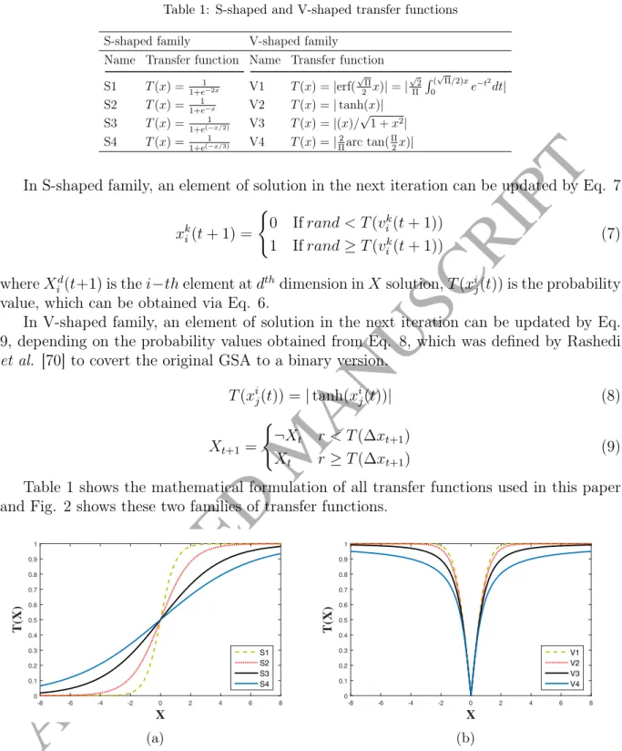
Table 1: S-shaped and V-shaped transfer functions

In S-shaped family, an element of solution in the next iteration can be updated by Eq. 7

xk_i(t+ 1) = ( 0 Ifrand < T(vk i(t+ 1)) 1 Ifrand_≥T(vk i(t+ 1)) (7) whereXd

i(t+1)is thei−thelement atdthdimension inXsolution,T(xij(t))is the probability

value, which can be obtained via Eq. 6.

In V-shaped family, an element of solution in the next iteration can be updated by Eq. 9, depending on the probability values obtained from Eq. 8, which was defined by Rashedi

et al. [70] to covert the original GSA to a binary version.

T(xi_j(t)) = |tanh(xi_j(t))| (8) Xt+1= ( ¬Xt r < T(∆xt+1) Xt r≥T(∆xt+1) (9) Table 1 shows the mathematical formulation of all transfer functions used in this paper and Fig. 2 shows these two families of transfer functions.

X -8 -6 -4 -2 0 2 4 6 8 T(X) 0 0.1 0.2 0.3 0.4 0.5 0.6 0.7 0.8 0.9 1 S1 S2 S3 S4 (a) X -8 -6 -4 -2 0 2 4 6 8 T(X) 0 0.1 0.2 0.3 0.4 0.5 0.6 0.7 0.8 0.9 1 V1 V2 V3 V4 (b)

Figure 2: Transfer functions families (a) S-shaped and (b) V-shaped.

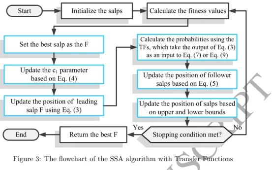
The flowchart of the the SSA algorithm with Transfer Functions is demonstrated in Fig. 3.

(11)

ACCEPTED MANUSCRIPT

Initialize the salps

Set the best salp as the F

Update the position of leading salp F using Eq. (3)

Calculate the probabilities using the TFs, which take the output of Eq. (3)

as an input to Eq. (7) or Eq. (9)

Update the position of follower salps based on Eq. (5) Update the position of salps based

on upper and lower bounds

Stopping condition met? Start

Yes No

Calculate the fitness values

Return the best F End

Update the c1parameter

based on Eq. (4)

Figure 3: The flowchart of the SSA algorithm with Transfer Functions

In the proposed BSSA, the leader’s position is updated by using a TF, while the followers’ positions are updated using Eq. 5. This equation calculates a solution between two given solutions, which is helpful when the variables are continuous. This equation is useless for binary problems since there are only two values for the variables. To address this issue, we employ a crossover operator to combine solutions as shown in Eq. 10.

xt_i+1=./(xi, xi−1) (10)

where./ is an operator that performs the crossover scheme on two binary solutions, and xi

is theith _{follower salp. An example of this process can be seen in Fig. 4.}

1 1 1 1 1 1 0 0 0 0 00 00 0 0 1 1 1 1 1 1 1 1 0 0 0 0 0 0 0 0 1 1 1 1 Randomly selected crossover point 1 0 1 0

Two initial salps

The final salps

Figure 4: The crossover process

It can be seen in Fig. 4 that the binary bits are exchanged between two solutions, which causes abrupt changes in both solution. This is the main mechanism of global search and exploration in the proposed BSSA algorithm. Note that the crossover operator aims to obtain an intermediate solution in a binary search space to mimic the concept of finding a

(12)

ACCEPTED MANUSCRIPT

solution between two solutions in Eq. 5. The crossover operator switches between two input vector with the same probability as given in Eq. 11.

xd = ( xd 1 rand≥0.5 xd 2 otherwise (11) wherexd _{is the value of the}_dth_{dimension in the resulted vector after applying the crossover}

operator onxi andxi−1.

The pseudocode of the proposed optimizer is presented in Algorithm 2

Algorithm 2 Pseudo-code of the SSA algorithm with Crossover operator Initialize the salp population xi(i= 1,2, . . . , n) consideringub andlb while (end condition is not satisfied)do

Calculate the fitness of each search agent (salp) SetF as the best search agent

Updatec1 by Eq. 4 for(each salp (xi)) do

if (i== 1)then

Update the position of the leading salp by Eq. 3

Calculate the probabilities using a TF which takes the output of Eq. 3 as its input (as in Eq. 7 (S-Shaped) or Eq. 9 (V-Shaped))

else

Update the position of the follower salp by performing a

Crossover operator betweenxi andxi−1 using Eq. 10.

Update the salps based on the upper and lower bounds of variables Return the best found solution F

5. Binary SSA for FS Problem

Two wrapper FS approaches that use SSA as a search algorithm and k-NN classifier as

an evaluator were proposed. To formulate FS as an optimization problem, two key points should be taken into consideration; how to represent a solution and how to evaluate it. In this work, a feature subset is represented as a binary vector with a length equals to the number of features in the dataset. If a feature is set to 1, this means that it has been selected, otherwise it has not. The goodness of a feature subset is measured depending on two criteria; the maximum classification accuracy (minimum error rate) and simultaneously the minimal number of selected features. These two contradict objectives are represented in one fitness function that is shown in Eq. 12:

↓F itness=αγR(D) +β|

R_|

|C| (12)

where γR(D) represents the classification error rate obtained by a specific classifier, |R| is

(13)

ACCEPTED MANUSCRIPT

the original dataset, and α _∈ [0,1], β = (1₋α) are two parameters corresponding to the

importance of classification quality and subset length as per recommendations in [41].

6. Experimental results and discussions

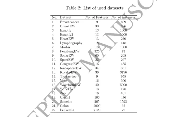
In this section, a comparative study is presented to carefully examine the exploratory and exploitative behavior of the proposed BSSA algorithms compared to several other well-established and novel metaheuristics. As case studies, 22 practical benchmark datasets are utilized. Table 2 describes these datasets in terms of number of features and number of instances. These datasets include several properties and cover various sizes and dimensions. For complete details about the origin and structure of these datasets, readers can refer to the sources available at UCI repository [71]. These problems can reveal the competency of the experienced optimizers in managing the exploration and exploitation trends and realizing more satisfactory results.

Table 2: List of used datasets

No. Dataset No. of Features No. of instances

1. Breastcancer 9 699 2. BreastEW 30 596 3. Exactly 13 1000 4. Exactly2 13 1000 5. HeartEW 13 270 6. Lymphography 18 148 7. M-of-n 13 1000 8. PenglungEW 325 73 9. SonarEW 60 208 10. SpectEW 22 267 11. CongressEW 16 435 12. IonosphereEW 34 351 13. KrvskpEW 36 3196 14. Tic-tac-toe 9 958 15. Vote 16 300 16. WaveformEW 40 5000 17. WineEW 13 178 18. Zoo 16 101 19. Clean1 166 476 20. Semeion 265 1593 21. Colon 2000 62 22. Leukemia 7129 72

The developed variants of BSSA are implemented to discover the superior reduct in terms of error rate using KNN classifier with a Euclidean distance metric (K= 5 [41]). To validate

the optimality of the results and substantiate the capabilities of algorithms, we use hold-out strategy where each dataset is randomly split into 80% for training and 20% for testing. To obtain statistically meaningful results, this split is repeated 30 independent times. Therefore, the statistical measurements are collected based on the overall capabilities and final results throughout 30 independent runs.The dimensions of the tackled problems are equal to number of features in the datasets.

All the tabulated evaluations and analyzed behaviors of the proposed BSSA are recorded and compared to other optimizers using a PC with Intel Core(TM) i5-5200U 2.2GHz CPU and 4.0GB RAM. All algorithms are tested using the MATLAB 2013 software. To have fair comparisons, all algorithms have been carefully implemented in the same programming language and by the same computing platform that can use the same global settings for all

(14)

ACCEPTED MANUSCRIPT

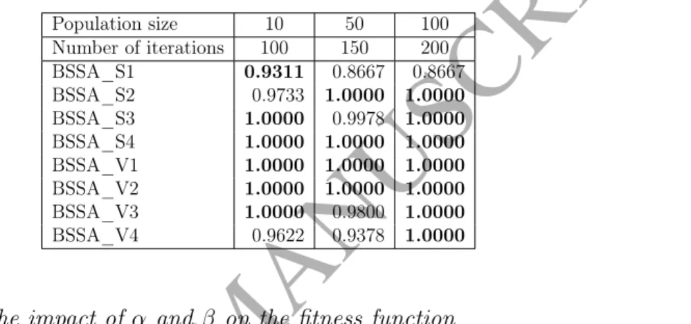
algorithms. That is, all algorithms are uniformly randomly initialized. Moreover, for all algorithms the population size is set to 10 search agents, and the number of iterations is set to 100. These values are selected after conducting an initial empirical study by experi-menting different values for the population size and number of iterations based on Leukemia dataset. This dataset was selected because it showed more sensitivity in comparison with other datasets. That is, significant changes in the performance of classifiers are noticed for slight changes in the parameter values [72]. As it can be seen in Table 3, a population size of 10 with 100 iterations managed to show very competitive results compared to larger population sizes and more iterations, which the latter require much more running time.

Table 3: Average accuracy results when using different combinations of population sizes and number of iterations based on Leukemia dataset.

Population size 10 50 100 Number of iterations 100 150 200 BSSA_S1 0.9311 0.8667 0.8667 BSSA_S2 0.9733 1.0000 1.0000 BSSA_S3 1.0000 0.9978 1.0000 BSSA_S4 1.0000 1.0000 1.0000 BSSA_V1 1.0000 1.0000 1.0000 BSSA_V2 1.0000 1.0000 1.0000 BSSA_V3 1.0000 0.9800 1.0000 BSSA_V4 0.9622 0.9378 1.0000

6.1. Assessment of the impact of α and β on the fitness function

The values of α and β in the fitness function reflect the weight of their corresponding

terms for the user. That is, α determines the weight of the classification accuracy, while β

corresponds to the weight of the features reduction rate. In majority of the previous works in literature, values of these parameters are set arbitrary. Traditionally,αis set to high value

(i.e. α≥0.90) andβ is set to a very small value (i.e. β ≤0.5). This experiment is conducted

to study the influence ofαandβ on the performance of the basic BSSA with different TFs.

The accuracy and the feature reduction rates are measured for different combinations of α

and β values. These experiments are conducted based on Leukemia dataset because this

dataset showed more sensitivity in comparison with other datasets. That is, significant changes in the performance of classifiers are noticed for slight changes in the parameter values [72]. The resulted accuracy rates are shown in Table 4, while the reduction rates are shown in Table 5. As it can be seen in the table, the accuracy rates are increased along with increasing the value of the α. On the other side, the impact of αand β on the feature

reduction rate is shown in Table 5. In general, there is a decrease in the reduction rate by decreasing the value ofβ.

In order to make fair comparisons with the obtained results in previous works, we will set α= 0.99 andβ= 0.01which are commonly used in the literature [41, 73].

6.2. Assessment of the proposed BSSA without crossover

In this subsection, the proposed BSSA-based algorithms are benchmarked on the 22 datasets to find the best version in dealing with FS problems. These binary versions utilize

(15)

ACCEPTED MANUSCRIPT

Table 4: Impact ofα andβ on the accuracy rates based on Leukemia dataset.

α 0.5 0.7 0.9 0.99

β 0.5 0.3 0.1 0.01

Transfer Functions AVE AVE AVE AVE BSSA_S1 0.8156 0.8578 0.8911 0.9311 BSSA_S2 0.9267 0.9578 0.9400 0.9733 BSSA_S3 0.9578 0.9778 1.0000 1.0000 BSSA_S4 0.8667 0.9333 0.9422 1.0000 BSSA_V1 0.8756 0.9422 0.9733 1.0000 BSSA_V2 0.8222 0.8867 0.9667 1.0000 BSSA_V3 0.9311 0.9689 0.9978 1.0000 BSSA_V4 0.9333 0.9578 0.9578 0.9622

Table 5: Impact ofαandβ on the feature reduction rate based on Leukemia dataset.

α 0.5 0.7 0.9 0.99

β 0.5 0.3 0.1 0.01

Transfer Functions AVE AVE AVE AVE BSSA_S1 0.5066 0.4495 0.4706 0.3852 BSSA_S2 0.5019 0.4671 0.4979 0.4166 BSSA_S3 0.4510 0.4572 0.4707 0.5102 BSSA_S4 0.4733 0.5014 0.5002 0.5088 BSSA_V1 0.5042 0.4934 0.4501 0.4796 BSSA_V2 0.5041 0.5055 0.4309 0.5086 BSSA_V3 0.5028 0.4879 0.5063 0.5081 BSSA_V4 0.5038 0.4917 0.4824 0.4455

different S-shaped and V-shaped transfer functions, which were reported in Table 1. The efficacy of the BSSA-based versions are evaluated in using the average classification accuracy measure, selection size, average fitness, running time, and convergence behaviors on different problems. The accuracy is studied based on the selected features of the evaluated cases. The standard deviation (STD) of the versions in realizing the datasets is reported as well for all comparisons. To compare the effectiveness of multiple transfer functions in BSSA optimizer and detect significant improvements, the average ranking of the Friedman test is utilized here.

Table 6 shows the average fitness (AVE) and STD results for eight versions of BSSA.Tables 7-9 similarly demonstrate the accuracy results, average number of features, and running time records accompanied by the STD and ranking results of all versions of the BSSA optimizer. From Table 6, it is seen that the BSSA_S1 can provide the best fitness re-sults on roughly 27% of the datasets. According to overall rankings, the best algorithm is the BSSA_V3, while the BSSA_S3, BSSA_S1, BSSA_S4, BSSA_V2, BSSA_S2, BSSA_V1, and BSSA_V4 are in the next stages.

Table 7 lists the results in terms of average accuracies. For the best and worst obtained accuracies we refer the reader to Table 25 in the appendix of tables. From Table 7, it can be seen that, in terms of classification accuracy, the BSSA with the first S-function outperforms all variants on around 27% of the datasets. The accuracy results of the binary version with V3 function are superior to those of other competitors according to overall rankings. According to the F-test results, those versions that utilize the S2, V1, and S4 transfer functions are in

(16)

ACCEPTED MANUSCRIPT

Table 6: Comparison between different versions of BSSA (without crossover) based on S-shaped and V-shaped transfer functions in terms of average fitness results

Benchmark Stat. Measure BSSA_S1 BSSA_S2 BSSA_S3 BSSA_S4 BSSA_V1 BSSA_V2 BSSA_V3 BSSA_V4 Breastcancer AVE 0.0293 0.0476 0.0308 0.0364 0.0393 0.0347 0.0377 0.0382 STD 0.0000 0.0005 0.0015 0.0011 0.0022 0.0011 0.0017 0.0009 BreastEW AVE 0.0583 0.0496 0.0466 0.0505 0.0528 0.0489 0.0487 0.0508 STD 0.0041 0.0035 0.0044 0.0034 0.0040 0.0050 0.0057 0.0037 Exactly AVE 0.0121 0.0162 0.0390 0.0211 0.0679 0.0740 0.0522 0.0771 STD 0.0135 0.0171 0.0333 0.0229 0.0665 0.0630 0.0560 0.0626 Exactly2 AVE 0.2804 0.2649 0.2431 0.2379 0.2402 0.2748 0.2336 0.2538 STD 0.0153 0.0089 0.0006 0.0056 0.0275 0.0125 0.0033 0.0233 HeartEW AVE 0.1572 0.1780 0.1939 0.1641 0.1826 0.1939 0.1734 0.1769 STD 0.0078 0.0116 0.0095 0.0105 0.0091 0.0103 0.0064 0.0100 Lymphography AVE 0.1326 0.1924 0.1551 0.1585 0.1393 0.1557 0.1824 0.1923 STD 0.0085 0.0109 0.0109 0.0128 0.0120 0.0150 0.0125 0.0146 M-of-n AVE 0.0093 0.0077 0.0186 0.0167 0.0304 0.0299 0.0277 0.0213 STD 0.0075 0.0050 0.0184 0.0119 0.0316 0.0319 0.0278 0.0209 PenglungEW AVE 0.1592 0.1041 0.1882 0.1773 0.0621 0.1497 0.1048 0.1184 STD 0.0117 0.0162 0.0141 0.0151 0.0093 0.0158 0.0115 0.0162 SonarEW AVE 0.1403 0.1310 0.1159 0.1298 0.1044 0.0679 0.1126 0.1566 STD 0.0097 0.0110 0.0136 0.0094 0.0104 0.0084 0.0117 0.0115 SpectEW AVE 0.1896 0.1456 0.1307 0.1551 0.1707 0.1570 0.1550 0.1790 STD 0.0077 0.0084 0.0090 0.0074 0.0052 0.0105 0.0090 0.0089 CongressEW AVE 0.0463 0.0395 0.0437 0.0335 0.0482 0.0249 0.0416 0.0302 STD 0.0050 0.0046 0.0050 0.0036 0.0039 0.0053 0.0042 0.0044 IonosphereEW AVE 0.1027 0.0807 0.0786 0.1139 0.0704 0.0728 0.0550 0.1006 STD 0.0054 0.0049 0.0067 0.0074 0.0074 0.0114 0.0053 0.0083 KrvskpEW AVE 0.0439 0.0348 0.0487 0.0450 0.0523 0.0518 0.0567 0.0500 STD 0.0048 0.0040 0.0038 0.0056 0.0081 0.0071 0.0067 0.0073 Tic-tac-toe AVE 0.2175 0.2120 0.1972 0.2247 0.1998 0.2154 0.2091 0.2114 STD 0.0000 0.0026 0.0041 0.0034 0.0063 0.0023 0.0029 0.0076 Vote AVE 0.0471 0.0541 0.0456 0.0337 0.0709 0.0597 0.0542 0.0493 STD 0.0058 0.0054 0.0035 0.0060 0.0052 0.0046 0.0036 0.0078 WaveformEW AVE 0.2671 0.2722 0.2703 0.2718 0.2773 0.2734 0.2838 0.2751 STD 0.0039 0.0057 0.0066 0.0052 0.0068 0.0081 0.0073 0.0071 WineEW AVE 0.0140 0.0412 0.0354 0.0256 0.0253 0.0279 0.0190 0.0288 STD 0.0049 0.0048 0.0044 0.0035 0.0069 0.0054 0.0087 0.0065 Zoo AVE 0.0704 0.0446 0.0047 0.0609 0.0486 0.0440 0.0427 0.0438 STD 0.0092 0.0005 0.0005 0.0064 0.0080 0.0006 0.0117 0.0009 Clean1 AVE 0.1592 0.1083 0.1100 0.1048 0.1327 0.1240 0.1080 0.1224 STD 0.0053 0.0049 0.0059 0.0059 0.0049 0.0073 0.0056 0.0081 Semeion AVE 0.0286 0.0299 0.0289 0.0369 0.0274 0.0304 0.0246 0.0259 STD 0.0014 0.0017 0.0012 0.0018 0.0016 0.0018 0.0018 0.0018 Colon AVE 0.1635 0.2630 0.2184 0.2894 0.2463 0.1670 0.2037 0.1570 STD 0.0058 0.0079 0.0152 0.0097 0.0242 0.0379 0.0248 0.0216 Leukemia AVE 0.0743 0.0322 0.0049 0.0049 0.0052 0.0049 0.0049 0.0429 STD 0.0118 0.0326 0.0000 0.0000 0.0006 0.0000 0.0000 0.0326 Ranking W|T|L 6|0|16 2|0|22 4|1|17 2|1|19 1|0|21 2|1|19 3|1|18 1|0|21

(17)

ACCEPTED MANUSCRIPT

Table 7: Comparison between different versions of BSSA (without crossover) based on S-shaped and V-shaped transfer functions in terms of average accuracy.

(18)

ACCEPTED MANUSCRIPT

the next places.

Table 8: Comparison between different versions of BSSA (without crossover) based on S-shaped and V-shaped transfer functions in terms of average number of features

Benchmark Stat. Measure BSSA_S1 BSSA_S2 BSSA_S3 BSSA_S4 BSSA_V1 BSSA_V2 BSSA_V3 BSSA_V4 Breastcancer AVE 6.0000 4.6333 4.8000 4.7333 5.0000 5.0667 5.2333 6.2333 STD 0.0000 0.4901 1.3493 0.9803 0.7428 0.9072 0.5040 0.4302 BreastEW AVE 19.8333 17.2000 16.0000 16.0667 14.5333 13.4333 13.8333 11.9333 STD 2.1669 2.5380 2.3342 2.6121 2.8129 3.4309 3.6111 3.2898 Exactly AVE 6.9667 7.0000 7.4000 7.2000 7.7000 7.8667 7.7000 7.7333 STD 0.6687 0.6433 0.7701 0.6644 1.0222 0.9371 1.0875 1.0483 Exactly2 AVE 9.2000 8.7333 2.0333 1.8000 1.9000 6.7667 1.8667 3.8667 STD 2.7342 0.7397 0.7649 1.2972 1.0619 2.4591 0.8996 3.3501 HeartEW AVE 6.9667 7.0000 8.0333 6.8333 7.9333 6.1000 6.4667 7.5000 STD 1.6291 1.4622 1.2726 1.2058 1.8182 1.5166 1.7564 1.4081 Lymphography AVE 13.1333 9.9000 10.2333 9.9667 9.1667 8.1333 8.1000 7.3333 STD 1.1366 1.3734 1.7357 1.5196 2.8416 3.0820 2.9167 2.1227 M-of-n AVE 6.9333 7.0333 7.2667 7.2000 7.7333 7.7333 7.3333 7.4333 STD 0.6915 0.5561 0.6397 0.7144 0.8683 1.0148 1.0283 0.9353 PenglungEW AVE 189.5000 195.4333 172.7333 167.7000 133.8667 111.0333 103.1333 109.1667 STD 25.5920 10.7405 9.1234 7.9791 40.3431 54.1113 55.9715 50.0221 SonarEW AVE 42.2667 39.8667 32.7333 30.7667 30.3667 30.6667 28.1667 27.6333 STD 3.0954 4.4313 2.6253 3.3081 3.2641 4.3417 4.2757 4.7524 SpectEW AVE 11.8000 12.0000 13.3000 10.6333 6.5000 11.1667 9.3333 10.2667 STD 2.1877 2.3342 2.0703 2.3413 3.6742 2.2907 2.5371 2.0331 CongressEW AVE 8.1333 7.0333 5.4333 5.9333 3.5333 7.3333 6.9000 4.4667 STD 1.2521 2.2047 1.4547 1.4840 2.2854 1.9885 1.6474 1.9954 IonosphereEW AVE 22.0333 18.9000 17.2667 14.3667 14.2667 13.7000 14.2667 12.5000 STD 3.5862 2.3831 3.0731 2.3706 2.7535 3.5926 3.3107 3.5307 KrvskpEW AVE 25.6667 22.2667 21.9000 21.6000 18.2000 18.4667 18.3000 18.2000 STD 2.1549 2.1324 2.3976 2.4719 4.4443 3.0141 3.4356 3.4978 Tic-tac-toe AVE 6.0000 6.0000 6.9000 5.2667 6.2333 6.3000 5.2667 6.0667 STD 0.0000 0.0000 0.3051 0.6915 0.8584 0.9154 0.5208 0.3651 Vote AVE 7.4667 5.9667 7.1333 5.7667 6.3667 5.7000 7.4667 5.3333 STD 1.2521 1.5862 2.1772 1.8696 2.0592 2.4233 2.7759 2.0734 WaveformEW AVE 30.4333 25.4000 23.3333 24.0667 22.0667 20.7000 22.4333 19.6333 STD 2.0457 2.8357 2.6305 2.7409 3.7318 4.1369 4.1163 3.2322 WineEW AVE 7.6333 6.3667 7.9667 6.8333 6.4333 6.3667 6.4000 5.6333 STD 0.8087 1.1592 2.0924 1.3917 1.6333 1.8286 1.5669 1.0662 Zoo AVE 8.1333 9.2667 7.5667 8.3333 8.4333 8.2667 8.2000 7.9667 STD 0.8996 0.7849 0.7739 1.0613 1.4308 0.9444 1.4239 1.3767 Clean1 AVE 115.5667 103.5667 93.2333 89.5000 76.7000 75.1000 75.5000 68.9667 STD 13.1193 7.4772 8.7678 5.6614 13.0758 14.8982 16.6604 16.7507 Semeion AVE 190.0333 166.2333 148.1333 140.8000 134.4000 129.4667 131.4000 132.2333 STD 23.1181 8.0288 7.3940 9.7994 7.7797 17.6728 7.3700 13.6904 Colon AVE 984.9000 1079.4333 1093.0000 1044.6667 502.8333 608.8000 710.2333 533.2333 STD 17.4224 105.4853 36.7283 31.5391 426.8525 418.4239 393.4634 381.6319 Leukemia AVE 4382.8000 4159.2670 3491.8670 3501.6670 3709.9670 3503.2670 3506.8670 3953.0670 STD 415.7237 346.0309 31.9145 23.3036 398.4409 25.7266 25.2870 632.9743 Ranking W|T|L 2|0|20 1|0|21 1|0|21 2|0|20 4|0|18 2|0|20 2|0|20 9|0|13 Overall Ranking F-Test 6.3182 5.6818 5.5909 4.3864 3.9545 3.7727 3.3636 2.9318

Inspecting the results in Table 8, it can be spotted that the proposed BSSA with V4 transfer function provides the lower number of features than others in around 41% of the datasets with the best ranking. Regarding the ranks, the BSSA with V-shaped transfer functions can provide better results than those with S-shaped functions.

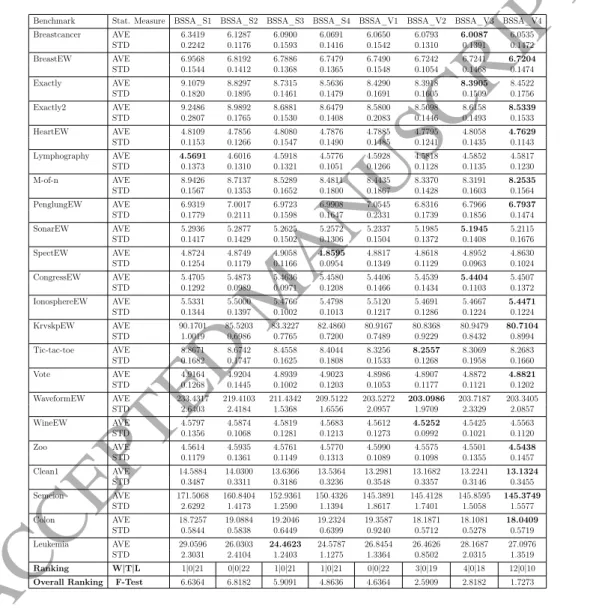
From Table 9, it is evident that the V4 can decrease the running time of the algorithm more than other choices. The transfer functions V2, V3, V1, S4, S3, S1, and S2 can be the next choices, respectively.

6.3. Assessment of the proposed BSSA with crossover

In this section we assess the performance of BSSA combined with crossover and compare its performance to the basic BSSA that has no crossover operator.

Table 10 reveals the average fitness results of the BSSA with S-shaped TFs and the proposed BSSA with crossover operator and S-shaped TFs. From this table, it is seen

(19)

ACCEPTED MANUSCRIPT

Table 9: Comparison between different versions of BSSA (without crossover) based on S-shaped and V-shaped transfer functions in terms of average running time

(20)

ACCEPTED MANUSCRIPT

that the BSSA_S3_CP and BSSA_S2_CP can significantly outperform the BSSA_S3 and BSSA_S3 on 73% of the datasets, respectively. The BSSA_S2_CP can disclose superior results compared to the BSSA_S2 in 54% of the datasets. The BSSA_S4_CP outperforms the BSSA_S4 on 68% problems. The reason is that the embedded crossover operator has enhanced the exploration capacity of BSSA_S3_CP and BSSA_S2_CP compared to those versions that utilize the standard average operator. Hence, in the case of premature con-vergence the BSSA-based methods with crossover theme have more chance to escape from them by more iteration and then, smoothly, switch from broad exploration to focused ex-ploitation around the food source. Based on the overall ranks at the end of Table 10, the BSSA_S3_CP have attained the best rank among other competitors in terms of the average fitness values.

Table 10: Comparison between the BSSA with S-shaped functions (without crossover) and the proposed BSSA combined with CP in terms of average fitness results.

Benchmark Stat. Measure BSSA_S1 BSSA_S1_CP BSSA_S2 BSSA_S2_CP BSSA_S3 BSSA_S3_CP BSSA_S4 BSSA_S4_CP Breastcancer AVE 0.0293 0.0447 0.0476 0.0312 0.0308 0.0273 0.0364 0.0227 STD 0.0000 0.0019 0.0005 0.0032 0.0015 0.0006 0.0011 0.0005 BreastEW AVE 0.0583 0.0448 0.0496 0.0551 0.0466 0.0566 0.0505 0.0442 STD 0.0041 0.0035 0.0035 0.0056 0.0044 0.0033 0.0034 0.0030 Exactly AVE 0.0121 0.0146 0.0162 0.0088 0.0390 0.0251 0.0211 0.0231 STD 0.0135 0.0127 0.0171 0.0047 0.0333 0.0254 0.0229 0.0211 Exactly2 AVE 0.2804 0.2561 0.2649 0.2512 0.2431 0.2415 0.2379 0.2818 STD 0.0153 0.0081 0.0089 0.0107 0.0006 0.0197 0.0056 0.0073 HeartEW AVE 0.1572 0.1711 0.1780 0.1691 0.1939 0.1426 0.1641 0.1604 STD 0.0078 0.0053 0.0116 0.0075 0.0095 0.0074 0.0105 0.0077 Lymphography AVE 0.1326 0.1674 0.1924 0.1630 0.1551 0.1146 0.1585 0.1332 STD 0.0085 0.0092 0.0109 0.0118 0.0109 0.0108 0.0128 0.0085 M-of-n AVE 0.0093 0.0076 0.0077 0.0064 0.0186 0.0136 0.0167 0.0115 STD 0.0075 0.0068 0.0050 0.0043 0.0184 0.0136 0.0119 0.0079 PenglungEW AVE 0.1592 0.0853 0.1041 0.2147 0.1882 0.1266 0.1773 0.0816 STD 0.0117 0.0084 0.0162 0.0098 0.0141 0.0134 0.0151 0.0091 SonarEW AVE 0.1403 0.0776 0.1310 0.1100 0.1159 0.0678 0.1298 0.1131 STD 0.0097 0.0076 0.0110 0.0105 0.0136 0.0095 0.0094 0.0098 SpectEW AVE 0.1896 0.1479 0.1456 0.1632 0.1307 0.1673 0.1551 0.1678 STD 0.0077 0.0050 0.0084 0.0067 0.0090 0.0044 0.0074 0.0082 CongressEW AVE 0.0463 0.0375 0.0395 0.0345 0.0437 0.0404 0.0335 0.0386 STD 0.0050 0.0056 0.0046 0.0033 0.0050 0.0037 0.0036 0.0052 IonosphereEW AVE 0.1027 0.1413 0.0807 0.0762 0.0786 0.0857 0.1139 0.1000 STD 0.0054 0.0059 0.0049 0.0048 0.0067 0.0080 0.0074 0.0059 KrvskpEW AVE 0.0439 0.0411 0.0348 0.0397 0.0487 0.0410 0.0450 0.0446 STD 0.0048 0.0037 0.0040 0.0047 0.0038 0.0058 0.0056 0.0068 Tic-tac-toe AVE 0.2175 0.2135 0.2120 0.2222 0.1972 0.1844 0.2247 0.2098 STD 0.0000 0.0069 0.0026 0.0028 0.0041 0.0000 0.0034 0.0038 Vote AVE 0.0471 0.0420 0.0541 0.0523 0.0456 0.0514 0.0337 0.0549 STD 0.0058 0.0093 0.0054 0.0032 0.0035 0.0057 0.0060 0.0042 WaveformEW AVE 0.2671 0.2709 0.2722 0.2658 0.2703 0.2695 0.2718 0.2711 STD 0.0039 0.0047 0.0057 0.0061 0.0066 0.0071 0.0052 0.0072 WineEW AVE 0.0140 0.0077 0.0412 0.0279 0.0354 0.0115 0.0256 0.0350 STD 0.0049 0.0035 0.0048 0.0021 0.0044 0.0057 0.0035 0.0043 Zoo AVE 0.0704 0.1015 0.0446 0.0438 0.0047 0.0042 0.0609 0.0401 STD 0.0092 0.0155 0.0005 0.0005 0.0005 0.0004 0.0064 0.0064 Clean1 AVE 0.1592 0.1168 0.1083 0.1051 0.1100 0.1248 0.1048 0.1079 STD 0.0053 0.0068 0.0049 0.0048 0.0059 0.0041 0.0059 0.0067 Semeion AVE 0.0286 0.0322 0.0299 0.0338 0.0289 0.0255 0.0369 0.0308 STD 0.0014 0.0017 0.0017 0.0016 0.0012 0.0014 0.0018 0.0015 Colon AVE 0.1635 0.2464 0.2630 0.1390 0.2184 0.3163 0.2894 0.1255 STD 0.0058 0.0156 0.0079 0.0119 0.0152 0.0185 0.0097 0.0137 Leukemia AVE 0.0743 0.0123 0.0322 0.0051 0.0049 0.0166 0.0049 0.0765 STD 0.0118 0.0199 0.0326 0.0003 0.0000 0.0247 0.0000 0.0165 Ranking W|T|L 9|0|13 13|0|9 6|0|16 16|0|6 7|0|15 15|0|7 8|0|14 14|0|8

Overall Ranking F-Test 4.8636 4.2727 5.2273 3.8182 4.7727 3.6818 5.0909 4.2727

In Table 11 we list the fitness results of the proposed BSSA methods with V-shaped TFs.According to this table, it is observed that the BSSA_V2_CP can obtain significantly

(21)

ACCEPTED MANUSCRIPT

better fitness measures than the BSSA_V2 on 59% of the datasets. The crossover operator has also improved the fitness values of BSSA_V4 algorithm on 12 cases. The reason is that the crossover operator improves the exploratory characteristic of the BSSA_V2 and BSSA_V4 variants. As such, it can jump out of sub-optimal solutions more efficiently, whereas the other competitors are still disposed to stagnation to local solutions. Based on the overall ranks, the BSSA with V2 and CP has demonstrated a better efficacy than other techniques.

Table 11: Comparison between the BSSA with V-shaped functions and the proposed BSSA with CP regarding the average fitness results.

Benchmark Stat. Measure BSSA_V1 BSSA_V1_CP BSSA_V2 BSSA_V2_CP BSSA_V3 BSSA_V3_CP BSSA_V4 BSSA_V4_CP Breastcancer AVE 0.0393 0.0331 0.0347 0.0278 0.0377 0.0324 0.0382 0.0371 STD 0.0022 0.0007 0.0011 0.0016 0.0017 0.0005 0.0009 0.0029 BreastEW AVE 0.0528 0.0435 0.0489 0.0385 0.0487 0.0640 0.0508 0.0445 STD 0.0040 0.0042 0.0050 0.0041 0.0057 0.0049 0.0037 0.0039 Exactly AVE 0.0679 0.0390 0.0740 0.0467 0.0522 0.0413 0.0771 0.0294 STD 0.0665 0.0446 0.0630 0.0527 0.0560 0.0370 0.0626 0.0286 Exactly2 AVE 0.2402 0.2639 0.2748 0.2448 0.2336 0.2838 0.2538 0.2727 STD 0.0275 0.0127 0.0125 0.0005 0.0033 0.0089 0.0233 0.0120 HeartEW AVE 0.1826 0.1767 0.1939 0.1714 0.1734 0.1779 0.1769 0.1820 STD 0.0091 0.0104 0.0103 0.0080 0.0064 0.0099 0.0100 0.0101 Lymphography AVE 0.1393 0.1581 0.1557 0.1382 0.1824 0.1958 0.1923 0.1520 STD 0.0120 0.0142 0.0150 0.0149 0.0125 0.0109 0.0146 0.0169 M-of-n AVE 0.0304 0.0163 0.0299 0.0192 0.0277 0.0318 0.0213 0.0243 STD 0.0316 0.0146 0.0319 0.0236 0.0278 0.0370 0.0209 0.0235 PenglungEW AVE 0.0621 0.1752 0.1497 0.0844 0.1048 0.1183 0.1184 0.1237 STD 0.0093 0.0185 0.0158 0.0008 0.0115 0.0174 0.0162 0.0135 SonarEW AVE 0.1044 0.1139 0.0679 0.1014 0.1126 0.1021 0.1566 0.1062 STD 0.0104 0.0125 0.0084 0.0075 0.0117 0.0105 0.0115 0.0110 SpectEW AVE 0.1707 0.1948 0.1570 0.1771 0.1550 0.1337 0.1790 0.1693 STD 0.0052 0.0131 0.0105 0.0096 0.0090 0.0061 0.0089 0.0116 CongressEW AVE 0.0482 0.0317 0.0249 0.0438 0.0416 0.0456 0.0302 0.0306 STD 0.0039 0.0036 0.0053 0.0061 0.0042 0.0058 0.0044 0.0095 IonosphereEW AVE 0.0704 0.0924 0.0728 0.1089 0.0550 0.0886 0.1006 0.0949 STD 0.0074 0.0066 0.0114 0.0100 0.0053 0.0089 0.0083 0.0076 KrvskpEW AVE 0.0523 0.0508 0.0518 0.0604 0.0567 0.0512 0.0500 0.0521 STD 0.0081 0.0095 0.0071 0.0069 0.0067 0.0079 0.0073 0.0069 Tic-tac-toe AVE 0.1998 0.2170 0.2154 0.2162 0.2091 0.2022 0.2114 0.2245 STD 0.0063 0.0016 0.0023 0.0038 0.0029 0.0085 0.0076 0.0053 Vote AVE 0.0709 0.0465 0.0597 0.0440 0.0542 0.0336 0.0493 0.0368 STD 0.0052 0.0053 0.0046 0.0063 0.0036 0.0038 0.0078 0.0053 WaveformEW AVE 0.2773 0.2707 0.2734 0.2767 0.2838 0.2702 0.2751 0.2806 STD 0.0068 0.0059 0.0081 0.0079 0.0073 0.0057 0.0071 0.0083 WineEW AVE 0.0253 0.0437 0.0279 0.0228 0.0190 0.0249 0.0288 0.0267 STD 0.0069 0.0052 0.0054 0.0052 0.0087 0.0110 0.0065 0.0056 Zoo AVE 0.0486 0.0299 0.0440 0.0605 0.0427 0.0446 0.0438 0.0040 STD 0.0080 0.0137 0.0006 0.0059 0.0117 0.0048 0.0009 0.0006 Clean1 AVE 0.1327 0.1149 0.1240 0.1082 0.1080 0.1020 0.1224 0.1242 STD 0.0049 0.0085 0.0073 0.0077 0.0056 0.0082 0.0081 0.0062 Semeion AVE 0.0274 0.0293 0.0304 0.0295 0.0246 0.0336 0.0259 0.0238 STD 0.0016 0.0016 0.0018 0.0021 0.0018 0.0015 0.0018 0.0018 Colon AVE 0.2463 0.2535 0.1670 0.1875 0.2037 0.1433 0.1570 0.3530 STD 0.0242 0.0503 0.0379 0.0335 0.0248 0.0286 0.0216 0.1000 Leukemia AVE 0.0052 0.0049 0.0049 0.0051 0.0049 0.0049 0.0429 0.0365 STD 0.0006 0.0000 0.0000 0.0004 0.0000 0.0000 0.0326 0.0328 Ranking W|T|L 10|0|12 12|0|10 10|0|12 12|0|10 10|1|11 10|1|11 10|0|12 12|0|10

Overall Ranking F-Test 5 4.409 4.9091 3.8182 4.0909 4.1364 5.0455 4.5909

Table 12 reveals the average results of proposed methods with S-shaped TFs. The supe-rior accuracies of the BSSA with crossover operator can be detected on majority of datasets. The reason is that it can make a more stable balance between the diversification and in-tensification leanings due to its effective crossover operator between the candidate salps. Based on the ranking orders, the BSSA with S2 function and crossover strategy is the best algorithm among other optimizers. It is capable of providing higher accuracies than other

(22)

ACCEPTED MANUSCRIPT

optimizers on 68% of the datasets when showing acceptable STD values.

Table 12: Comparison between the BSSA with S-Shaped TFs approaches and the proposed method (with CP) based on the average accuracy.

Benchmark Stat. Measure BSSA_S1 BSSA_S1_CP BSSA_S2 BSSA_S2_CP BSSA_S3 BSSA_S3_CP BSSA_S4 BSSA_S4_CP Breastcancer AVE 0.9771 0.9608 0.9571 0.9724 0.9743 0.9768 0.9686 0.9829 STD 0.0000 0.0017 0.0000 0.0027 0.0000 0.0010 0.0000 0.0000 BreastEW AVE 0.9478 0.9616 0.9557 0.9505 0.9584 0.9484 0.9544 0.9603 STD 0.0041 0.0036 0.0036 0.0056 0.0046 0.0035 0.0033 0.0029 Exactly AVE 0.9932 0.9905 0.9891 0.9963 0.9663 0.9803 0.9843 0.9823 STD 0.0132 0.0125 0.0169 0.0046 0.0332 0.0253 0.0227 0.0209 Exactly2 AVE 0.7239 0.7480 0.7392 0.7509 0.7560 0.7582 0.7611 0.7224 STD 0.0134 0.0078 0.0087 0.0092 0.0000 0.0183 0.0047 0.0078 HeartEW AVE 0.8467 0.8336 0.8257 0.8338 0.8104 0.8605 0.8395 0.8432 STD 0.0071 0.0050 0.0113 0.0072 0.0096 0.0070 0.0107 0.0073 Lymphography AVE 0.8734 0.8369 0.8113 0.8410 0.8491 0.8900 0.8455 0.8707 STD 0.0090 0.0093 0.0109 0.0121 0.0113 0.0110 0.0131 0.0085 M-of-n AVE 0.9960 0.9976 0.9977 0.9987 0.9869 0.9918 0.9887 0.9941 STD 0.0072 0.0066 0.0047 0.0041 0.0181 0.0133 0.0116 0.0076 PenglungEW AVE 0.8450 0.9198 0.9009 0.7883 0.8153 0.8775 0.8261 0.9225 STD 0.0122 0.0086 0.0164 0.0102 0.0143 0.0137 0.0154 0.0093 SonarEW AVE 0.8654 0.9285 0.8744 0.8949 0.8885 0.9372 0.8740 0.8910 STD 0.0098 0.0079 0.0113 0.0107 0.0137 0.0097 0.0096 0.0099 SpectEW AVE 0.8139 0.8565 0.8585 0.8418 0.8741 0.8361 0.8483 0.8356 STD 0.0078 0.0051 0.0084 0.0072 0.0091 0.0054 0.0072 0.0082 CongressEW AVE 0.9584 0.9668 0.9645 0.9697 0.9593 0.9628 0.9699 0.9645 STD 0.0050 0.0053 0.0047 0.0037 0.0051 0.0035 0.0035 0.0048 IonosphereEW AVE 0.9028 0.8634 0.9241 0.9286 0.9258 0.9182 0.8892 0.9034 STD 0.0055 0.0059 0.0048 0.0051 0.0068 0.0081 0.0076 0.0058 KrvskpEW AVE 0.9629 0.9657 0.9711 0.9661 0.9570 0.9644 0.9606 0.9607 STD 0.0048 0.0036 0.0037 0.0046 0.0036 0.0059 0.0055 0.0067 Tic-tac-toe AVE 0.7871 0.7902 0.7926 0.7822 0.8086 0.8205 0.7789 0.7939 STD 0.0000 0.0065 0.0026 0.0031 0.0045 0.0000 0.0029 0.0033 Vote AVE 0.9571 0.9629 0.9491 0.9529 0.9584 0.9511 0.9696 0.9489 STD 0.0057 0.0092 0.0057 0.0035 0.0042 0.0059 0.0060 0.0040 WaveformEW AVE 0.7379 0.7337 0.7315 0.7381 0.7328 0.7335 0.7316 0.7321 STD 0.0039 0.0045 0.0056 0.0060 0.0067 0.0069 0.0052 0.0072 WineEW AVE 0.9918 0.9985 0.9633 0.9772 0.9704 0.9933 0.9794 0.9708 STD 0.0051 0.0039 0.0051 0.0021 0.0055 0.0056 0.0043 0.0056 Zoo AVE 0.9340 0.9026 0.9608 0.9608 1.0000 1.0000 0.9438 0.9634 STD 0.0096 0.0159 0.0000 0.0000 0.0000 0.0000 0.0068 0.0068 Clean1 AVE 0.8462 0.8894 0.8969 0.8999 0.8945 0.8796 0.8996 0.8962 STD 0.0057 0.0067 0.0050 0.0049 0.0060 0.0042 0.0060 0.0068 Semeion AVE 0.9783 0.9749 0.9762 0.9721 0.9764 0.9799 0.9681 0.9744 STD 0.0014 0.0018 0.0018 0.0018 0.0012 0.0015 0.0018 0.0015 Colon AVE 0.8398 0.7570 0.7398 0.8656 0.7849 0.6860 0.7129 0.8785 STD 0.0059 0.0164 0.0082 0.0122 0.0155 0.0188 0.0098 0.0139 Leukemia AVE 0.9311 0.9933 0.9733 1.0000 1.0000 0.9889 1.0000 0.9289 STD 0.0122 0.0203 0.0332 0.0000 0.0000 0.0253 0.0000 0.0169 Ranking W|T|L 9|0|13 13|0|9 6|1|15 15|1|6 7|1|14 14|1|7 8|0|14 14|0|8 Overall Ranking F-Test 4.7955 4.0909 5.0455 3.75 4.7955 3.9091 5.1818 4.4318

Table 13 tabulates the average accuracy results of the proposed methods with V-shaped TFs. For the best and worst obtained accuracies we refer the reader to Table 25 in the appendix of tables. From Table 13, it is observed that the accuracies have been increased in those cases that utilize both crossover operator and V-shaped transfer formula. For instance, the BSSA_V1_CP, BSSA_V2_CP and BSSA_V4_CP show higher classification rates than those of their competitors on Breastcancer, BreastEW, and Exactly datasets. The enriched searching patterns of algorithms with crossover scheme can be detected from their improved results on different datasets compared to other binary versions. By comparing the BSSA_V3 with BSSA_V3_CP, it is seen that each method has outperformed other one on 11 datasets and both methods have achieved to a similar rank. Regarding the overall ranks, the BSSA_V2_CP can be selected as the best version.

The average number of features found by BSSA-based techniques with S-shaped TFs are revealed in Table 14. As it can be seen, both BSSA_S4 and BSSA_S4_CP are similarly

(23)

ACCEPTED MANUSCRIPT

Table 13: Comparison between the BSSA with V-Shaped TFs approaches and the related version with CP based on average accuracy.

Benchmark Stat. Measure BSSA_V1 BSSA_V1_CP BSSA_V2 BSSA_V2_CP BSSA_V3 BSSA_V3_CP BSSA_V4 BSSA_V4_CP Breastcancer AVE 0.9659 0.9713 0.9707 0.9767 0.9678 0.9735 0.9684 0.9695 STD 0.0025 0.0005 0.0018 0.0017 0.0018 0.0013 0.0007 0.0026 BreastEW AVE 0.9516 0.9608 0.9551 0.9661 0.9554 0.9400 0.9528 0.9601 STD 0.0042 0.0040 0.0046 0.0044 0.0053 0.0049 0.0038 0.0042 Exactly AVE 0.9374 0.9663 0.9313 0.9586 0.9533 0.9640 0.9281 0.9759 STD 0.0665 0.0445 0.0629 0.0526 0.0558 0.0369 0.0625 0.0284 Exactly2 AVE 0.7589 0.7354 0.7277 0.7540 0.7655 0.7203 0.7467 0.7302 STD 0.0270 0.0106 0.0119 0.0000 0.0029 0.0089 0.0212 0.0129 HeartEW AVE 0.8217 0.8262 0.8089 0.8316 0.8299 0.8252 0.8272 0.8215 STD 0.0101 0.0108 0.0104 0.0080 0.0071 0.0102 0.0109 0.0104 Lymphography AVE 0.8644 0.8459 0.8473 0.8650 0.8203 0.8068 0.8099 0.8509 STD 0.0125 0.0153 0.0155 0.0151 0.0129 0.0113 0.0154 0.0172 M-of-n AVE 0.9753 0.9891 0.9758 0.9863 0.9777 0.9735 0.9843 0.9813 STD 0.0315 0.0141 0.0315 0.0233 0.0274 0.0368 0.0205 0.0231 PenglungEW AVE 0.9414 0.8270 0.8523 0.9189 0.8973 0.8847 0.8838 0.8793 STD 0.0102 0.0182 0.0154 0.0000 0.0110 0.0173 0.0161 0.0137 SonarEW AVE 0.8997 0.8894 0.9365 0.9022 0.8910 0.9016 0.8465 0.8974 STD 0.0106 0.0126 0.0086 0.0076 0.0119 0.0106 0.0117 0.0114 SpectEW AVE 0.8306 0.8072 0.8465 0.8236 0.8478 0.8699 0.8239 0.8331 STD 0.0056 0.0132 0.0109 0.0101 0.0091 0.0064 0.0093 0.0117 CongressEW AVE 0.9535 0.9708 0.9795 0.9587 0.9624 0.9564 0.9723 0.9713 STD 0.0036 0.0039 0.0056 0.0058 0.0042 0.0055 0.0044 0.0089 IonosphereEW AVE 0.9331 0.9106 0.9305 0.8938 0.9487 0.9136 0.9021 0.9078 STD 0.0074 0.0067 0.0110 0.0097 0.0053 0.0086 0.0081 0.0069 KrvskpEW AVE 0.9523 0.9540 0.9529 0.9447 0.9479 0.9536 0.9546 0.9525 STD 0.0086 0.0097 0.0072 0.0071 0.0068 0.0081 0.0074 0.0072 Tic-tac-toe AVE 0.8052 0.7868 0.7895 0.7875 0.7947 0.8025 0.7933 0.7800 STD 0.0074 0.0011 0.0020 0.0034 0.0027 0.0086 0.0076 0.0054 Vote AVE 0.9324 0.9558 0.9433 0.9589 0.9500 0.9696 0.9536 0.9662 STD 0.0057 0.0054 0.0045 0.0063 0.0042 0.0042 0.0075 0.0055 WaveformEW AVE 0.7255 0.7321 0.7291 0.7256 0.7190 0.7323 0.7271 0.7219 STD 0.0068 0.0058 0.0077 0.0077 0.0072 0.0058 0.0071 0.0082 WineEW AVE 0.9794 0.9610 0.9768 0.9820 0.9858 0.9794 0.9753 0.9779 STD 0.0073 0.0057 0.0051 0.0056 0.0093 0.0111 0.0069 0.0055 Zoo AVE 0.9562 0.9739 0.9608 0.9431 0.9621 0.9595 0.9608 1.0000 STD 0.0084 0.0139 0.0000 0.0060 0.0114 0.0050 0.0000 0.0000 Clean1 AVE 0.8706 0.8882 0.8793 0.8955 0.8955 0.9020 0.8805 0.8793 STD 0.0050 0.0082 0.0071 0.0076 0.0055 0.0084 0.0079 0.0061 Semeion AVE 0.9774 0.9754 0.9742 0.9751 0.9801 0.9710 0.9789 0.9808 STD 0.0017 0.0016 0.0019 0.0021 0.0019 0.0013 0.0017 0.0018 Colon AVE 0.7538 0.7473 0.8344 0.8140 0.7978 0.8581 0.8441 0.6462 STD 0.0232 0.0495 0.0367 0.0325 0.0239 0.0276 0.0209 0.0993 Leukemia AVE 1.0000 1.0000 1.0000 1.0000 1.0000 1.0000 0.9622 0.9689 STD 0.0000 0.0000 0.0000 0.0000 0.0000 0.0000 0.0336 0.0338 Ranking W|T|L 10|1|11 11|1|10 9|1|12 12|1|9 11|1|10 10|1|11 10|0|12 12|0|10 Overall Ranking F-Test 4.9318 4.4545 4.9091 3.8409 4.1591 4.1591 4.9318 4.6136

(24)

ACCEPTED MANUSCRIPT

the best choices in terms of selected features.

Table 14: Comparison between the BSSA based S-Shaped transfer functions approaches and the proposed method (with CP) based on average number of features.

Benchmark Stat. Measure BSSA_S1 BSSA_S1_CP BSSA_S2 BSSA_S2_CP BSSA_S3 BSSA_S3_CP BSSA_S4 BSSA_S4_CP

Breastcancer AVE 6.0000 5.2333 4.6333 3.4333 4.8000 3.8667 4.7333 5.2000 STD 0.0000 0.4302 0.4901 0.5040 1.3493 0.3457 0.9803 0.4068 BreastEW AVE 19.8333 20.5000 17.2000 18.3667 16.0000 16.7000 16.0667 14.8333 STD 2.1669 1.7568 2.5380 2.8099 2.3342 2.3364 2.6121 1.8770 Exactly AVE 6.9667 6.8000 7.0000 6.7000 7.4000 7.2000 7.2000 7.3333 STD 0.6687 0.5509 0.6433 0.4661 0.7701 0.6644 0.6644 0.6065 Exactly2 AVE 9.2000 8.6333 8.7333 6.0333 2.0333 2.7333 1.8000 9.1333 STD 2.7342 1.6291 0.7397 2.6193 0.7649 2.3916 1.2972 1.0743 HeartEW AVE 6.9667 8.3000 7.0000 6.0000 8.0333 5.8000 6.8333 6.6667 STD 1.6291 0.5350 1.4622 1.3646 1.2726 1.4239 1.2058 1.3218 Lymphography AVE 13.1333 10.8000 9.9000 10.0000 10.2333 10.2667 9.9667 9.4667 STD 1.1366 0.9613 1.3734 1.2318 1.7357 1.9286 1.5196 1.8333 M-of-n AVE 6.9333 6.8333 7.0333 6.7333 7.2667 7.1000 7.2000 7.3000 STD 0.6915 0.5307 0.5561 0.6397 0.6397 0.6618 0.7144 0.6513 PenglungEW AVE 189.5000 193.5000 195.4333 166.8333 172.7333 171.6000 167.7000 159.9000 STD 25.5920 19.3333 10.7405 15.1887 9.1234 9.9329 7.9791 5.9385 SonarEW AVE 42.2667 41.1333 39.8667 35.6667 32.7333 33.3667 30.7667 31.1000 STD 3.0954 3.6173 4.4313 2.9866 2.6253 2.8585 3.3081 2.6044 SpectEW AVE 11.8000 12.7667 12.0000 14.4667 13.3000 10.9333 10.6333 11.0333 STD 2.1877 1.6121 2.3342 2.4457 2.0703 3.5809 2.3413 1.6709 CongressEW AVE 8.1333 7.4000 7.0333 7.2000 5.4333 5.7333 5.9333 5.5333 STD 1.2521 1.6103 2.2047 1.8644 1.4547 1.3629 1.4840 1.6965 IonosphereEW AVE 22.0333 20.8333 18.9000 18.8333 17.2667 15.8667 14.3667 14.9333 STD 3.5862 2.4925 2.3831 2.5875 3.0731 2.5829 2.3706 2.4486 KrvskpEW AVE 25.6667 25.7333 22.2667 21.9667 21.9000 20.4667 21.6000 20.5667 STD 2.1549 2.1324 2.1324 2.3706 2.3976 2.5560 2.4719 2.3735 Tic-tac-toe AVE 6.0000 5.2333 6.0000 5.9000 6.9000 6.0000 5.2667 5.2000 STD 0.0000 0.5040 0.0000 0.3051 0.3051 0.0000 0.6915 0.4842 Vote AVE 7.4667 8.4667 5.9667 9.0333 7.1333 4.8333 5.7667 6.9000 STD 1.2521 1.4077 1.5862 1.5421 2.1772 1.4875 1.8696 1.8634 WaveformEW AVE 30.4333 28.7667 25.4000 25.8333 23.3333 22.9000 24.0667 23.6000 STD 2.0457 2.6997 2.8357 2.6663 2.6305 3.3255 2.7409 3.0468 WineEW AVE 7.6333 8.1333 6.3667 6.8333 7.9667 6.3333 6.8333 7.8667 STD 0.8087 1.6554 1.1592 1.2617 2.0924 0.9589 1.3917 2.1772 Zoo AVE 8.1333 8.2000 9.2667 7.9333 7.5667 6.7000 8.3333 6.1667 STD 0.8996 1.1567 0.7849 0.7397 0.7739 0.7022 1.0613 0.8743 Clean1 AVE 115.5667 120.0667 103.5667 99.7333 93.2333 92.1667 89.5000 86.4000 STD 13.1193 8.4115 7.4772 6.6381 8.7678 6.2427 5.6614 7.2853 Semeion AVE 190.0333 196.9000 166.2333 165.9000 148.1333 147.5000 140.8000 143.2000 STD 23.1181 10.3968 8.0288 14.5705 7.3940 8.7168 9.7994 7.2844 Colon AVE 984.9000 1160.8333 1079.4333 1180.7000 1093.0000 1097.4333 1044.6667 1049.2333 STD 17.4224 152.8493 105.4853 85.4312 36.7283 44.7165 31.5391 22.2272 Leukemia AVE 4382.8000 4063.0333 4159.2670 3642.5000 3491.8670 3959.9333 3501.6670 4326.3667 STD 415.7237 482.5962 346.0309 235.9664 31.9145 530.6809 23.3036 515.6235 Ranking W|T|L 11|0|11 11|0|11 8|0|14 14|0|8 7|0|15 15|0|7 12|0|10 10|0|12 Overall Ranking F-Test 6.1364 6.2727 5.1818 4.5227 4.5455 3.2500 3.0455 3.0455

Inspecting the average number of features attained by BSSA-based algorithms with V-shaped TFs in Table 15, we can notice that the BSSA_V2_CP version has obtained the best place among other versions. The reason is that the crossover operator has enhanced the searching competences of the BSSA_V2_CP on majority of tasks.

Average running time of BSSA-based optimizers with S-shaped TFs are shown in Table 16. Inspecting the results in in this table, the BSSA_S3_CP is the best approach among others. On the other hand, Table 17 compares the the running time of the BSSA-based algorithms with V-shaped TFs.It can be noticed that the BSSA_V4_CP algorithm has the lowest average running time. From the running time results in Tables 16 and 17, it is evident that BSSA-based versions that utilize the crossover strategy beside the S-shaped and V-shaped TFs can perform the exploration and exploitation phases better and quicker than other binary versions that still employ the average operator of the basic SSA.

(25)

ACCEPTED MANUSCRIPT

Table 15: Comparison between the BSSA based V-Shaped transfer functions approaches and the proposed method (with CP) based on average number of features.

Benchmark Stat. Measure BSSA_V1 BSSA_V1_CP BSSA_V2 BSSA_V2_CP BSSA_V3 BSSA_V3_CP BSSA_V4 BSSA_V4_CP

Breastcancer AVE 5.0000 4.2667 5.0667 4.2000 5.2333 5.5667 6.2333 6.2667 STD 0.7428 0.4498 0.9072 0.5509 0.5040 0.7739 0.4302 0.4498 BreastEW AVE 14.5333 14.0000 13.4333 14.8333 13.8333 13.6667 11.9333 15.1667 STD 2.8129 2.5052 3.4309 3.1082 3.6111 2.9165 3.2898 2.4925 Exactly AVE 7.7000 7.3333 7.8667 7.4000 7.7000 7.4000 7.7333 7.3000 STD 1.0222 0.8023 0.9371 0.9685 1.0875 0.7701 1.0483 0.7497 Exactly2 AVE 1.9000 2.4667 6.7667 1.6000 1.8667 9.0333 3.8667 7.2667 STD 1.0619 2.9212 2.4591 0.6215 0.8996 1.0334 3.3501 2.1961 HeartEW AVE 7.9333 6.0000 6.1000 6.1000 6.4667 6.2333 7.5000 6.8667 STD 1.8182 1.2318 1.5166 0.9948 1.7564 0.8584 1.4081 1.0743 Lymphography AVE 9.1667 10.0333 8.1333 8.2667 8.1000 8.0333 7.3333 7.9000 STD 2.8416 2.4980 3.0820 1.8742 2.9167 1.9911 2.1227 1.9538 M-of-n AVE 7.7333 7.1667 7.7333 7.2667 7.3333 7.2333 7.4333 7.4667 STD 0.8683 0.9129 1.0148 0.8683 1.0283 0.9714 0.9353 0.8604 PenglungEW AVE 133.8667 127.2000 111.0333 133.3333 103.1333 133.7000 109.1667 137.4333 STD 40.3431 44.5633 54.1113 26.1116 55.9715 37.5014 50.0221 32.8210 SonarEW AVE 30.3667 26.7667 30.6667 27.9667 28.1667 28.3333 27.6333 28.1667 STD 3.2641 4.8187 4.3417 3.3475 4.2757 4.2209 4.7524 3.5143 SpectEW AVE 6.5000 8.7000 11.1667 5.5667 9.3333 10.8667 10.2667 8.9000 STD 3.6742 1.8597 2.2907 2.8367 2.5371 2.4031 2.0331 2.3831 CongressEW AVE 3.5333 4.5333 7.3333 4.6333 6.9000 4.0000 4.4667 3.4667 STD 2.2854 1.7953 1.9885 1.8659 1.6474 2.1335 1.9954 1.4794 IonosphereEW AVE 14.2667 13.3000 13.7000 12.6333 14.2667 10.5333 12.5000 12.2000 STD 2.7535 4.1784 3.5926 3.4887 3.3107 3.5597 3.5307 4.6416 KrvskpEW AVE 18.2000 18.9667 18.4667 20.2333 18.3000 18.8667 18.2000 18.3000 STD 4.4443 3.0680 3.0141 2.5688 3.4356 3.0820 3.4978 4.0442 Tic-tac-toe AVE 6.2333 5.3000 6.3000 5.2000 5.2667 6.0000 6.0667 6.0333 STD 0.8584 0.5960 0.9154 0.4068 0.5208 0.0000 0.3651 0.3198 Vote AVE 6.3667 4.4000 5.7000 5.3000 7.4667 5.4667 5.3333 5.3667 STD 2.0592 2.1592 2.4233 1.3684 2.7759 1.5698 2.0734 2.6972 WaveformEW AVE 22.0667 21.9667 20.7000 20.0667 22.4333 20.7333 19.6333 21.2000 STD 3.7318 3.0680 4.1369 3.1724 4.1163 4.2825 3.2322 3.9862 WineEW AVE 6.4333 6.6667 6.3667 6.5667 6.4000 5.8000 5.6333 6.2667 STD 1.6333 1.2130 1.8286 1.6121 1.5669 1.1861 1.0662 1.8742 Zoo AVE 8.4333 6.4333 8.2667 6.7000 8.2000 7.1667 7.9667 6.4667 STD 1.4308 1.0400 0.9444 0.9879 1.4239 1.5775 1.3767 0.8996 Clean1 AVE 76.7000 70.8333 75.1000 78.7667 75.5000 81.4333 68.9667 77.6667 STD 13.0758 17.5540 14.8982 13.3563 16.6604 8.3900 16.7507 9.8483 Semeion AVE 134.4000 130.1333 129.4667 128.8000 131.4000 129.2000 132.2333 127.8667 STD 7.7797 13.9747 17.6728 14.5232 7.3700 12.9679 13.6904 12.5003 Colon AVE 502.8333 675.1333 608.8000 660.2333 710.2333 562.2000 533.2333 552.6333 STD 426.8525 394.4688 418.4239 367.4116 393.4634 391.4070 381.6319 441.3998 Leukemia AVE 3709.9670 3524.5333 3503.2670 3629.9000 3506.8670 3496.7000 3953.0670 4070.5667 STD 398.4409 27.50643 25.7266 279.0204 25.2870 31.9160 632.9743 608.5844 Ranking W|T|L 7|0|15 15|0|7 8|1|13 13|1|8 8|0|14 14|0|8 14|0|8 8|0|14 Overall Ranking F-Test 5.5000 4.0000 5.1818 3.8182 4.8636 4.4773 3.8864 4.2727