Cache-aware compositional analysis of real-time multicore virtualization platforms

DOI 10.1007/s11241-015-9223-2

Cache-aware compositional analysis of real-time

multicore virtualization platforms

Meng Xu1 · Linh Thi Xuan Phan1 ·

Oleg Sokolsky1 · Sisu Xi2 · Chenyang Lu2 · Christopher Gill2 · Insup Lee1

© Springer Science+Business Media New York 2015

Abstract Multicore processors are becoming ubiquitous, and it is becoming increas-ingly common to run multiple real-time systems on a shared multicore platform. While this trend helps to reduce cost and to increase performance, it also makes it more challenging to achieve timing guarantees and functional isolation. One approach to achieving functional isolation is to use virtualization. However, virtualization also introduces many challenges to the multicore timing analysis; for instance, the over-head due to cache misses becomes harder to predict, since it depends not only on the direct interference between tasks but also on the indirect interference between virtual processors and the tasks executing on them. In this paper, we present acache-aware compositional analysis technique that can be used to ensure timing guarantees of

com-B

1 _{University of Pennsylvania, Philadelphia, USA} 2 _{Washington University in St. Louis, St. Louis, USA}

ponents scheduled on a multicore virtualization platform. Our technique improves on previous multicore compositional analyses by accounting for the cache-related over-head in the components’ interfaces, and it addresses the new virtualization-specific challenges in the overhead analysis. To demonstrate the utility of our technique, we report results from an extensive evaluation based on randomly generated workloads.

Keywords Compositional analysis · Interface · Cache-aware· Multicore · Virtualization

1 Introduction

Modern real-time systems are becoming increasingly complex and demanding; at the same time, the microprocessor industry is offering more computation power in the form of an exponentially growing number of cores. Hence, it is becoming more and more common to run multiple system components on the same multicore platform, rather than deploying them separately on different processors. This shift towards shared computing platforms enables system designers to reduce cost and to increase perfor-mance; however, it also makes it significantly more challenging to achieve separation of concerns and to maintain timing guarantees.

One approach to achieve separation of concerns is through virtualization tech-nology. On a virtualization platform, such as Xen (Barham et al. 2003), multiple system components with different functionalities can be deployed indomains(virtual machines) that can each run their own operating system. These domains provide a clean isolation between components, and they preserve the components’ functional behav-ior. However, existing virtualization platforms are designed to provide goodaverage performance—they are not designed to provide real-time guarantees. To achieve the latter, a virtualization platform would need to ensure that each domain meets its real-time performance requirements. There are on-going efforts towards this goal, e.g., (Lee et al.2012, Crespo et al.2010, Bruns et al.2010), but they primarily focus on single-core processors.

In this paper, we present a framework that can provide timing guarantees for multi-ple components running on a shared multicore virtualization platform. Our approach is based onmulticore compositional analysis, but it takes the unique characteristics of virtualization platforms into account. In our approach, each component—i.e., a set of tasks and their scheduling policy—is mapped to a domain, which is executed on a set of virtual processors (VCPUs). The VCPUs of the domains are then scheduled on the underlying physical cores. The schedulability analysis of the system is composi-tional: we first abstract each component into aninterfacethat describes the minimum processing resources needed to ensure that the component is schedulable, and then we compose the resulting interfaces to derive an interface for the entire system. Based on the system’s interface, we can compute the minimum number of physical cores that are needed to schedule the system.

A number of compositional analysis techniques for multi-core systems have been developed (for instance, Easwaran et al. 2009; Lipari and Bini 2010; Baruah and Fisher 2009), but existing theories assume a somewhat idealized platform in

which all overhead is negligible. In practice, the platform overhead—especially the cost of cache misses—can substantially interfere with the execution of tasks. As a result, the computed interfaces can underestimate the resource requirements of the tasks within the underlying components. Our goal is to remove this assumption by accounting for the platform overhead in the interfaces. In this paper, we focus on cache-related overhead, as it is among the most prominent in the multicore set-ting.

Cache-aware compositional analysis for multicore virtualization platforms is chal-lenging because virtualization introduces additional overhead that is difficult to predict. For instance, when a VCPU resumes after being preempted by a higher-priority VCPU, a task executing on it may experience a cache miss, since its cache blocks may have been evicted from the cache by the tasks that were executing on the preempting VCPU. Similarly, when a VCPU is migrated to a new core, all its cached code and data remain in the old core; therefore, if the tasks later access content that was cached before the migration, the new core must load it from memory rather than from its cache.

Another challenge comes from the fact that cache misses that can occur when a VCPU finishes its budget and stops its execution. For instance, suppose a VCPU is currently running a taskτithat has not finished its execution when the VCPU finishes its budget, and thatτi is migrated to another VCPU of the same domain that is either idle or executing a lower-priority taskτj(if one exists). Thenτican incur a cache miss if the new VCPU is on a different core,andit can trigger a cache miss inτj whenτj resumes. This type of overhead is difficult to analyze, since it is in general not possible to determine statically when a VCPU finishes its budget or which task is affected by the VCPU completion.

In this paper, we address the above virtualization-related challenges, and we present acache-awarecompositional analysis for multicore virtualization platforms. Specifi-cally, we make the following contributions:1

– We present a new supply bound function (SBF) for the existing multiprocessor resource periodic (MPR) model that is tighter than the original SBF proposed in Easwaran et al. (2009), thus enabling more resource-efficient interfaces for com-ponents (Sect.3);

– we introduce DMPR, a deterministic extension of the MPR model to better represent component interfaces on multicore virtualization platforms (Sect.4);

– we present a DMPR-based compositional analysis for systems without cache-related overhead (Sect.5);

– we characterize different types of events that cause cache misses in the presence of virtualization (Sect.6); and

– we propose three methods (baseline,task- centric- ub, andmodel- centric)

to account for the cache-related overhead (Sects.7.1,7.2and8);

1 _{A preliminary version of this paper has appeared in the Real-Time Systems Symposium (RTSS’13) (Xu}

Domain 1 Domain 2 Domain 3 gEDF gEDF 3 2 1,τ ,τ τ τ4,τ5,τ6 τ7,τ8 gEDF Π2,Θ2,m2 Π3,Θ3,m3 Π1,Θ1,m1

VP

VP

VP

VP

VP

cpu

cpu

cpu

cpu

VMM

(a) Task and VCPU scheduling.

VP

VP

VP

VP

VP

cpu

cpu

cpu

cpu

gEDF

(b) Schedulingof VCPUs. Fig. 1 Compositional scheduling on a virtualization platform

– we analyze the relationship between the proposed cache-related overhead analysis methods, and we develop a cache-aware compositional analysis method based on a hybrid of these methods (Sect.9).

To demonstrate the applicability and the benefits of our proposed cache-aware analysis, we report results from an extensive evaluation on randomly generated work-loads using simulation as well as by running them on a realistic platform.

2 System descriptions

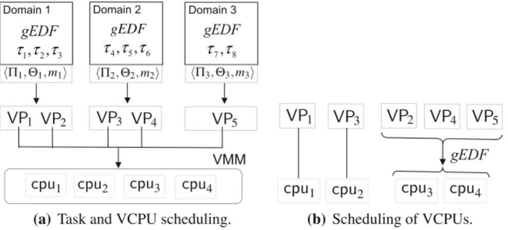
The system we consider consists of multiple real-time components that are scheduled on a multicore virtualization platform, as is illustrated in Fig.1a. Each component corresponds to adomain(virtual machine) of the platform and consists of a set of tasks; these tasks are scheduled on a set of VCPUs by the domain’s scheduler. The VCPUs of the domains are then scheduled on the physical cores by the virtual machine monitor (VMM).

Each taskτiwithin a domain is an explicit-deadline periodic task, defined byτi = (pi,ei,di), where pi is the period,ei is the worst-case execution time (WCET), and di is the relative deadline ofτi. We require that 0<ei ≤di ≤ pifor allτi.

Each VCPU is characterized byVPj =(j, j), wherejis the VCPU’s period andjis the resource budget that the VCPU services in every period, with 0≤j ≤ qj. We say thatVPj is afullVCPU ifj =j, and apartialVCPU otherwise. We assume that each VCPU is implemented as a periodic server (Sha et al.1986) with periodj and maximum budget timej. The budget of a VCPU is replenished at the beginning of each period; if the budget is not used when the VCPU is scheduled to run, it is wasted. We assume that each VCPU can execute only one task at a time. Like in most real-time scheduling research, we follow the conventional real-time task model in which each task is a single thread in this work; an extension to parallel task models is an interestin g but also challenging research direction, which we plan to investigate in our future work.

We assume that all cores are identical and have unit capacity, i.e., each core provides t units of resource (execution time) in any time interval of lengtht. Each core has a private cache,2 all cores share the same memory, and the size of the memory is sufficiently large to ensure that all tasks (from all domains) can reside in memory at the same time, without conflicts.

2.1 Scheduling of tasks and VCPUs

We consider a hybrid version of the earliest deadline first (EDF) strategy. As is shown in Fig.1, tasks within each domain are scheduled on the domain’s VCPUs under the global EDF (gEDF) (Baruah and Baker2008) scheduling policy. The VCPUs of all the domains are then scheduled on the physical cores under a semi-partitioned EDF policy: each full VCPU is pinned (mapped) to a dedicated core, and all the partial VCPUs are scheduled on the remaining cores under gEDF. In the example from Fig.1b,VP1 andVP3 are full VCPUs, which are pinned to the physical cores cpu1 andcpu2, respectively. The remaining VCPUs are partial VCPUs, and are therefore scheduled on the remaining cores under gEDF.

2.2 Cache-related overhead

When two code sections are mapped to the same cache set, one section can evict the other section’s cache blocks from the cache, which causes a cache miss when the former resumes. If the two code sections belong to the same task, this cache miss is an intrinsiccache miss; otherwise, it is an extrinsiccache miss (Basumallick and Nilsen1994). The overhead due to intrinsic cache misses of a task can typically be statically analyzed based solely on the task; however, extrinsic cache misses depend on the interference between tasks during execution. In this paper, we assume that the tasks’ WCETs already include intrinsic cache-related overhead, and we will focus on the extrinsic cache-related overhead. In the rest of this paper, we use the term ‘cache’ to refer to ‘extrinsic cache’.

We usecrpmd_τi to denote the maximum time needed to re-load all the useful cache

blocks (i.e., cache blocks that will be reused) of a preempted taskτi when that task resumes (either on the same core or on a different core).3

Since the overhead for reloading the cache content of a preempted VCPU (i.e., a periodic server) upon its resumption is insignificant compared to the task’s, we will assume here that it is either zero or is already included in the overhead due to cache misses of the running task inside the VCPU.

2 _{In this work, we assume that the cores either do not share a cache, or that the shared cache has been}

partitioned into cache sets that are each accessed exclusively by one core (Kim et al.2012) We believe that an extension to shared caches is possible, and we plan to consider it in our future work.

3 _{We are aware that using a constant maximum value to bound the cache-miss overhead of a task may be}

conservative, and extensions to a finer granularity, e.g., using program analysis, may be possible. However, as the first step, we keep this assumption to simplify the analysis in this work, and we defer such extensions to our future work.

2.3 Objectives

In the above setting, our goal is to develop a cache-aware compositional analysis framework for the system. This framework consists of two elements: (1) an interface representation that can succinctly capture the resource requirements of a component (i.e., a domain or the entire system); and (2) an interface computation method for com-puting a minimum-bandwidth cache-aware interface of a component (i.e., an interface with the minimum resource bandwidth that guarantees the schedulability of a compo-nent in the presence of cache-related overhead).

2.4 Assumptions

We assume that (1) all VCPUs of each domain j share a single period j; (2) all j are known a priori; and (3) each j is available to all domains. These assumptions are important to make the analysis tractable. Assumption 1 is equiv-alent to using a time-partitioned approach; we make this assumption to simplify the cache-aware analysis in Sect. 8, but it should be easy to extend the analysis to allow different periods for the VCPUs. Assumption 2 is made to reduce the search space, which is common in existing work (e.g., Easwaran et al. 2009); it can be relaxed by first establishing an upper bound on the optimal period (i.e., the period of the minimum-bandwidth interface) of each domain j, and then searching for the optimal period value based on this bound. Finally, Assumption 3 is nec-essary to determine how often different events that cause cache-related overhead happen (c.f. Sect.6), which is crucial for the cache-aware interface computation in Sects. 7 and8. One approach to relaxing this assumption is to treat the period of the VCPUs of a domain as an input parameter in the computation of the overhead that another domain experiences. Such a parameterized interface analysis approach is very general, but making it efficient remains an interesting open problem for future research. We note, however, that although each assumption can be relaxed, the consequence of relaxing all three assumptions requires a much deeper investiga-tion.

3 Improvement on multiprocessor periodic resource model

Recall that, when representing a platform, a resource model specifies the character-istics of the resource supply that is provided by that platform; when representing a component’s interface, it specifies the total resource requirements of the component that must be guaranteed to ensure the component’s schedulability. The resource pro-vided by a resource modelRcan also be captured by a SBF, denoted bySBFR(t), that specifies the minimum number of resource units thatRprovides over any interval of lengtht.

In this section, we first describe the existing multiprocessor periodic resource (MPR) model (Shin et al.2008), which serves as a basis for our proposed resource model for multicore virtualization platforms. We then present a new SBF for the MPR model that improves upon the original SBF given in Shin et al.2008, thus enabling tighter MPR-based interfaces for components and more efficient use of resource.

(a)

(b)

Fig. 2 Worst case resource supply of MPR model 3.1 Background on MPR

An MPR model=(,˜ ,˜ m)specifies that a multiprocessor platform with a number of identical, unit-capacity CPUs provides˜ units of resources in every period of˜ time units, with concurrency at mostm(in other words, at any time instant at most m physical processors are allocated to this resource model), where˜ ≤ m˜. Its resource bandwidth is given by/˜ ˜.

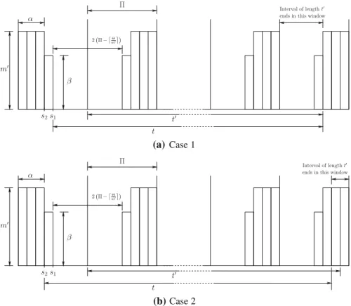
The worst-case resource supply scenario of the MPR model is shown in Fig. 2 (Easwaran et al.2009). Based on this worst-case scenario, the authors in Easwaran et al. (2009) proposed an SBF that bounds the resource supplied by the MPR model =(,˜ ,˜ m), which is defined as follows:

˜ SBF(t)= ⎧ ⎪ ⎨ ⎪ ⎩ 0, ift<0 t/˜˜ +max{0,mx−(m˜ − ˜)}, ift≥0∧ x∈ [1,y] t/˜˜+max{0,mx−(m˜ − ˜)}−(m−β), ift≥0∧x∈ [/ 1,y] (1) whereα = _˜ m , β = ˜−mα, t = t− ˜ −˜ m , x =t− ˜ t ˜ and y= ˜− _˜ m .

3.2 Improved SBF of the MPR model

We observe that, although the function SBF˜ given in Eq. (1) is a valid SBF for the MPR model, it is conservative. Specifically, the minimum amount of resource provided byover a time window of lengtht (see Fig.2) can be much larger than

˜

SBF(t)when (i) the resource bandwidth ofis equal to its maximum concurrency level (i.e.,/˜ ˜ =m), or (ii)x ≤1, wherexis defined in Eq. (1). We demonstrate these cases using the two examples below.

Example 1 Let1= ˜,,˜ m, where˜ = ˜m, andandmare any two positive integer values. By the definition of the MPR model,1represents a multiprocessor platform with exactly m identical, unit-capacity CPUs that are fully available. In other words,1providesmt time units in everyt time units. However, according to Eq. (1), we haveα= _˜ m = ˜,β = ˜−mα =0,t =t − ˜ −m˜ =t, x=t− ˜ t ˜ , andy= ˜− _˜

m =0. Wheneverx∈ [/ 1,y], for allt =t≥0,

˜

SBF₁(t)=t/˜˜ +max{0,mx−(m˜ − ˜)} −(m−β)=mt−m. As a result,SBF˜ ₁(t) <mtfor all for alltsuch thatx∈ [/ 1,y].

Example 2 Let2 = =20, =181,m = 10and considert = 21.1. From Eq. (1), we obtainα =18,β =1,t =t −1 =20.1,x =0.1, and y =2. Since x∈ [/ 1,y], we have ˜ SBF₂(t)= t ˜ ˜ +max{0,mx−(m˜ − ˜)} −(m−β) = 20.1 20 181+max{0,10×0.1−(10×20−181)}−(10−1)=172. We reply on the worst-case resource supply scenario of the MPR model shown in Fig.2to compute the worst-case resource supply of2during a time interval of length t. We first compute the worst-case resource supply whent=21.1 based on Case 1 in Fig.2:

– tstarts at the time points1;

– During the time interval[s1,s1+(˜ −α−1)], i.e.,[s1,s1+1],2supplies 0 time unit;

– During the time interval[s1+(˜−α−1),s1+(˜−α−1)+ ˜], i.e.,[s1+1,s1+21], 2supplies=181 time units;

– During the time interval[s1+(˜ −α−1)+,s1+t], i.e.,[s1+21,s1+21.1], 2supplies 0 time unit.

Therefore,2supplies 181 time units during a time interval of lengtht =21.1 based on Case 1 in Fig.2.

Next, we compute the worst-case resource supply whent=21.1 based on Case 2 in Fig.2:

– tstarts at the time points2;

– During the interval[s2,s2+(˜ −α)], i.e.,[s2,s2+2]suppliesβ=1 time unit; – During the interval[s2+(˜ −α),s2+2(˜ −α)], i.e.,[s2+2,s2+4],supplies

β=1 time unit;

– During the interval[s2+2(˜ −α),s2+t], i.e.,[s2+4,s2+21.1],supplies (21.1−4)×m=171 time units.

Therefore,2supplies 1+1+171 = 173 time units during any time interval of lengtht based on Case 2 in Fig.2. Because the two cases in Fig.2are the only two possible worst-case scenarios of the MPR resource model (Easwaran et al.2009), the worst-case resource supply of2during any time interval of lengtht =21.1 is 173 time units. SinceSBF2(t)=172, the value computed by Eq. (1) under-estimates the actual resource provided by2.

Based on the above observations, we introduce a new SBF that can better bound the resource supply of the MPR model. This improved SBF is computed based on the worst-case resource supply scenarios shown in Fig.2.

Lemma 1 The amount of resource provided by the MPR model= ˜,,˜ mover any time interval of length t is at leastSBF(t), where

SBF(t)= ⎧ ⎪ ⎪ ⎪ ⎪ ⎨ ⎪ ⎪ ⎪ ⎪ ⎩ 0, t<0 t ˜ _˜ +max0,mx−(m˜ − ˜), t≥0 ∧x∈ [1−_mβ,y] max0, βt−2(˜ − _m˜) t∈ [0,1] ∧x∈ [1−mβ,y] t ˜ ˜+max 0,mx−(m˜ − ˜)−(m−β), t≥1∧ x∈ [1−_mβ,y] (2) where α= ˜ m ;β= ˜ −mα, ˜ =m m, ˜ =m; t _=t− ˜ − ˜ m ; t=t−1; x= t− ˜ t ˜ ;x= t− ˜ t ˜ +1; y= ˜− ˜ m .

Proof We will prove that the functionSBF(t)is a valid SBF of based on the worst-case resource supply patterns ofshown in Fig.2.

Consider the time interval of lengtht (called time intervalt) and the black-out interval (during which the resource supply is zero) in Fig.2. By definition,x is the remaining time of the time intervaltin the last period of, and yis half the length of the black-out interval plus one. There are four cases ofx, which determine whether SBF(t)corresponds to the resource supply ofin Case 1 or Case 2 in Fig.2:

– x∈ [1,y]: It is easy to show that the value ofSBF(t)in Case 1 is no larger than its value in Case 2. Note that if we shift the time interval of lengtht in Case 1 by one time unit to the left, we obtain the scenario in Case 2. In doing so,SBF(t)will

be increased byβtime units from the first period but decreased by at mostβ time units from the last period. Therefore, the pattern in Case 2 supplies more resource than the pattern in Case 1 whenx∈ [1,y].

– x∈ [1−_mβ,1]: As above, if we shift the time interval of lengthtin Case 1 by one time unit to the left, we obtain the scenario in Case 2. Recall thatxis the remaining time of the time interval of lengtht in the last period, x ≤ 1 and y ≥ 1. In shifting the time interval of lengtht,SBF(t)will lose(1−x)mtime units while gainingβtime units from the first period. Becausex≥1−_mβ,β−(1−x)m≥0. Therefore,SBF(t)gainsβ−(1−x)m≥0 time units in transferring the scenario in Case 1 to the scenario in Case 2. Hence, Case 1 is the worst-case scenario when x∈ [1−_mβ,1].

– x∈ [0,1−_mβ): It is easy to show thatsupplies less resource in Case 2 than in Case 1 when we shift the time interval of lengthtof Case 1 to left by one time unit to get Case 2. Therefore, Case 2 is the worst-case scenario whenx∈ [0,1−_mβ]. – x > y: We can easily show thatSBF(t)is no larger in Case 2 than in Case 1. Becausex>y, when we shift the time intervaltof Case 1 to left by one time unit to get the scenario in Case 2,losesmtime units from the last period but only gainsβ time units, whereβ ≤ m. Therefore, Case 2 is the worst-case scenario whenx>y.

From the above, we conclude that Case 1 is the worst-case resource supply scenario whenx ∈ [1−_mβ,y], and Case 2 is the worst-case resource supply scenario when x∈ [1−_mβ,y].

Based on the worst-case resource supply scenario under different conditions above, we can derive Eq.2as follows:

– Whent < 0: It is obvious thatSBF(t)=0 becausesupplies no resource in the black-out interval.

– Whent≥0 andx∈ [1−_mβ,y]: Based on the worst-case resource supply scenario in Case 1,has t_˜

periods and provides˜ time units in each period.hasx remaining time in the last period, which provides max{0,mx−(m−)−(m− β)}time units. Therefore,supplies t_˜ ˜+max{0,mx−(m−)−(m−β)} time units during time intervalt.

– Whent ∈ [0,1]andx ∈ [1−_mβ,y]: Becauset ∈ [0,1],t ∈ [− m˜, −

m˜ +1]. Therefore,t<2(− ˜ m)+2, where 2(− ˜

m)is the length of the black-out interval. Hence, the worst-case resource supply ofduring time interval tis max{0, β(t−2(− _m))}.

– When t > 1 and x ∈ [1− _mβ,y], the worst-case resource supply scenario is Case 2.has t_˜periods and provides˜ time units in each period.supplies max{0,mx−(m˜ − ˜)−(m−β)}time units during its first and last periods. Therefore,SBF(t)= t_˜+max{0,mx−(m˜ − ˜)−(m−β)}. The lemma follows from the above results.

It is easy to verify that, under the two scenarios described in Examples1 and2, SBF (t)and SBF (t) correspond to the actual minimum resource that and

2 provide, respectively. It is also worth noting that, for the scenario described in Example1, the compositional analysis for the MPR model Easwaran et al. (2009) is compatible4 with the underlying gEDF schedulability test under the improved SBF but not under the original SBF in Eq. (1). In the next example, we further demonstrate the benefits of the improved SBF in terms of resource bandwidth saving.

Example 3 Consider a component C with a taskset τ = {τ1 = · · · = τ4 = (200,100,200)}that is scheduled under gEDF, and the period of the MPR inter-face ofCis fixed to be 40. Following the interface computation method in Easwaran et al. (2009), the corresponding minimum-bandwidth MPR interfaces,1and2, ofC when using the original SBF in Eq. (1) and when using the improved SBF in Eq. (2) are obtained as follows:1 = 40,145,4and2= 40,120,3. Thus, the MPR inter-face ofCcorresponding to the improved SBF can save 145/40−120/40=0.625 cores compared to the interface corresponding to the original SBF proposed in Easwaran et al. (2009).

4 Deterministic multiprocessor periodic resource model

In this section, we introduce the deterministic multiprocessor resource model (DMPR) for representing the interfaces. The MPR model described in the previous section is simple and highly flexible because it represents the collective resource requirements of components without fixing the contribution of each processor a priori. However, this flexibility also introduces some extra overhead: it is possible that all processors stop providing resources at the same time, which results in a long worst-case starvation interval (it can be as long as 2(˜ − ˜/m) time units (Easwaran et al.2009). Therefore, to ensure schedulability in the worst case, it is necessary to provide more resources than strictly required. However, we can minimize this overhead by restricting the supply pattern of some of the processors. This is a key element of the deterministic MPR that we now propose.

A DMPR model is a deterministic extension of the MPR model, in which all of the processors but one always provide resource with full capacity. It is formally defined as follows.

Definition 1 A DMPR μ= , ,m specifies a resource that guaranteesm full (dedicated) unit-capacity processors, each of which providest resource units in any time interval of lengtht, and one partial processor that providesresource units in every period oftime units, where 0≤ < andm≥0.

By definition, the resource bandwidth of a DMPRμ= , ,misbw_μ=m+. The total number of processors ofμism_μ=m+1, if >0, andm_μ=m, otherwise. Observe that the partial processor ofμis represented by a single-processor periodic resource model =(, )(Shin and Lee2003). (However, it can also be represented

4 _{We say that a compositional analysis method is compatible with the underlying component’s}

schedula-bility test it uses if whenever a componentCwith a tasksetτ is deemed schedulable onmcores by the schedulability test, thenCis also deemed schedulable under an interface with bandwidth no larger thanm by the compositional analysis method.

VP1 Θ Θ Θ VP2 VP3 2Π Π 3Π 0 t

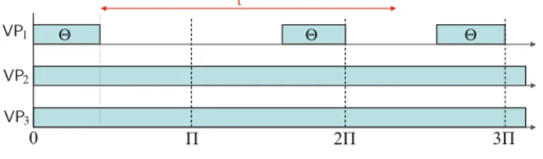
Fig. 3 Worst-case resource supply pattern ofμ= , ,m

by any other single processor resource model, such as EDP model Easwaran et al. 2007.) Based on this characteristic, we can easily derive the worst-case supply pattern ofμ(shown in Fig.3) and its SBF, which is given by the following lemma:

Lemma 2 The SBF of a DMPR modelμ= , ,mis given by: SBF_μ(t)=

mt, if=0 ∨ (0≤t≤−)

mt+y+max{0,t−2(−)−y},otherwise where y=t−(−), for all t > −.

Proof Consider any interval of lengtht. Since the full processors ofμare always avail-able,μprovides the minimum resource supply iff the partial processor provides the worst-case supply. Since the partial processor is a single-processor periodic resource model =(, ), its minimum resource supply in an interval of lengtht is given by Shin and Lee (2003):SBF (t) =0, if = 0 or 0 ≤ t ≤ −; otherwise, SBF (t)=y+max{0,t−2(−)−y}wherey=t−(−). In addition, the mfull processors ofμprovides a total ofmtresource units in any interval of lengtht. Hence, the minimum resource supply ofμin an interval of lengthtismt+SBF (t).

This proves the lemma.

It is easy to show that, when a DMPR μ and an MPR have the same period, bandwidth, and total number of processors, thenSBF_μ(t)≥SBF(t)for allt ≥0, and the worst-case starvation interval ofμis always shorter than that of.

5 Overhead-free compositional analysis

In this section, we present our method for computing the minimum-bandwidth DMPR interface for a component, assuming that the cache-related overhead is negligible. The overhead-aware interface computation is considered in the next sections. We first recall some key results for components that are scheduled under gEDF (Easwaran et al.2009).

5.1 Component schedulability under gEDF

The demand of a taskτi in a time interval[a,b]is the amount of computation that must be completed within[a,b]to ensure that all jobs ofτ with deadlines within

[a,b]are schedulable. Whenτi =(pi,ei,di)is scheduled under gEDF, its demand in any interval of lengthtis upper bounded by Easwaran et al. (2009):

dbfi(t)= _t+(p i−di) pi ei+CIi(t),where CIi(t)=min ei,max 0,t− _{t+(pi −di)} pi pi . (3)

In Eq. (3),CIi(t)denotes the maximum carry-in demand ofτi in any time interval

[a,b] withb−a = t, i.e., the maximum demand generated by a job ofτi that is released prior toabut has not finished its execution requirement at timea.

Consider a componentC with a tasksetτ = {τ1, . . . τn}, whereτi =(pi,ei,di), and suppose the tasks inCare schedulable under gEDF by a multiprocessor resource withm processors. From Easwaran et al. (2009), the worst-case demand ofC that must be guaranteed to ensure the schedulability ofτk in a time interval(a,b], with b−a=t ≥dkis bounded by: DEM(t,m)=mek+ τi∈τ ˆ Ii,2+ i:i∈L_(m−1) (I¯i,2− ˆIi,2) (4) where Iˆi,2=min dbfi(t)−CIi(t), t−ek , ∀i =k, ˆ Ik,2=min dbfk(t)−CIk(t)−ek, t−dk ; ¯ Ii,2=min dbfi(t), t−ek , ∀i =k, ¯ Ik,2=min dbfk(t)−ek, t−dk ;

andL₍m−1) is the set of indices of all tasksτi that haveI¯i_,2− ˆIi_,2being one of the (m−1)largest such values for all tasks.5This leads to the following schedulability test forC:

Theorem 1 (Easwaran et al.2009)A component C with a task setτ = {τ1, . . . τn}, where τi = (pi,ei,di), is schedulable under gEDF by a multiprocessor resource model R with mprocessors in the absence of overhead if, for each taskτk ∈τ and for all t ≥ dk,DEM(t,m)≤ SBFR(t), whereDEM(t,m)is given by Eq.(4)and SBFR(t)gives the minimum total resource supply by R in an interval of length t .

5.2 DMPR interface computation

In the absence of cache-related overhead, the minimum resource supply provided by a DMPR modelμ= , ,min any interval of lengthtisSBF_μ(t), which is given by Lemma2. Since each domain schedules its tasks under gEDF, the following theorem follows directly from Theorem1.

5 _Here,d

Theorem 2 A domainDwith a task setτ = {τ1, . . . τn}, whereτi =(pi,ei,di), is schedulable under gEDF by a DMPR modelμ=(, ,m)if, for eachτk ∈τ and for all t≥dk,

DEM(t,m_μ)≤SBF_μ(t), (5) where mμ=m+1if >0, and mμ=m otherwise.

We say that μ is a feasible DMPR forD if it guarantees the schedulability of D according to Theorem2.

The next theorem derives a bound of the valuetthat needs to be checked in Theo-rem2.

Theorem 3 If Eq.(5)is violated for some value t , then it must also be violated for a value that satisfies the condition

t< C+mμek+U+B +m−UT

(6)

where Cis the sum of the m_μ−1largest ei; U = ni=1(pi−di)e_pi

i; UT = n i=1 ei pi; and B =2(−).

Proof The proof follows a similar line with the proof of Theorem 2 in Easwaran et al. (2009). Recall thatDEM(t,m_μ)is given by Eq. (4). According to Eq. (4), we have

ˆ Ii,2≤ t+(pi−di) pi ei ≤ t+(pi −di) pi ei ≤t ei pi + pi−di pi ei. Therefore, n i=1 ˆ Ii,2≤ n i=1 tei pi + n i=1 pi−di pi ei =tUT +U.

Because the carry-in workload ofτiis no more thanei, we derive

i:i∈L₍m_μ−1)

(I¯i,2− ˆIi,2)

≤C. Thus,

DEM(t,m_μ)≤m_μek+tUT +U+C.

Further, SBF_μ(t) gives the worst-case resource supply of the DMPR model μ= , ,mover any interval of lengtht. Based on Lemma2, the resource

sup-ply ofμ is total resource supply of one partial VCPU(, ) andm full VCPUs. From (Shin and Lee2003), the resource supply of the partial VCPU(, )over any interval of lengthtis at least(t−2(−)). In addition, the resource supply ofm full VCPUs over any interval of lengthtismt. Hence, the resource supply ofμover any interval of lengtht is at leastmt+(t−2(−)). In other words,

SBF_μ(t)≥mt+

(t−2(−)).

Suppose Eq. (5) is violated, i.e.,DEM(t,m_μ) >SBF_μ(t)for some valuet. Then, combine with the above results, we imply

m_μek+tUT +U+C>mt+ (t−2(−)), which is equivalent to t <C+mμek+U+B +m−UT .

Hence, if Eq. (5) is violated for some valuet, thentmust satisfy Eq. (6). This proves

the theorem.

The next lemma gives a condition for the minimum-bandwidth DMPR interface with a given period.

Lemma 3 A DMPR model μ∗ = , ∗,m∗ is the minimum-bandwidth DMPR with periodthat can guarantee the schedulability of a domainDonly if m∗≤m for all DMPR modelsμ= , ,mthat can guarantee the schedulability of a domain

D.

Proof Supposem∗ > m for some DMPR μ = , ,m. Then, m∗ ≥ m+1 and, hence, bw_μ∗ = m∗ +∗/ ≥ m+1+∗/ ≥ m+1. Since < , bw_μ=m+/ <m+1. Thus,bw_μ∗>bw_μ, which implies thatm∗cannot be the minimum-bandwidth DMPR with period. Hence the lemma. 5.3 Computing the domains’ interfaces

LetDi be a domain in the system andi be its given VCPU period (c.f. Sect. 2). The minimum-bandwidth interface ofDi with periodi is the minimum-bandwidth DPRM modelμi = i, i,mi that is feasible forDi. To obtainμi, we perform binary search on the number of full processorsm_i, and, for each valuem_i, we compute the smallest value of_isuch that_i, i,m_iis feasible forDi (using Theorem2).6

6 _{Note that the number of full processors is always bounded from below by U}

i, whereUi is the total utilization of the tasks inDi, and bounded from above by the number of tasks inDi or the number of physical platform (if given), whichever is smaller.

Thenmi is the smallest value ofm_ifor which a feasible interface is found, and,iis the smallest budget_i computed formi.

5.4 Computing the system’s interface

The interface of the system can be obtained by composing the interfacesμi of all domainsDiin the system under the VMM’s semi-partitioned EDF policy (c.f. Sect.2). LetDdenote the number of domains of the platform.

Observe that each interfaceμi = i, i,mican be transformed directly into an equivalent set ofmi full VCPUs (with budgeti and periodi) and, ifi > 0, a partial VCPU with budgeti and periodi. LetCbe a component that contains all the partial VCPUs that are transformed from the domains’ interfaces. Then the VCPUs inCare scheduled together under gEDF, whereas all the full VCPUs are each mapped to a dedicated core.

Since each partial VCPU inCis implemented as a periodic server, which is essen-tially a periodic task, we can compute the minimum-bandwidth DMPR interface μC = C, C,mCthat is feasible forCby the same technique used for domains. Combiningμ_Cwith the full VCPUs of the domains, we can see that the system must be guaranteedm_C+ _1≤i≤Dmifull processors and a partial processor, with budgetC and period_C, to ensure the schedulability of the system. The next theorem directly follows from this observation.

Theorem 4 Letμi = i, i,mibe the minimum-bandwidth DMPR interface of domainDi, for all1≤i ≤ D. LetCbe a component with the taskset

τC = {(i, i, i) | 1≤i ≤ D ∧ i >0},

which are scheduled under gEDF. Then the minimum-bandwidth DMPR interface with period _C of the system is given by: μsys = C, C,msys, where μC =

C, C,m_Cis a minimum-bandwidth DMPR interface with period _C ofC and msys=mC+ 1≤i≤Dmi.

Based on the system’s interface, one can easily derive the schedulability of the system as follows (the lemma comes directly from the interface’s definition):

Lemma 4 Let M be the number of physical cores of the platform. The system is schedulable if M ≥msys+1, or, M =msysandC=0, whereC, C,msysis

the minimum-bandwidth DMPR system’s interface.

The results obtained above assume that the cache-related overhead is negligible. We will next develop the analysis in the presence of cache-related overhead.

6 Cache-related overhead scenarios

In this section, we characterize the different events that cause cache-related overhead; this is needed for the cache-aware analysis in Sects.7and8.

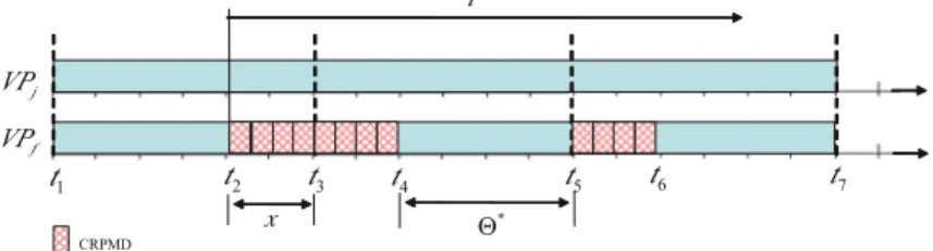
Fig. 4 Cache-related overhead of a task-preemption event

Cache-related overhead in a multicore virtualization platform is caused by (1) task preemption within the same domain, (2) VCPU preemption, and (3) VCPU exhaustion of budget. We discuss each of them in detail below.

6.1 Event 1: task-preemption event

Since tasks within a domain are scheduled under gEDF, a newly released higher-priority task preempts a currently executing lower-higher-priority task of thesamedomain, if none of the domain’s VCPUs are idle. When a preempted task resumes its execution, it may experience cache misses: its cache content may have been evicted from the cache by the preempting task (or tasks with a higher priority than the preempting task, if a nested preemption occurs), or the task may be resumed on a different VCPU that is running on a different core, in which case the task’s cache content may not be present in the new core’s cache. Hence the following definition:

Definition 2 (Task-preemption event) A task-preemption event ofτi is said to occur when a job of another taskτjin the same domain is released and this job can preempt the current job ofτi.

Figure 4 illustrates the worst-case scenario of the overhead caused by a task-preemption event. In the figure, a task-preemption event of τ1 happens at time t = 3 whenτ3is released (and preemptsτ1). Due to this event,τ1experiences a cache miss at timet = 5 when it resumes. Sinceτ1resumes on a different core, all the cache blocks it will reuse have to be reloaded into new core’s cache, which results in cache-related preemption/migration overhead onτ1. (Note that the cache content ofτ1is not necessarily reloaded all at once, but rather during its remaining execution after it has been resumed; however, for ease of exposition, we show the combined overhead at the beginning of its remaining execution).

Since gEDF is work-conserving, tasks do not suspend themselves, and each task resumes at most once after each time it is preempted. Therefore, each taskτk expe-riences the overhead caused by each of its task-preemption events at most once, and this overhead is bounded from above bycrpmd_τk .

Lemma 5 A newly released job ofτjpreempts a job ofτiunder gEDF only if dj <di. Proof Supposedj ≥ di and a newly released job Jj ofτj preempts a job Ji ofτi. Then,Jjmust be released later thanJi. As a result, the absolute deadline ofJjis later

thanJi’s (sincedj ≥di), which contradicts the assumption thatJjpreemptsJiunder

gEDF. This proves the lemma.

The maximum number of task-preemption events in each period ofτi is given by the next lemma.

Lemma 6 (Number of task-preemption events) The maximum number of task-preemption events of τi under gEDF during each period of τi, denoted by N_τ1_i, is bounded by N_τ1_i ≤ τj∈HP(τi) _di−dj pj (7)

whereHP(τi)is the set of tasksτj within the same domain withτi with dj <di. Proof Letτ_icbe the current job ofτi in a period ofτi, and letr_icbe its release time. From Lemma5, only jobs of a taskτj withdj < di and in the same domain can preemptτ_ic. Further, for each suchτj, only the jobs that are released afterτ_icand that have absolute deadlines no later thanτ_ic’s can preemptτ_ic. In other words, only jobs that are released within the interval(r_ic,r_ic+di −dj]can preemptτ_ic. As a result, the maximum number of task-preemption events ofτi under gEDF is no more than

τj∈HP(τi) _d i−dj pj . 6.2 VCPU-preemption event

Definition 3 (VCPU-preemption event) A VCPU-preemption event of VPi occurs whenVPi is preempted by a higher-priority VCPUVPj of another domain.

When a VCPUVPiis preempted, the currently running taskτlonVPimay migrate to another VCPUVPk of the same domain and may preempt the currently running taskτm onVPk. This can cause the tasks running onVPk experiences cache-related preemption or migration overhead twice in the worst case, as is illustrated in the following example.

Example 4 The system consists of three domainsD1–D3.D1has VCPUsVP1(full) and VP2 (partial); D2 has VCPUs VP3 (full) and VP4 (partial); and D3 has one partial VCPUVP5. The partial VCPUs of the domains—VP2(5,3),VP4(8,3)and VP5(6,4)—are scheduled under gEDF oncpu1andcpu2, as is shown in Fig.5a. In addition, domainD2consists of three tasks,τ1(8,4,8),τ2(6,2,6)andτ3(10,1.5,10), which are scheduled under gEDF on its VCPUs (Fig.5b).

As is shown in Fig.5a, a VCPU-preemption event occurs at timet=2, whenVP4 (ofD2) is preempted byVP2. Observe that, withinD2at this instant,τ2is running on VP4andτ1is running onVP3. Sinceτ2has an earlier deadline thanτ1, it is migrated toVP3and preemptsτ1there. SinceVP3is mapped to a different core fromcpu1,τ2 has to reload its useful cache content to the cache of the new core att =2. Further, whenτ1resumes at timet = 3.5, it has to reload the useful cache blocks that may have been evicted from the cache byτ2. Hence, the VCPU-preemption event ofVP4 causes overhead for both of the tasks in its domain.

(a) Schedulingscenario of VCPUs. (b) Cache overhead of tasks inD2. Fig. 5 Cache overhead due to a VCPU-preemption event

Lemma 7 Each VCPU-preemption event causes at most two tasks to experience a cache miss. Further, the cache-related overhead it causes is at most crpmd_C =

max_τi∈Ccrpmdτi , where C is the component that has the preempted VCPU.

Proof At most one task is running on a VCPU at any time. Hence, when a VCPUVPi ofCis preempted, at most one task (τm) onVPi is migrated to another VCPUVPj, and this task preempts at most one task (τl) onVPj. As a result, at most two tasks (i.e.,τm andτl) incur a cache miss because of the VCPU-preemption event. (Note thatτlcannot immediately preempt another taskτnbecause otherwise,τmwould have migrated to the VCPU on whichτnis running and preemptedτninstead.) Further, since the overhead caused by each cache miss inCis at mostcrpmd_C =max_τi∈C

crpmd

τi ,

the maximum overhead caused by the resulting cache misses is at most 2crpmd_C . Since the partial VCPUs are scheduled under gEDF as implicit-deadline tasks (i.e., the task periods are equal to their relative deadlines), the number of VCPU-preemption events of a partial VCPUVPi during eachVPi’s period also follows Lemma6. The next lemma is implied directly from this observation.

Lemma 8 (Number of VCPU-preemption events)LetVPi =(i, i)for all partial VCPUsVPiof the domains. LetHP(VPi)be the set ofVPjwith0< j<j < i. Denote by N_VP2

i and N

2

VPi,τk the maximum number of VCPU-preemption events of

VPi during each period ofVPi and during each period ofτk insideVPi’s domain, respectively. Then, N_VP2 _i ≤ VPj∈HP(VPi) i−j j (8) N_VP2 i,τk ≤ VPj∈HP(VPi) _p k j . (9)

6.3 VCPU-completion event

Definition 4 (VCPU-completion event) A VCPU-completion event ofVPi happens whenVPi exhausts its budget in a period and stops its execution.

Like in VCPU-preemption events, each VCPU-completion event causes at most two tasks to experience a cache miss, as given by Lemma9.

Lemma 9 Each VCPU-completion event causes at most two tasks to experience a cache miss.

Proof The effect of a completion event is very similar to that of a VCPU-preemption event. WhenVPifinishes its budget and stops, the running taskτmonVPi may migrate to another running VCPUVPj, and,τm may preempt at most one task τl onVPj. Hence, at most two tasks incur a cache miss due to a VCPU-preemption

event.

Lemma 10 (Number of VCPU-completion events)Let N_VP3

i and N

3

VPi,τkbe the

num-ber of VCPU-completion events ofVPi in each period ofVPi and in each period of τkinsideVPi’s domain. Then,

N_VP3 _i ≤1 (10) N_VP3 _i,τk ≤ _p k−i i +1 (11)

Proof Eq. (10) holds becauseVPicompletes its budget at most once every period. Fur-ther, observe thatτi experiences the worst-case number of VCPU-preemption events when (1) its period ends at the same time as the budget finish time ofVPi’s current period, and (2)VPifinishes its budget as soon as possible (i.e.,Bitime units from the beginning of the VCPU’s period) in the current period and as late as possible (i.e., at the end of the VCPU’s period) in all its preceding periods. Eq. (11) follows directly

from this worst-case scenario.

6.4 VCPU-stop event

Since a VCPU stops its execution when its VCPU-completion or VCPU-preemption event occurs, we define aVCPU-stop eventthat includes both types of events. That is, a VCPU-stop event ofVPioccurs whenVPistops its execution because its budget is fin-ishedorbecause it is preempted by a higher-priority VCPU. Since VCPU-stop events include both VCPU-completion events and VCPU-preemption events, the maximum number of VCPU-stop events of VPi during eachVPi’s period, denoted as N_VPstop

i , satisfies N_VPstop i =N 2 VPi +N 3 VPi ≤ VPj∈HP(VPi) _i−j j +1 (12)

6.5 Overview of the overhead-aware compositional analysis

Based on the above quantification, in the next two sections we develop two different approaches, task-centric and model-centric, for the overhead-aware interface compu-tation. Although the obtained interfaces by both approaches are safe and can each be used independently, we combine them to obtain the interface with the smallest bandwidth as the final result.

7 Task-centric compositional analysis

This section introduces two task-centric analysis methods to account for the cache-related overhead in the interface computation. The first, denoted asbaseline, accounts for the overhead by inflating the WCET of every task in the system with the maximum overhead it experiences within each of its periods. The second, denoted as task-centric- ub, combines the result of the first method using an upper bound on the number of VCPUs that each domain needs in the presence of cache-related overhead. We describe each method in detail below.

7.1BASELINE: analysis based on WCET-inflation

As was discussed in Sect.6, the overhead that a task experiences during its lifetime is composed of the overhead caused by task-preemption events, VCPU-preemption events and VCPU-completion events. In addition, when one of the above events occurs, each taskτkexperiences at most one cache miss overhead and, hence, a delay of at most

crpmd

τk . From (Brandenburg2011), the cache overhead caused by a task-preemption

event can be accounted for by inflating the higher-priority taskτiof the event with the maximum cache overhead caused byτi. From Lemmas8and10, we conclude that the maximum overheadτkexperiences within each period is

δcrpmd τk =_τ max i∈LP(τk) {crpmd τi } + crpmd τk (N 2 VPi,τk+N 3 VPi,τk

whereLP(τk)is the set of tasksτi within the same domain withτkwithdi >dk and VPi is the partial VCPU of the domain ofτk. As a result, the worst-case execution time ofτkin the presence of cache overhead is at most

ek=ek+δcrpmd_τk . (13)

Thus, we can state the following theorem:

Theorem 5 A component with a tasksetτ = {τ1, . . . τn}, whereτk = (pk,ek,dk), is schedulable under gEDF by a DMPR modelμ in the presence of cache-related overhead if its inflated tasksetτ = {τ₁, . . . τn}is schedulable under gEDF byμin the absence of cache-related overhead, whereτ_k =(pk,e_k,dk), and e_k is given by Eq.13.

Based on Theorem5, we can compute the DMPR interfaces of the domains and the system by first inflating the WCET of each taskτkin each domain with the overhead

δcrpmd

τk and then applying the same method as the overhead-free interface computation

in Sect.5.2.7

7.2TASK-CENTRIC-UB: Combination ofBASELINEwith an upper bound on the number of VCPUs

Recall from Sect. 6 that, VCPU-preemption events and VCPU-completion events happen only when the component has a partial VCPU. Therefore, the taskset in a component with no partial VCPU experiences only the cache overhead caused by task-preemption events. Recall that when a task-preemption event happens, the cor-responding lower-priority taskτi experiences a cache miss delay of at mostcrpmd_τi .

Thus, the maximum cache overhead that a high-priority task τk causes to any pre-empted task is max_τi∈LP(τk)

crpmd

τi , where LP(τk)is the set of tasksτi within the

same domain withτkthat havedi >dk. As a result, the worst-case execution time of τkin the presence of cache overhead caused by task-preemption events is at most

e_k =ek+ max τi∈LP(τk)

crpmd

τi , (14)

whereτi ∈LP(τk)ifdi >dk. This implies the following lemma:

Lemma 11 A component with a tasksetτ = {τ1, . . . , τn}, whereτk=(pk,ek,dk), is schedulable under gEDF by a DMPR modelμ¯ = ,0,m¯in the presence of cache-related overhead if its inflated tasksetτ= {τ₁, . . . , τ_n}is schedulable under gEDF by μ_{= , ,min the absence of cache-related overhead, whereτ}

k =(pk,ek,dk), e_k is given by Eq.14, andm¯ = m+ . Further, the maximum number of full VCPUs of the interface of the tasksetτ in the presence of cache overhead ism.¯ Proof First, observe that the inflated tasksetτsafely accounts for all the cache over-head experienced byτ. This is because

(1) inflating the worst-cache execution time of each taskτkwith maxτi∈LP(τk) crpmd

τi

is safe to account for the cache overhead delay caused by task-preemption events (as was proven in Brandenburg2011), and

(2) the DMPR modelμ¯ has no partial VCPU and thus,τ does not experience any cache overhead caused by VCPU-preemption events or VCPU-completion events. Further, based on Lemma2, one can easily show that the resource SBFSBF_μ(t) of a DMPR modelμ = , ,m is monotonically non-decreasing with the budget ofμwhen the period ofμis fixed. In other words,SBF_μ¯(t)≥SBF_μ(t) for allt. Combine the above observations, we imply thatτ is schedulable under the resource modelμ¯in the presence of cache overhead ifτis schedulable under

7 _{Note that we inflate only the tasks’ WCETs and not the VCPUs’ budgets, sinceδ}crpmd

τk includes the overhead for reloading the useful cache content of a preempted VCPU when it resumes.

the resource modelμin the absence of cache overhead. This proves the first part of the lemma.

Sinceτis schedulable under the resource modelμ¯in the presence of cache overhead, the number of full VCPUs of the overhead-aware interface ofτ is always less than or equal to the ceiling of the bandwidth ofμ¯, which is exactlym.¯ Note that the maximum number of full VCPUs given by Lemma11can be larger or smaller than the interface bandwidth computed by the baseline method, as is illustrated in the following two examples.

Example 5 Consider a system Sys1 consisting of two domains, C1 and C2, with workloadsτC1 = {τ

1

1 = · · · =τ13 =(100,40,100)}andτC2 = {τ

1

2 = · · · =τ23=

(100,40,100)}, respectively. Suppose thatSys1employs the hybrid EDF scheduling strategy described in Sect.2; the periods of DMPR interfaces of C1,C2andSys1 are set to 80,40 and 20, respectively; and the cache overhead per task is 1. Then, the DMPR cache-aware interface of C1 computed using the baseline method is μC1 = 80,76,1, which has a bandwidth of 1+76/80=1.95.

In contrast, if we only consider the cache overhead caused by task-preemption events, then the interface of the system is given by μ_C1 = 80,64,1. Based on Lemma11, the maximum number of full VCPUs ofC1is 1+64/80 = 2, and the corresponding DMPR interface isμ¯C1 = 80,0,2. Thus, the interface computed by thebaselinemethod has a smaller bandwidth than the maximum number of full

VCPUs given by Lemma11.

Example 6 Consider a systemSys₂that is identical to the systemSys₁in Example5, except that the cache overhead for each task is 5 instead of 1. In this case, the cache-aware interface ofC1computed using thebaselinemethod isμ¯C1 = 80,72,2, which has a bandwidth of 2+72/80=2.9. In contrast, if we only consider only the cache overhead caused by task-preemption events, then the interface of the system is given byμ_C

1 = 80,74,1. Based on Theorem11, the maximum number of full VCPUs is 1+74/80=2. Therefore, the interface computed by thebaselinemethod has a larger bandwidth than the maximum number of full VCPUs given by Lemma11. Since the interfaceμ¯given by Lemma11does not always have a smaller bandwidth than the interface computed using thebaseline method, we combine the two

inter-faces to derive the minimum-bandwidth DMPR interface in the presence of overhead, as is given by Theorem6. The correctness of this theorem is derived directly from the correctness of Lemma11and Theorem5.

Theorem 6 Let C be a component with a tasksetτ = {τ1, . . . , τn}that is schedu-lable by the gEDF scheduler, whereτk = (pk,ek,dk)for all1 ≤ k ≤ n. Suppose μ

C = , ,mis the feasible DMPR interface given by Theorem5, and mis the maximum number of full VCPUs of C given by Lemma11. Then, the component C is schedulable under the DMPR interfaceμC, whereμC =μ_C if m >m+

, and μC = ,0,motherwise.

Interface computation under thetask- centric- ubmethodBased on the above results, the overhead-aware interface for a system can be obtained by first computing

the interface for each domain using Theorem 6, and then computing the system’s interface by applying the overhead-free interface computation in Sect.5.

7.3TASK-CENTRIC-UBversusBASELINE

As was discussed in Sect.7.2, the interface of a domain computed by the task-centric- ub method always has a bandwidth no larger than the bandwidth of the

interface computed by thebaselinemethod.

We will show that this relationship also holds for the interfaces at the system level. We first define the dominance relation between any two analysis methods as follows: Definition 5 A compositional analysis methodC S Ais said to dominate another com-positional analysis methodC S A iff for any systemS, the interface bandwidth of S when computed usingC S Ais always less than or equal to the interface bandwidth of Swhen computed usingC S A.

Lemma 12 Thetask- centric- ubmethod always dominates thebaselinemethod. Proof Consider a systemSwithDdomains,{C1, . . . ,CD}. LetμCi = i, i,mi

andμ_C

i = i,

i,mibe the minimum-bandwidth DMPR interfaces ofCi under thetask- centric- ubmethod and thebaselinemethod, respectively. We have the

following:

– Under the task- centric- ubmethod, the system has a set of partial VCPUs, VPpart = {VP1 = (1, 1), . . . ,VPD = (D, D)}, and (m1+ · · · +mD) full VCPUs. Based on the analysis in Sect.5, the minimum-bandwidth DMPR interface ofSis given byμS= C, C,mS, whereμC = C, C,mCis the minimum-bandwidth DMPR interface forVPpartandmS=mC+ 1_≤i_≤Dmi. – Under thebaseline method, the system has a set of partial VCPUs,VPpart =

{VP₁ = (1, 1), …,VPD = (D, D)}and(m1+ · · · +mD)full VCPUs. Therefore, the minimum-bandwidth DMPR interface system is given byμ_S =

C, _C,m_S, where μ_C = , _C,m_C is the minimum-bandwidth DMPR interface of the partial VCPU setVP_part, andm_S=m_C + 1_≤i_≤Dmi.

From Theorem6, there are two cases for the relationship betweenμCi andμCi:

1. i = _i andmi = m_i, if the interface bandwidth computed by thebaseline

method is less than or equal to the maximum number of full VCPUs ofCi given by Lemma11(i.e.,m_i+i

≤mi+i); 2. i =0 andmi ≤mi, otherwise.

We can conclude from the above cases that for all partial VCPUsVPiandVPi com-puted respectively by the task- centric- ub method and the baseline method,

VPi =VPi, orVPi has budget equal to 0 whereasVPi has budget larger than 0. In other words,VPpart⊆VPpart.

BecauseVPpart is only a subset ofVPpart, we can derive from Eq. (4) that the

resource demand of VPpartis always less than or equal to the resource demand of

is also schedulable underμ_C. BecauseμCis the bandwidth-optimal DMPR interface of VPpart, the bandwidth ofμCis no larger than the bandwidth ofμ_C, i.e., C

C +mC ≤

C

C +m

C. In addition, 1≤i≤Dmi ≤ 1≤i≤Dmi, becausemi ≤ mi. Hence, the bandwidth ofμS, which is equal to C_C +mC+ 1≤i≤Dmi, is no larger than the bandwidth ofμ_S, which isC

C +m

C+ 1≤i≤Dmi. This proves the lemma.

8 Model-centric compositional analysis

Recall from Sect.6 that each stop event (i.e., preemption or VCPU-completion event) ofVPi causes at most one cache miss overhead for at most two tasks of the same domain. However, since it is unknown which two tasks may be affected, the baselinemethod in Sect. 7 assumes that every task τk of the same domain is affected byallthe VCPU-stop events ofVPi (and thus includes all of the corresponding overheads in the inflated WCET of the task). While this approach is safe, it is very conservative, especially when the number of tasks or the number of events is high.

In this section, we propose an alternative method, called model- centric, that

avoids the above assumption to minimize the pessimism of the analysis. The idea is to account for the total overhead due to VCPU-stop events that is incurred by all tasks in a domain, rather than by each task individually. This combined overhead is the overhead thatthe domain as a wholeexperiences due to VCPU-stop events under a given DMPR interfaceμof the domain (since the budget of the partial VCPU of a domain is determined by the domain’s interface). Therefore, the effective resource supply that a domain receives from a DMPR interfaceμin the presence of VCPU-stop events is the total resource supply thatμprovides, less the combined overhead. 8.1 Challenge: resource parallel supply problem

Based on the overhead scenarios in Sect.6, at first it seems possible to account for the overhead of the VCPU-preemption and VCPU-completion events by inflating the budget of an overhead-free interface with the cache-related overhead caused by the VCPU-preemption and VCPU-completion events that occur within a period of the overhead-free interface. However, this interface budget inflation approach is unsafe, due to the resource parallel supply under multicore interfaces. We illustrate this via the following scenario.

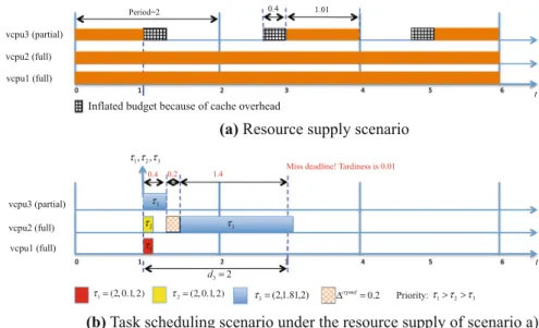
Example 7 Consider a system with a single componentC that has a workloadτ =

{τ1 = τ2 = (2,0.1,2), τ3 = (2,1.81,2)}, which is scheduled under g E D F. We assume that ties are broken based on increasing order of tasks’ indices, i.e., a task with a smaller index has a higher priority. Suppose the cache overhead for each task is given bycrpmd_τ1 =

crpmd

τ2 =0.05 and

crpmd

τ3 =0.2. (The time unit is ms.) In

this example, we consider only the cache overhead caused by VCPU-preemption and VCPU-completion events and assume that there are no other types of overhead.