Generating Timed Trajectories for Autonomous
Robotic Platforms: A Non-Linear Dynamical
Systems Approach
Cristina Manuela Peixoto dos Santos1. Introduction
Over the last years, there have been considerable efforts to enable robots to perform autonomous tasks in the unpredictable environments that characterize many potential applications. An autonomous system must exhibit flexible behaviour that includes multiple qualitatively different types of actions and conforms to multiple constraints. Classically, task planning, path planning and trajectory control are addressed separately in autonomous robots. This separation between planning and control implies that space and time constraints on robot motion must be known before hand with the high degree of precision typically required for non-autonomous robot operation, making it very difficult to work in unknown or natural environments. Moreover, such systems remain inflexible, cannot correct plans online, and thus fail both in non-static environments such as those in which robots interact with humans, and in dynamic tasks or time-varying environments which are not highly controlled and may change overtime, such as those involving interception, impact or compliance. The overall result is a robot system with lack of responsiveness and limited real-time capabilities. A reasonable requirement is that robust behaviour must be generated in face of uncertain sensors, a dynamically changing environment, where there is a continuous online coupling to sensory information. This requirement is especially important with the advent of humanoid robots, which consist of bodies with a high number of degrees-of-freedom (DOFs1).
Behavior-based approaches to autonomous robotics were developed to produce timely robotic responses in dynamic and non-engineered worlds in which linkage between perception and action is attempted at low levels of sensory information (Arkin, 1998). In (Khatib, 1986), some of this planning is made “on-line” in face of the varying sensorial information.
Most current demonstrations of behavior-based robotics do not address timing: The time when a particular action is initiated and terminated is not a controlled variable, and is not stabilized against perturbations. When a vehicle, for instance, takes longer to arrive at a goal because it needed to circumnavigate an obstacle, this change of timing is not compensated for by accelerating the vehicle along its path. Timed actions, by contrast, involve stable temporal relationships. Stable timing is important when particular events must be achieved in time-varying environments such as hitting or catching moving
Access
Database
objects, avoiding moving obstacles, or coordinating multiple robots. Moreover, timing is critical in tasks involving sequentially structured actions, in which subsequent actions must be initiated only once previous actions have terminated or reached a particular phase.
This chapter addresses the problem of generating timed trajectories and sequences of movements for robotic manipulators and autonomous vehicles when relatively low-level, noisy sensorial information is used to initiate and steer action. The developed architectures are fully formulated in terms of nonlinear dynamical systems which lead to a flexible timed behaviour stably adapted to changing online sensory information. The generated trajectories have controlled and stable timing (limit cycle type solutions). Incoupling of sensory information enables sensor driven initiation and termination of movement.
Specifically, we address each of the following questions: (a) Is this approach sufficiently versatile such that a whole variety of richer forms of behaviour, including both rhythmic and discrete tasks, can be generated through limit cycle attractors? (b) Can the generated timed trajectories be compatible with the requirement of online coupling to noisy sensorial information? (c) Is it possible to flexibly generate timed trajectories comprising sequence generation and stably and robust implement them both in robot arms and in vehicles with modest computational resources? Flexibility means here that if the sensorial context changes such that the previously generated sequence is no longer appropriated a new sequence of behaviours, adequate to the current situation, emerges. (d) Can the temporal coordination between different end-effectors be applied to the robotics domain such that a tendency to synchronize among two robot arms is achieved? Can the dynamical systems approach provide a theoretically based way of tuning the movement parameters? (e) Can the proposed timing architecture be integrated with other dynamical architectures which do not explicitly parameterize timing requirements?
These questions are answered in positive and shown in a wide variety of experiments. We illustrate two situations in exemplary simulations. In one, a simple robot arm intercepts a moving object and returns to a reference position thereafter. A second simulation illustrates two PUMA arms perform straight line motion in the 3D Cartesian space such that temporal coordination of the two arms is achieved. As an implementation of the approach, the capacity of a low level vehicle to navigate in a non-structured environment while being capable of reaching a target in an approximately constant time is chosen. The evaluation results illustrate the stability and flexibility properties of the timing architecture as well as the robustness of the decision-making mechanism implemented.
This chapter will give a review of the state of the art of modelling control systems with nonlinear dynamic systems, with a focus on arm and mobile robots. Comments on the relationship between this work, similar approaches and more traditional control methods will be presented and the contributions of this chapter are highlighted. It will provide an overview of the theoretical concepts required to extend the use of nonlinear dynamical systems to temporally discrete movements and discuss theoretical as well as practical advantages and limitations.
2. Background and Related Work
The state of the art described in this chapter addresses the work of the most relevant peers developing research in biologically motivated approaches for achieving movement generation and also addresses a reasonable number of demonstrations in the robotic domain which use dynamic systems for movement generation.
In this chapter, we describe a dynamical system architecture to autonomously generate timed trajectories and sequences of movements as attractor solutions of dynamic systems. The proposed approach is inspired by analogies with nervous systems, in particular, by the way rhythmic and discrete movement patterns are generated in vertebrate animals (Beer et al., 1990; Clark et al., 2000). The vertebrate motor system has only little changed during evolution despite the large variety of different morphologies and types of locomotion. These regularities or invariants seem to indicate some fundamental organizational principles in the central nervous systems (Schaal, 2000). For instance, the basic movements of animals, such as walking, swimming, breathing, and feeding consist of reproducible and representative movements of several physical parts of the body which are influenced by the rhythmic pattern produced in the nervous system. Further, in the presence of a variable environment, animals show adaptive behaviours which require coordination of the rhythms of all physical parts involved, which is important to achieve smooth locomotion. Thus, the environmental changes adjust the dynamics of locomotion pattern generation.
The timing of rhythmic activities in nervous systems is typically based on the autonomous generation of rhythms in specialized neural networks located in the spinal cord, called “central pattern generators” (CPGs). Electrical stimulation of the brain stem of decerebrated animals have shown that CPGs require only very simple signals in order to induce locomotion and even changes of gait patterns (Shik and Orlosky, 1966). The dynamic approach offers concepts with which this timing problem can be addressed. It provides the theoretical concepts to integrate in a single model a theory of movement initiation, of trajectory generation over time and also provides for their control. These ideas have been formulated and tested as models of biological motor control in (Schoner, 1994) by mathematically describing CPGs as nonlinear dynamical systems with stable limit cycle (periodic) solutions. Coordination among limbs can be modelled through mutual coupling of such nonlinear oscillators (Schoner & Kelso, 1988). Coupling oscillators to generate multiple phase-locked oscillation patterns has since long time being used to mathematically model animal behaviour in locomotion (Collins, Richmond, 1994), and to formulate mathematical models of adaptation to periodic perturbation in quadruped locomotion (Ito et al, 1998). This framework is also ideal to achieve locomotion by creating systems that autonomously bifurcate to the different types of gait patterns.
The on-line linkage to sensory information can be understood through the coupling of these oscillators to time-varying sensory information (Schoner, 1994). Limited attempts to extend these theoretical ideas to temporally discrete movements (e.g., reaching) have been made (Schoner, 1990). In this chapter, these ideas are further extended to the autonomous generation of discrete movement patterns (Santos, 2003).
This timing problem is also addressable at the robotics domain. While time schedules can be developed within classical approaches (e.g., through configuration-time space representations), timing is more difficult to control when it must be compatible with continuous on-line coupling to low level and often noisy sensory information which is used to initiate and steer action. One type of solution is to generate time structure at the level of control.
In the Dynamical Systems approach to autonomous robotics (Schoner & Dose, 1992; Steinhage & Schoner, 1998, Large et al, 1999, Bicho et al, 2000), plans are generated from stable states of nonlinear dynamical systems, into which sensory information is fed. Intelligent choice of planning variables makes it possible to obtain complex trajectories and action sequences from stationary stable states, which shift and may even go through
instabilities as sensory information changes. Herein, an extension of this approach is presented to the timing of motor acts, and an attractor based two-layer dynamics is proposed that autonomously generates timed movement and sequences (Schoner & Santos, 2001). This work is further extended to achieve temporal coordination among two DOFs as described in (Santos, 2003). This coordination is achieved by coupling the dynamics of each DOF.
The idea of using dynamic systems for movement generation is not new and recent work in the dynamic systems approach in psychology has emphasized the usefulness of autonomous nonlinear differential equations to describe movement behaviour. In (Raibert, 1986), for instance, rhythmic action is generated by inserting into dynamic control model terms that stabilized oscillatory solutions. Similarly, (Schaal & Atkeson, 1993) generated rhythmic movements in a robot arm that supported juggling of a ball by inserting into the control system a model of the bouncing ball together with terms that stabilized stable limit cycles. Earlier, (Buhler et al., 1994) obtained juggling in a simple manipulator by inserting into the control laws terms that endowed the complete system with a limit cycle attractor. (Clark et al., 2000) describes a nonlinear oscillator scheme to control autonomous mobile robots which coordinates a sequence of basic behaviours in the robot to produce the higher behaviour of foraging for light. (Williamson, 1998) exploits the properties of a simple oscillator circuit to obtain robust rhythmic robot motion control in a wide variety of tasks. More generally, the nonlinear control approach to locomotion pioneered by (Raibert, 1986) amounts to using limit cycle attractors that emerge from the coupling of a nonlinear dynamical control system with the physical environment of the robot. A limitation of such approaches is that they essentially generate a single motor act in rhythmic fashion, and remain limited with respect to the integration of multiple constraints, and planning was not performed in the fuller sense. The flexible activation of different motor acts in response to user demands or sensed environmental conditions is more difficult to achieve from the control level. However, (Schaal & Sternad, 2000) has been able to generate temporally discrete movement as well.
However, there are very few implementations of oscillators for arm and vehicles control. The work presented in this chapter extends the use of oscillators to tasks both on an arm and on a wheeled vehicle. It also differs from most of the literature in that it is implemented on a real robot.
In the field of robotics, the proposed approach holds the potential to become a much more powerful strategy for generating complex movement behavior for systems with several DOFs than classical approaches. The inherent autonomy of the applied approach helps to synchronize systems and thus reduces the computational requirements for generating coordinated movement. This type of control scheme has a great potential for generating robust locomotion and movement controllers for robots. The work proposed is novel because it significantly facilitates movement generation and sequences of movements. Finally, the approach shows up several appealing properties, such as perception-action coupling and reusability of the primitives. The technical motivation is that this framework finds a great number of applications in service tasks (e.g. replacement of humans in industrial tasks and unsafe areas, collaborative work with a human/robot operator) and will permit to advance towards better rehabilitation of movement in amputees (e.g. intelligent and more human like prostheses). In summary, it is expected that in the long run one can potentially increase the application of autonomous robots in tasks for helping the common citizen.
3. The Dynamical Systems Trajectory Generator
In this section, we develop an approach to generate rhythmic and discrete movements. This work is innovative in the manner how it formalizes and uses movement primitives, both in the context of biological and robotics research. We apply autonomous differential equations to model the manner how behaviours related to locomotion are programmed in the oscillatory feedback systems of “central pattern generators” in the nervous systems (Schoner, 1994).
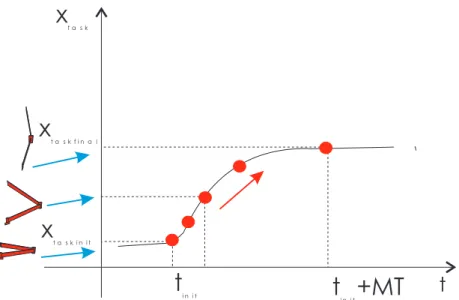
The desired movement is to start at time tinit in an initial postural state2, xtaskinit, and move
to a new final postural state, xtaskfinal, within a desired movement time and keeping that
time stable under variable conditions. Such behavior is what we consider timed discrete movement. Figure 1 illustrates such movement along the X-axis: At time tinit, the system
begins its timed movement between xtaskinit, and xtaskfinal. After a certain movement time,
denominated MT, the movement stops and the system remains at the xtaskfinal position.
In order to understand the concept of discrete movement, consider a two dof robot arm moving in a plane from an initial rest position to a final folded one. The mapping between the robot’s movement and the discrete movement is accomplished through simple coordinate transformations in which the value of the timing variable x is updated.
The initial postural state of discrete movement is mapped onto the initial rest position of the arm. The x oscillatory movement during movement time, MT, corresponds to the arm moving from the initial rest position to the folded one. The final postural position of the discrete movement corresponds to the arm in its final folded position (see Figure 1).
We use the dynamic systems approach to model the desired behaviour, discrete movement, as a time course of the behavioural variables. These variables are generated by dynamical systems.
Figure 1. A discrete movement along the ˆX –axis (as indicated by the black arrow). Mapping of the timing variable x onto the movement of a two dof robot arm
The state of the movement is represented by a single variable, x, which is not directly related to the spatial position of the corresponding effector, but rather represents the effector temporal position within the discrete movement cycle. This temporal position x is then converted by simple coordinate transformations into the correspondent spatial position (Figure 1). Generating oscillatory solutions requires at least two dynamical dof.
Thus, although only the variable x will be used to control motion of a relevant robotic task variable, a second auxiliary variable, y, is needed to enable the system to undergo periodic motion. We could have select
x
$
(2nd order), but instead we select y which provides simplicity to equations that can be easily solved analytically.The entire discrete trajectory is sub-divided into three different behaviours or task constraints: an initial postural state, a stable periodic movement and a final postural state. The implied instability in the switch between these states does not allow to use local bifurcation theory and is difficult to build a general dynamical model which generates this movement as a stable solution (Schoner,1990). The adopted solution is to expresse each constraint as behavioural information (Schoner & Dose, 1992) captured as individual contributions to the dynamical system. Therefore, the trajectories are generated as stable solutions of the following dynamical system, which consists on the combined addition of the contributions of the individual task constraints,
gwn f u f u f u y x final final hopf hopf init init + + + = ⎟⎟⎠ ⎞ ⎜⎜⎝ ⎛ $ $ (1) that can operate in three dynamic regimes controlled by the three “neurons” ui (i = init;
hopf; final). These “neurons” can go “on” (= 1) or “off” (=0), and are also governed by dynamical systems, described later on. The finit and ffinal contributions are described by
dynamical systems whose solutions are stable fixed point attractors (postural states), and the fhopf contribution generates a limit cycle attractor solution. The timing dynamics are
augmented by a Gaussian white noise term, gwn, that guarantees escape from unstable states and assures robustness to the system.
Postural contributions are modelled as attractors of the behavioral dynamics
⎟⎟⎠ ⎞ ⎜⎜⎝ ⎛ − − = ⎟⎟⎠ ⎞ ⎜⎜⎝ ⎛ i post i post y x x y x α $ $ (2) where xi is the current x position of the i movement, xpost is the x postural position and yi is
the y postural position of the i movement (set to zero since it is an auxiliary variable required to enable the system to undergo a periodic motion). These states are characterized by a time scale of
=
1
=
0
.
2
.
post post
α
τ
The Hopf contribution generates the limit cycle solution: the periodic stable movement. We use a well-known mathematical expression, a normal form of the Hopf bifurcation (Perko, 1991), to model the oscillatory movement between two x values:
⎟⎟⎠ ⎞ ⎜⎜⎝ ⎛ + − ⎟⎟⎠ ⎞ ⎜⎜⎝ ⎛ ⎟⎟⎠ ⎞ ⎜⎜⎝ ⎛ − = ⎟⎟⎠ ⎞ ⎜⎜⎝ ⎛ y x y x y x y x h h ) ( 2 2 γ α ω ω α $ $
This simple polynomial equation contains a bifurcation from a fixed point to a limit cycle. We use it because it can be completely solved analytically, providing complete control over its stable states. The limit cycle solution is a periodic oscillation with cycle time
ω
π
2
=
T
and finite amplitude,λ
α
h
A
=
2
. Relaxation to this stable solution occurs at a time scale of: τosc =h
α
2
1
. Further details regarding the Hopf normal form can be found in (Perko, 1991).
An advantage of our specific formulation is the fact that our system is analytically treatable to a large extent, which facilitates the specification of parameters such as
movement time, movement extent, or maximal velocity. This analytical specification is also an innovative aspect of our work.
1.1 Neural Dynamics
The “neuronal” dynamics ui (i = init; final; hopf) switches the timing dynamics from the
fixed point regimes into the oscillatory regime and back. Thus, a single discrete movement act is generated by starting out with neuron |uinit| = 1 activated, the other neurons
deactivated (|uhopf| = |ufinal| = 0), so that the system is in a postural state. The oscillatory
solution is then stabilized (|uinit| = 0; |uhopf | = 1). This oscillatory solution is deactivated
again when the effector reaches its target state, after approximately a half-cycle of the oscillation, turning on the final postural state instead (|uhopf | = 0; |ufinal| = 1). These
various switches are generated by the following competitive dynamics:
(
u u)
u gwn vu u
uinit =µinit init −µinit init3 − 2final + hopf2 init +
α$ (3)
(
u u)
u gwn vu u
uhopf = hopf hopf − hopf hopf − init + init hopf +
2 2 3 µ µ α$ (4)
(
u u)
u gwn v u uufinal = final final − final final − init + hopf final +
2 2 3 µ µ α$ (5)
The first two terms of each equation represent the normal form of a degenerate pitchfork bifurcation. A single attractor at ufp = 0 for negative µi becomes unstable for positive µi, and
two new attractors appear at ufp = 1 and ufp = -1. We use the absolute value of ui as a
weight factor in the timing dynamics, so that +1 and -1 are equivalent “on” states of a neuron, while u = 0 is the “off” state.
The third term in each equation is a competitive term, which destabilizes any attractors in which more than one neuron is “on”. The “neurons”, ui, are coupled through the
parameter υ, named competitive interaction. For positive µi, all attractors of this competitive
dynamics have one neuron in an “on” state, and the other two neurons in the “off” state. In the competitive case, the parameter µi determines the competitive advantage of the
correspondent behavioral variable. That is, among the ui variables, the one with the largest
µi wins (ui = 1) and is turned on, while the others competing variables are turned off (ui =
0). However, for sufficiently small differences between the different µi values multiple
outcomes are possible (the system is multistable)( Large et al., 1999).
1.2 Sequential Activation Criteria
We design functional forms for parameters µi and υ such that the competitive dynamics
appropriately bifurcates to the different types of behaviour in any given situation. These bifurcations happen for certain values of parameters µi and υ, which are in turn dependent
on the environmental situation itself. As the environmental situation changes, the neuronal parameters reflect by design these changes causing bifurcations in the competitive level. To control switching, the parameters, µi (competitive advantages) are
therefore defined as functions of user commands, sensory events, or internal states (Steinhage & Schoner, 1998). Here, we make sure that one neuron is always “on” by varying the µi -parameters between the values 1.5 and 3.5, µi = 1.5 + 2bi,where bi are
“quasi-boolean” factors taking on values between 0 and 1 (with a tendency to have values either close to 0 or close to 1). These “quasi-booleans” express logical or sensory conditions controlling the sequential activation of the different neurons (see (Steinhage & Schoner, 1998; Santos, 2003), for a general framework for sequence generation based on these ideas):
1. binit may be controlled by user input: the command “move” sets binit from the default
value 1 to 0 to destabilize the initial posture. In a first instance binit is controlled by an
initial time set by the user. Thus, its value changes from 1 to 0 when time exceeds tinit:
(
t t)
tbinit( )=σ init − (6)
Herein, σ(.) is a sigmoid function that ranges from 0 for negative argument to 1 for positive argument, selected as
[
tanh(10 ) 1]
/2)
(x = x +
σ (7)
although any other functional form will work as well.
binit may also be controlled by sensory input, such that, for instance, binit changes from 1 to
0 when a particular sensory event is detected. Below we demonstrate how the time-to-contact of an approaching object computed from sensory information can be used to initiate movement in this manner.
2. bhopf is set from 0 to 1 under the same conditions. This term is multiplied, however, with
a second factor bhas not reached target(x) = σ(xcrit - x) that resets bhopf to zero when the effector has
reached its final state. The factor, bhas not reached target(x) has values close to one while the
timing variable x is below xcrit = 0.7 and switches to values close to zero when x comes
within 0.3 of the target state (x = 1). Multiplying two quasi-booleans means connecting the corresponding logical conditions with an “and” operation. Thus, as soon as the timing variable has come within the vicinity of the final state, it autonomously turns the oscillatory state off. In actual implementation, this switch can be driven from the sensed actual position of an effector rather than from the timing dynamics. The final expression for bhopf is:
(
t
t
)
b
arg(
x
)
b
hopf=
σ
−
init hasnotreachedt et (8)3. bfinal is, conversely, set from 0 to 1 when the timing variable comes into the vicinity of
the target: bfinal = 1 - bhas not reached target.
The time scale of the neuronal dynamics is given by τu =
υ
µ
−
−
1
and is set to a relaxation time of τu=0.02, ten times faster than the relaxation time of the timing variables. This
difference in time scale guarantee that the analysis of the attractor structure of the neural dynamics is unaffected by the dependence of its parameters, µi on the timing variable, x,
which is a dynamical variable as well. Strictly speaking, the neural and timing dynamics are thus mutually coupled. The difference in time scale makes it possible to treat x as a parameter in the neural dynamics (adiabatic variables). Conversely, the neural weights can be assumed to have relaxed to their corresponding fixed points when analyzing the timing dynamics (adiabatic elimination). The adiabatic elimination of fast behavioral variables reduces the complexity of a complicated behavioural system built up by coupling many dynamical systems (Steinhage & Schöner, 1998; Santos, 2003). By using different time scales one can design the several dynamical systems separately.
1.3 An Example: A Timed Temporally Discrete Movement Act
Periodic movement can be trivially generated from the timing and neural dynamics by selecting uhopf “on” through the corresponding quasi-booleans. A timed, but temporally
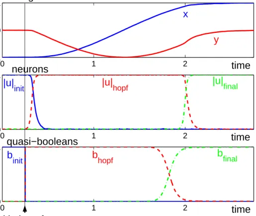
discrete movement act, is autonomously generated by these two coupled levels of nonlinear dynamics through a sequence of neural switches, such that an oscillatory state exists during an appropriate time interval of about a half-cycle. This is illustrated in Figure
2. The timing variable, x, which is used to generate effector movement, is initially in a postural state at -1, the corresponding neuron uinit being “on”. When the user initiates
movement, the quasi-booleans, binit and bhopf exchange values, which leads, after a short
delay, to the activation of the “hopf” neuron. This switch initiates movement, with x evolving along a harmonic trajectory, until it approaches the final state at +1. At that point, the quasi-boolean bfinal goes to one, while bhopf changes to zero. The neurons switch
accordingly, activating the final postural state, so that x relaxes to its terminal level x = 1. The movement time is approximately a half cycle time, here MT = 2.
2. Simulation of a Two Dof Arm Intercepting a Ball
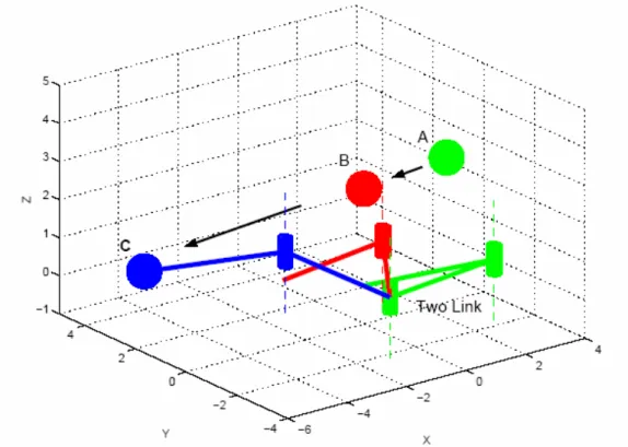
As a toy example of how the dynamical systems approach to timing can be put to use to solve robotic problems, consider a two dof robot arm moving in a plane (Figure 3).
The task is to generate a timed movement from an initial posture to intercept an approaching ball. Movement with a fixed movement time (reflecting manipulator constraints) must be initiated in time to reach the ball before it arrives in the plane in which the arm moves. Factors such as reachability and approach path of the ball are
0 1 2 −1 0 1 0 1 2 0 1 0 1 2 0 1
quasi−booleans
neurons
timing variables
initiation of movement
|u|
hopf
|u|
finalb
finalb
initb
hopfx
y
time
time
time
|u|
initFigure 2. Simulation of a user initiated temporally discrete movement represented by the timing variable, x, which is plotted together with the auxiliary variable, y, in the top panel. The time courses of the three neural activation variables, uinit, uhopf, and ufinal, which control the timing dynamics, are shown in the middle panel.
The quasi-boolean parameters, binit, bhopf, and bfinal, plotted on bottom, determine the competitive advantage of
each neuron
continuously monitored, leading to a return of the arm to the resting position when interception becomes impossible (e.g., because the ball hits outside the workspace of the arm, the ball is no longer visible, or ball contact is no longer expected within a criterion time-to-contact). After the ball interception, the arm moves back to its resting position, ready to initiate a new movement whenever appropriate sensory information arrives.
In order to formulate this task using the nonlinear dynamical systems approach, three relevant coordinate systems are defined: a) The timing variable coordinate system, {P}3,
describes the timing variable position along a straight path from the initial to the final postural position. This is a conceptual frame, in which temporal movement is planned. b) The task reference coordinate system (universal coordinate system) describes the end-effector position, (x, y, z), of the arm along a straight path from the initial position (initial posture) to the target position (computed coordinates of point of interceptance) and the ball position. c) The base coordinate system {R} is attached to the robot's base and the arm kinematics is described by two joint angles in this frame.
Figure 3. A two dof arm intercepts an approaching ball. Corresponding ball and arm positions are illustrated by using the same grey-scale. The first position (light grey) is close to the critical time-to-contact, where arm motion starts. The last position (dark grey) is close to actual contact. The black arrows indicate the ball's movement
The timing variable coordinate system {P} is positioned such that Px coordinates vary
between -1 and +1, with Py and Pz coordinates equal to zero. Px is scaled to the desired
amplitude, A, dependent on the predicted point of interceptance.
Frame (a) and (b) are linked through straightforward formulae, which depend on the predicted point of interceptance, (x(τt2c); y(τt2c);) in the task reference frame. Frame (b) and
(c) are linked through the kinematic model of the robot arm and its inverse (which is exact).
During movement execution, the timing variables are continuously transformed into task frame (b), from which joint angles are computed through the inverse kinematic transformation. The solutions of the applied autonomous differential equations are converted by simple coordinate transformations, using model-based control theory, into motor commands.
3
However, in the text, the timing variables P
x and P
y are referred to as timing variable x, y without
2.1 Coupling to Sensorial Information
In order to intercept an approaching ball it is necessary to be at the right location at the right time. We use the visual stimulus as the perception channel to our system. In these simulations we have extracted from a simulated ball trajectory two measures: the time-to-contact, τt2c, and the point-of-contact. The robot arm intersects the ball on the plane of the
camera (mounted on its base) such that the ball's movement crosses the observer (or image) plane (zB = 0). The time it takes to the ball to intersect the arm at this point in space,
that is, the time-to-contact, is extracted from segmented visual information without having estimated the full cartesian trajectory of the ball (Lee, 1976). We consider the ball has a linear trajectory in the 3D cartesian space with a constant approach constant velocity. The point of contact can be computed along similar lines if the ball size is assumed to be known and can be measured in the image.
To simulate sensor noise (which can be substantial if such optical measures are extracted from image sequences), we added either white or coloured noise to the estimated time-to-contact. Here we show simulations that used coloured noise, ξ, generated from
gwn Q corr + − = τ ζ ζ 1 (9)
where gwn is gaussian white noise with zero mean and unit variance, so that Q = 5 is the effective variance.
The correlation time, τcorr, was chosen as 0.2 sec. The simulated time-to-contact was thus
) (
2c true time to contact t
t ζ
τ = − − + (10)
2.2 Behavior Specifications
These two measures, time-to-contact and point-of-contact, fully control the neural dynamics through the quasi-boolean parameters. A sequence of neural switches is generated by translating sensory conditions and logical constraints into values for these parameters. For instance, the parameter, binit, controlling the competitive advantage of the
initial postural state must be “on” (= 1) when the timing variable x is close to the initial state -1, and either of the following is true: a) Ball not approaching or not visible (τt2c≤ 0).
b) Ball contact not yet within a criterion time-to-contact (τt2c > τcrit). c) Ball is approaching
within criterion time-to-contact but is not reachable (0 <τt2c < τcrit; breachable = 0).
These logical conditions can be expressed through this mathematical function:
binit =σ(−xcrit−x)
[
σ(τt2c−τcrit)+σ(τt2c)σ(τcrit−τt2c)σ(1−breacchable)+σ(−τt2c)]
(11) where σ(.) is the threshold-function used earlier (Equation 7).The “or” is realized by summing terms which are never simultaneously different from zero. In other cases, the “or” is expressed with the help of the “not” (subtracting from 1) and the “and”. This is used in the following expressions for bhopf and bfinal which can be
derived from a similar analysis:
[
]
{
}
[
( ) (1 ) ( ) ( ) ( )]
) 1 ( ) ) ( ) ( ) ( ) ( 1 ( 1 2 2 2 2 x x b x x b x x b crit crit c t c t reacchable crit reacchable c t crit c t crit hopf − + − + − + − + − − − − − = σ τ τ σ τ σ σ σ σ τ τ σ τ σ σ (12) ) ( ) ( ) ( )( t2c crit t2c reacchable crit
final b x x
b =σ τ σ τ −τ σ +σ − (13)
2.3 Properties of the Generated Timed Trajectory
approaches, the current time-to-contact becomes smaller than a critical value (here 3), at which time the quasi-boolean for motion, bhopf becomes one, triggering activation of the
corresponding neuron, uhopf, and movement initiation. Movement is completed (x reaches
the final state of +1) well before actual ball contact is made. The arm waits in the target posture. In this simulation the ball is reflected upon contact. The negative time-to-contact observed then leads to autonomous initiation of the backward movement to the arm resting position.
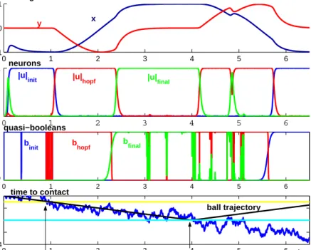
The fact that timed movement is generated from attractor solutions of a nonlinear dynamical system leads to a number of properties of this system, that are potentially useful to real-world implementations of this form of autonomy. The simulation shown in Figure 4 illustrates how the generation of the timing sequence resists against sensor noise: the noisy time-to-contact data led to strongly fluctuating quasi-booleans (noise being amplified by the threshold functions). The neural and timing dynamics, by contrast, are not strongly affected by sensor noise so that the timing sequence is performed as required. When simulations with this level of sensor noise are repeated, failure is never observed, although there are instances of missing the ball at even larger noise levels. By simulating strong sensor noise we demonstrate that the approach is robust. Note how the autonomous sensor-driven initiation of movement is stabilized by the hysteresis properties of the competitive neural dynamics, so that small fluctuations of the input signal back above threshold do not stop the movement once it has been initiated (Schoner & Dose, 1992; Schoner & Santos, 2001).
The design of the quasi-boolean parameters of the competitive dynamics guarantees that flexibility is fulfilled: if the sensorial context changes such that the previously generated sequence is no longer adequate, the plan is changed and a new sequence of events emerges. 0 1 2 3 4 5 6 −1 0 1 0 1 2 3 4 5 6 0 1 2 3 4 5 6 0 1 2 3 4 5 6 −4 0 4 y x |u| final |u|
init |u|hopf
b hopf b init bfinal time to contact time to contact reaches threshold ball contact and reflection ball trajectory time quasi−booleans neurons timing variables 0 1 1 0
Figure 4. Trajectories of variables and parameters in autonomous ball interception and return to resting position. The top three panels represent timing variables, neural variables and quasi-booleans. The bottom panel shows the time-to-contact, which crosses a threshold at about 0:5 time units. When contact is made, the ball is assumed to be reflected, leading to negative time-to-contact
When sensory conditions change an appropriate new sequence of events emerges. When one of the sensory conditions for ball interception is invalid (e.g., ball becomes invisible, unreachable, or no longer approaches with appropriate time-to-contact), then one of the following happens depending on the point within the sequence of events at which the change occurs: 1) If the change occurs during the initial postural stage, the system stays in that postural state. 2) If the change occurs during the movement, then the system continues on its trajectory, now going around a full cycle to return to the reference posture. 3) When the change occurs during posture in the target position, a discrete movement is initiated that takes the arm back to its resting position.
The decision is dependent on local information available at the system's current position: on the current location of the timing variable, x, on the time-to-contact and point-of-contact information currently available. The non-local sequence of events is generated through local information without needing symbolic representations of the behaviours. This is achieved by obeying the principles of the Dynamic Approach and illustrates the power of our approach: the behaviour of the system itself leads to the changing sensor information which controls the change and persistence of a rich set of behaviors.
Consider the ball is suddenly shifted away from the arm at about 1.9 time units, leading to much larger time-to-contact, well beyond threshold for movement initiation. In Figure 5, time-to-contact becomes suddenly larger than the critical value when the arm is in its motion stage: uhopf neuron is activated and the other neurons are deactivated. The uhopf
neuron rests activate while the arm continues its movement a full cycle. At the time the x timing variable is captured by the initial postural state (x = -1), the quasi-boolean binit
becomes one, triggering the activation of the neuron, uinit, and bhopf becomes zero,
deactivating the corresponding neuron uhopf. The arm rests in the reference position. This
behaviour emerges from the sensory conditions controlling the neuronal dynamics.
0 1 2 3 4 5 6 −1 0 1 0 1 2 3 4 5 6 0 0.5 1 0 1 2 3 4 5 6 0 1 2 3 4 5 6 −4 0 5 x y timing variables u init uhopf u final neurons quasi−booleans time to contact time time to contact reaches threshold
ball is perturbed increasing time to contact beyond threshold
0 1
b
init bhopf
bfinal
Figure 5. Similar to Figure 4, but the ball is suddenly shifted at about 1.9 time units leading to a time to contact larger than the threshold value (3) required for movement initiation
3. Coupling among Two Timing Systems
Another task illustrating uses of the dynamical systems approach to timing is the temporal coordination of different dofs. In robotics, the control of two dof is generally achieved by considering the dofs are completely independent. Therefore, this problem reduces to the one of controlling two robot arms instead of one. However, in motor control of biological systems where there are numerous dofs, this independence is not verified. Movement coordination requires some form of planning: every dof needs to be supplied with appropriate motor commands at every moment in time. However, there exist actually an infinite number of possible movement plans for any given task. A rich area of research has been evolving to study the computational principles and implicit constraints in the coordination of multiple dofs, specifically the question whether or not there are specific principles in the organization of central nervous systems, that coordinate the movements of individual dofs. This research has been mainly directed towards coordination of rhythmic movement. In rhythmic movements, behavioural characteristics show off in that the oscillations verified in these dofs remain coupled in-phase, and also because the dofs show a tendency to become coupled in a determined way (Schaal, 2000). In reaching movements, behavioural characteristics reveal in the synchronization and/or sequencing of movements with different on-set times.
The coordination of rhythmic movements has been addressed within the dynamic theoretical approach (Schoner,1990). These dynamic concepts can be generalized to understand the coordination of discrete movement. Temporal coordination of discrete movements is enabled through the coupling among the dynamics of several such systems such that in the periodic regime the two forms of movement, stable in-phase and anti-phase, are recovered. This is achieved by introducing a discrete movement for each dof (end-effector), and two dofs are considered. The idea is to couple the two discrete movements with the same frequency in a specific way, determined by well established parameters, such that within a certain time the two movements become locked at a given relative phase. The coupling term is multiplied with the neuronal activation of the other system's “Hopf” state such that coupling is effective only when both components are in movement state. This is achieved by modifying the "Hopf" contribution to the timing dynamics as follows ... ) ( ) , ( ... 1 2 1 2 2 , 1 1 1 , 1 , 1 1 ⎥ ⎦ ⎤ ⎢ ⎣ ⎡ ⎟⎟⎠ ⎞ ⎜⎜⎝ ⎛ − − + + = ⎟⎟⎠ ⎞ ⎜⎜⎝ ⎛ y y x x cR u y x f u y x hopf hopf hopf θ $ $ (14) ... ) ( ) , ( ... 2 1 2 1 1 , 2 2 2 , 2 , 2 2 ⎥ ⎦ ⎤ ⎢ ⎣ ⎡ ⎟⎟⎠ ⎞ ⎜⎜⎝ ⎛ − − − + + = ⎟⎟⎠ ⎞ ⎜⎜⎝ ⎛ y y x x cR u y x f u y x hopf hopf hopf θ $ $ (15) where index i = 1, 2 refers to the dof 1 and 2, respectively, and θ is the desired relative phase. This coordination through coupling approaches the generation of coordinated patterns of activation in locomotory behaviour of nervous biological systems.
3.1 An Example: Two 6 Dof Arms Coupled
Consider two PUMA arms performing a straight line motion in 3D Cartesian space (Schoner & Santos, 2001; Santos, 2003). In the simulations, the inverse kinematics of the PUMA arms were based on the exact solution. Each robot arm initiates its timed movement from an initial posture to a final one. Movement parameters such as initial posture, movement initiation, amplitude and movement time are set for each arm individually.
Each arm is driven by a complete system of timing and neural dynamics. Further, the two timing dynamics are coupled as described by Equations 14 and 15. The specified relative phase is θ = 0º. In discrete motor acts, a coupling of this form tends to synchronize movement in the two components, a tendency captured in terms of relative timing of the movements of both components. The two robot arms are temporally coordinated: if movement parameters such as movement on-sets or movement times are not identical, the control level coordinates the two components such that the two movements terminate approximately simultaneously.
This coupling among two timing systems helps synchronize systems and reduces the computational requirements for determining identical movement parameters across such components. Even if there is a discrepancy in the MT programmed by the parameter ω of the timing dynamics, coupling generates identical effectives MTs. This discrete analogue of frequency locking is illustrated in left panel of Figure 6.
0 1 2 3 4 −1 0 Time uncoupled coupled x1u x2u x2c x1c 0 1 2 3 4 −1 0 1 Time uncoupled coupled x1c x1u x 2c x 2u
Figure 6. a) Coordination between two timing dynamics through coupling leads to synchronization when movement times differ (2 vs. 3). b) Movement initiation is slightly asynchronous tinit1 = 1 and tinit2 = 1.4s (∆tinit
= 5 % of MT), MT1 = MT2 = 2s and c = 1)
This tendency to synchronize is also verified when both movements exhibit equal movement times but the on-sets are not perfectly synchronized (right panel of Figure 6). In this case, the effect in the delayed component is to move faster, again in the direction of restoring synchronization.
In case we set a relative phase of θ = 180º we verify anti-phase locking. In the case of discrete movement, anti-phase locking leads to a tendency to perform movements sequentially. Thus, if movement initiation is asynchronous, the movement time of the delayed movement increases such that the movements occur with less temporal overlap.
4. Integration of Different Dynamical Architectures
As an implementation of the approach, the capacity of a low level vehicle to navigate in a non-structured environment while being capable of reaching a target in an approximately constant time is chosen.
4.1 Attractor Dynamics for Heading Direction
The robot action of turning is generated by varying the robot's heading direction, φh,
(Schöner and Dose, 1992). This behavioural variable is governed by a nonlinear vector field in which task constraints contribute independently by modelling desired behaviours (target acquisition) as attractors and undesired behaviours (obstacle avoidance) as repellers of the overall behavioural dynamics (Bicho, 2000).
Target location, (xB, yB), is continuously extracted from visual segmented information
acquired from the camera mounted on the top of the robot and facing in the direction of the driving speed. The angle φh of the target's direction as “seen” from the robot is:
B B x y tar R B R B tar
R
R
x
x
y
y
arctan
arctan
⇔
=
−
−
=
φ
φ
(16)where (xR, yR) is the current robot position in the allocentric coordinate system as given by
the dead-reckoning mechanism.
Integration of the target acquisition (behaviour ftar) and obstacle avoidance (behaviour fobs)
contributions is achieved by adding each of them to the vector field that governs heading direction dynamics
)
(
)
(
)
(
)
(
h stoch h tar h obs hF
f
f
dt
d
φ
φ
φ
φ
=
+
+
(17)We add a stochastic component force, Fstoch, to ensure escape from unstable states within a
limited time. The complete behavioural dynamics for heading direction has been implemented and evaluated in detail on a physical mobile robot (Bicho, 2000).
4.2 The Dynamical Systems of Driving Speed
Robot velocity is controlled such that the vehicle has a fixed time to reach the target. Thus, if the vehicle takes longer to arrive at the target because it needed to circumnavigate an obstacle, this change of timing must be compensated for by accelerating the vehicle along its path.
The path velocity, v, of the vehicle is controlled through a dynamical system architecture that generates timed trajectories for the vehicle. We set two spatially fixed coordinates frames both centred on the initial posture, which is the origin of the allocentric coordinate system: one for the x and the other for the y spatial coordinates of robot movement. A complete system of timing and neural dynamics is defined for each of these fixed coordinate frames. Each model consists of a timing layer (Schoner & Santos, 2001), which generate both stable oscillations (contribution fhopf) and two stationary states
(contributions “init” and “final”).
gwn
f
u
f
u
f
u
a
x
i final i final i hopf i hopf i init i init i i+
+
+
=
⎟⎟⎠
⎞
⎜⎜⎝
⎛
, , , , , ,$
$
(18) where the index i = x, y refers to timing dynamics of x and y spatial coordinates of robot movement. A neural dynamics controls the switching between the three regimes through three neurons, uj,i (j = init, hopf, final) (Equation 20). The “init” and “final” contributionsgenerate stable stationary solutions at xi = 0 for “init” and Aic for “final” with ai = 0 for
both. These states are characterized by a time scale of τ = 1/5 = 0.2. The “Hopf” contribution to the timing dynamics is defined as follows:
⎟
⎟
⎠
⎞
⎜
⎜
⎝
⎛ −
⎟⎟⎠
⎞
⎜⎜⎝
⎛
+
⎟
⎠
⎞
⎜
⎝
⎛ −
−
⎟
⎟
⎠
⎞
⎜
⎜
⎝
⎛ −
⎟⎟⎠
⎞
⎜⎜⎝
⎛
−
=
i ic i i ic i i i ic i h h i hopfa
A
x
a
A
x
a
A
x
f
2
2
2
2 2 ,γ
α
ω
ω
α
(19) where4
2 ic h iA
α
λ
=
defines amplitude of Hopf i contribution.4.3 Behavioural Specifications
The neuronal dynamics of uj,i∈ [-1; 1] (j = init, hopf, final) switches each timing dynamics
from the initial and final postural states into the oscillatory regime and back, and are given by
gwn
u
u
v
u
u
u
j a i j i a i j i j i j i j i j u=
−
−
∑
+
≠ , 2 , 3 , , , , ,µ
µ
α
$
(20)We assure that one neuron is always “on” by varying the µi -parameters between the
values 1.5 and 3.5: µi = 1.5 + 2bi, where bi are the quasi-boolean factors.
The competitive advantage of the initial postural state is controlled by the parameter binit.
This parameter must be “on” (= 1) when either of the following is true: (1) time, t, is bellow the initial time, tinit, set by the user (t < tinit); (2) timing variable xi is close to the initial state
0 (bxi close xinit (xi)); and time exceeds tinit (t > tinit); and target has not been reached.
We consider that the target has not been reached when the distance, dtar, from the actual
robot position (as internally calculated through dead-reckoning) and the (xtarget, ytarget)
position is higher than a specified value, dmargin. This logical condition is expressed by the
quasi-boolean factor, bxi has not reached target(dtar) = σ(dtar-dmargin), where σ(.) is the sigmoid
function explained before (Equation 7). Note that this switch is driven from the sensed actual position of the robot.
The factor bxi close xinit (xi) = σ( xcrit-xi) has values close to one while the timing variable xi is
bellow 0.15Aic and switches to values close to zero elsewhere.
These logical conditions are expressed through the mathematical function:
(
)
[
(
( )(
)
( )
)
]
}
{
t
t
b
x
t
t
b
d
b
init=
1
−
≥
init1
−
xiclosexinit i≥
init xihasnotreachedtarget (21) A similar analysis derives the bhopf and bfinal parameters:(
init)
xinotclosexfinal( )
i xi hasnotreachedt et( )
tar(
updateAic)
hopf t t b x b d b
b = ≥ arg σ (22)
(
init)
[
xinotclosexfinal( )
i xireachedt et( )
tar xinotclosexfinal( )
i(
(
updateAic)
)
]
final t t b x b d b x b
b = ≥ + arg + + 1−σ (23)
We algorithmically turn off the update of the i timed target location, Txtarget or Tytarget, once
this changes sign relatively to the previous update and the corresponding timing level is in the initial postural state.
The factor bxi not close xfinal (xi) = σ(dswitch - dcrit) is specified based on absolute values, where
dswitch represents the distance between the timing variable xi and the final postural state,
Aic and dcrit is tuned empirically.
The competitive dynamics are the faster dynamics of the all system. Its relaxation time, τu,
is set ten times faster than the relaxation time of the timing variables (τu = 0.02).
The system is designed such that the planning variable is in or near a resulting attractor of the dynamical system most of the time. If we control the driving velocity, v, of the vehicle, the system is able to track the moving attractor. Robot velocity depends whether or not obstacles are detected for the current heading direction value. This velocity depends on
the behaviour exhibited by the robot and is imposed by a dynamics equal to that described by (Bicho et al, 2000)
(
)
(
)
⎟⎟ ⎠ ⎞ ⎜ ⎜ ⎝ ⎛ − − − − ⎟⎟⎠ ⎞ ⎜⎜⎝ ⎛− − − − = 2 2 min min min 2 2 2 ) ( exp 2 ) ( exp v g ti g ti g ti v obs obs obs V v V v c V v V v c dt dv σ σ (24)Vobs is computed as a function of distance and is activated when an obstacle is detected.
Vtiming is specified by the temporal level as
2 2 ming x y
ti x x
V = $ + $ (25)
For further details regarding this dynamics refer to (Bicho, 2000).
The following hierarchy of relaxation rates ensures that the system relaxes to the stable solutions, obstacle avoidance has precedence over target acquisition and target achievement is performed in time tar obs tar g ti v obs v obs v τ τ τ τ τ τ , << , , , min << , << (26)
Suppose that at t = 0 s the robot is resting at an initial fixed position, the same as the origin of the allocentric coordinate system. The robot rotates in the spot in order to orient towards the target direction. At time tinit, the quasi-boolean for motion, bhopf, becomes one,
triggering activation of the corresponding neuron, uhopf, and movement initiation.
Movement initiation is accomplished by setting the driving speed, v, different from zero. During periodic movement, the target location in time is updated each time step based on error, xR - Txx, such that
(
x)
T R et t et t Tx
x
x
x
arg=
arg−
−
(27)where Txx is the current timing variable xx, xr is the x robot position and is the timing
variable xx. The periodic motion's amplitude, Axc, is set as the distance between Txtarget and
the origin of the allocentric reference frame (which is coincident with the x robot position previously to movement initiation), such that
( )
t
x
( )
t
A
t etT
xc
=
arg (28)The periodic solution is deactivated again when the vehicle comes into the vicinity of the x timed target, and the final postural state is turned on instead (neurons |uhopf| = 0; |ufinal|
= 1). At this moment in time, the x timed target location is no longer updated in the timing dynamics level.
The same behaviour applies for the timing level defined for the y spatial coordinate.
4.4 Experimental Results
The dynamic architecture was implemented and evaluated on an autonomous wheeled vehicle (Santos, 2004). The dynamics of heading direction, timing, competitive neural, path velocity and dead-reckoning equations are numerically integrated using the Euler method with fixed time step.
Image processing has been simplified by working in a structured environment, where a red ball lies at coordinates (xB; yB) = (-0.8; 3.2) m (on the allocentric coordinate system) on the top of a table at approximately 0.9m tall. The initial heading direction is 90 degrees. The sensed obstacles do not block vision. An image is acquired only every 10 sensorial cycles such that the cycle time is 70 ms, which yields a movement time (MT4) of 14s. Forward
4
movement initiation is triggered by an initial time set by the user and not from sensed sensorial information. Forward movement only starts for tinit = 3s.
The rotation speeds of both wheels are computed from the angular velocity, w, of the robot and the path velocity, v. The former is obtained from the dynamics of heading direction. The later, as obtained from the velocity dynamics is specified either by obstacle avoidance contribution or the timing dynamics. By simple kinematics, these velocities are translated into the rotation speeds of both wheels and sent to the velocity servos of the two motors.
A. Properties of the Generated Timed Trajectory
The sequence of video images shown in Figure 7 illustrates the robot motion in a very simple scenario: during its path towards the target, the robot faces two obstacles separated of 0.7m, which is a distance larger enough for the robot to pass in between. The time courses of the relevant variables and parameters are shown in Figure 8.
At time t = 7.2 s obstructions are detected and the velocity dynamics are dominated by the obstacle constraints (bottom panel of Figure 8). Due to obstructions circumnavigation, the robot position differs from what it should be according to the timing layer (at time t = 11.5s). The x robot position is advanced relatively to the Tx
x timing dynamics specifications
and Axc is decreased relatively to xtarget (Figure 8).
Figure 7. Robot motion when the robot faces two objects separated of 0.7m during its path. The robot successfully passes through the narrow passage towards the target and comes to rest at a distance of 0.9m near the red ball at t = 16.56s. The effective movement time is 13.56 s
Therefore, the robot velocity is de-accelerated in this coordinate. Conversely, the y robot position lags the Tx
(third panel of Figure 8). Finally, the target is reached and the robot comes to rest at a distance of 0.90m near the red ball. The overall generated timed trajectory takes t = 16.56 - 3 s to reach the target (forward movement started at time t = 3s).
This trajectory displays a number of properties of dynamical decision making. Figure 8 shows how the hysteresis property allows for a special kind of behavioral stability. At t = 15s the quasi-boolean parameter bx,hopf becomes zero but the ux,hopf neuron remains
activated until the neuron ux,final is more stable, what happens around t = 16.2s. At this
time, the x periodic motion is turned off. Thus, hysteresis leads to a simple kind of memory which determines system performance depending on its past history.
Figure 9 shows the robot trajectory as recorded by the dead-reckoning mechanism when the distance between the two obstacles is smaller than the vehicle's size (0.3m). The path followed by the robot is qualitatively different. In case timing dynamics stabilize the velocity dynamics the robot is strongly accelerated in order to compensate for the object circumnavigation. Light crosses on the robot trajectory indicate robot positions where vision was not acquired because the robot could not see the ball. The ball position as calculated by the visual system slight differs from the real robot position (indicated by a dark circle).
B. Trajectories Generated with and without Timing Control
Table 1 surveys the time the robot takes to reach the target lying at coordinates (-0.8, 3.24) m for several configurations when path velocity, v, is controlled with and without timing control. In the latter, path velocity is specified differently: when no obstructions are detected the robot velocity is stabilized by an attractor, which is set proportional to the distance to the target (Bicho, 2000). Note that forward movement starts immediately. Conversely, forward movement only happens at t = 3 s when there is timing control. The specified movement time is 14s.
0 5 10 15 −1 0 0.5 0 5 10 15 0 1 0 5 10 15 0 1 0 5 10 15 0 2 timing variables neurons quasi−booleans time (s) xx Axc yx xtarget ux,hopf ux,final ux,init bx,init bx,hopf bx,final start dtarget dswitch 0 5 10 15 −1 0 2 0 5 10 15 0 1 0 5 10 15 0 1 0 5 10 15 0 2 timing variables neurons quasi−booleans time (s) ytarget Ayc xy yy uy,init uy,hopf uy,final by,init by,hopf by,final dswitch dtarget start 0 5 10 15 −1 0 1 0 5 10 15 −1 0 0 5 10 15 0 1 2 0 5 10 15 0 0.2 uy,hopf ux,hopf U(φ) xR Tx x xtarget Axc Ayc T xy ytarget yR vobs v vtiming time (s)
Figure 8. Time courses of variables and parameters for the robot trajectory depicted in Figure 7. Top panels depict timing and neural dynamics (x and y coordinate in left and right panels, respectively). Bottom panel depicts neural and timing variables, robot trajectories, real target locations, periodic motion amplitudes and velocity variables.
We observe that both controllers have stably reached the target but the former is capable of doing it in an approximately constant time independently of the environment configuration.
Experiments Time to reach target with timing and MT
Time to reach target without timing No obstacles 16.8 (13.8) 18.6 One obstacle 16.6 (13.6) 19.0 obstacles separated 0.8m 16.5 (13.5) 18.9 obstacles separated 0.7m 16.6 (13.6) 19.0 obstacles separated 0.3m 18.8 (15.8) 23.6 Complex configuration 1 19.3 (16.3) 22.5 Complex configuration 2 17.2 (14.2) 19.2 Complex configuration 3 17.4 (14.4) 19.6 Complex configuration 4 16.8 (13.8) 19.7 Complex configuration 5 17.3 (14.3) 18.3 Complex configuration 6 17.7 (14.7) 19.8 Complex configuration 7 23.3 (20.3) 28.0
Table 1. Time (in seconds) the robot takes to reach a target for several environment configurations, when robot’s forward velocity, v, is controlled with and without timing control
We have also compared time the robot takes to reach the target when velocity is controlled with and without timing control for different target locations and same configurations as in Table 1. The results have shown that the achieved movement time is approximately constant and independent of the distance to the target.
−1.0 0 0 1 2 3 4 x y
Figure 9. Robot trajectory as recorded by the dead-reckoning mechanism when obstacles are separated of 0.3m
5. Conclusion and Discussion
This paper addressed the problem of generating timed trajectories and sequences of movements for autonomous vehicles when relatively low-level, noisy sensorial information is used to initiate and steer action. The developed architectures are fully formulated in terms of nonlinear dynamical systems. The model consists of a timing layer
with either stable fixed points or a stable limit cycle. The qualitative dynamics of this layer is controlled by a neural competitive dynamics. By switching between the limit cycle and the fixed points, discrete movements and sequences of movements are obtained. These switches are controlled by the parameters of the neural dynamics which express sensory information and logical conditions. Coupling to sensorial information enables sensor driven and initiation. To corroborate the proposed solution experiments were performed using robot arms and low-level autonomous vehicles. The implemented decision making mechanism allowed the system to flexibly respond to the demands of the sensed environment at any given situation. The generated sequences were stable and a decision maintained stable by the hysteresis property. The described implementation in hardware probes how the inherent stability properties of neural and timing dynamics play out when the sensory information is noisy and unreliable.
Some aspects are unique to this work and have enabled the introduction of timing constraints. We have shown how the attractor dynamics approach to the generation of behaviour can be extended to the timing of motor acts. Further, we have shown that by manipulating the timing of a limit cycle the system performed well tasks with complex timing constraints.
The dynamical systems approach has various desirable properties. Firstly, its inherent properties, such as temporal, scale and translation invariance relatively to the tuning parameters, provide the ability to modify online the generated attractor landscape to the demands of the current situation, depending on the sensorial context. Because movement plans are generated by the time evolution of autonomous differential equations, they are not explicitly indexed by time, and thus by means of coupling perceptual variables to the dynamic equations, they can accomplish flexible on-line modification of the basic behaviors. This property enables to create several forms of on-line modifications, e.g., based on contact forces in locomotion, perceptual variables in juggling or the tracking error of a robotic system (Ijspeert et al., 2002). A globally optimized behaviour is achieved through local sensor control and global task constraints, expressed through the logics contained in the parameters of the differential equations and not in an explicit program. A smooth stable integration of discrete events and continuous processes is thus achieved. Further, we guarantee the stability and the controllability of the overall system by obeying the time scale separation principle. Further, this approach does not make unreasonable assumptions, or place unreasonable constraints on the environment in which the robot operates and assures a quick reaction to eventual changes in the sensed environment. The ease with which the system is integrated into larger architectures for behavioural organization that do not necessarily explicitly represent timing requirements is a specific advantage of our formulation. This integration enables to achieve behavioural organization. By obeying the time scale separation principle we design the ordering principle for the coupled behavioural dynamics. This scalability property implies a high modularity. On the opposite, the integration of new behaviours, using symbolic representations, obliges to redesign the whole behavioural system.
Another advantage of our specific formulation is the fact that it is possible to parameterize the system by analytic approximation, which facilitates the specification of parameters such as movement time, movement extent, maximal velocity, etc. Not only we have generated discrete movement as well as we provide a theoretically based way of tuning the dynamical parameters to fix a specific movement time or extent. Comparatively, other non-linear approaches, such as (Buhler et al, 1994; Raibert, 1986), the overall movement parameters emerge from the interaction of the control system with the environment so that
achieving specific movement times or amplitudes is only possible by empirical tuning of parameters. While these approaches only achieved rhythmic movement, (Schaal et al., 2000) have, like us, been able to generate temporally discrete movement as well. It does not appear, however, that there is a theoretically based way of tuning the dynamical parameters to fix a specific movement time or extent.
Further, the approach is a powerful method for obtaining temporal coordinated behaviour of two robot arms. The coupled dynamics enable synchronization or sequentialization of the different components providing an independency relatively to the specification of their individual movement parameters. Such coupling tends to synchronize movement in the two components such that the computational requirements for determining identical movement parameters across such components are reduced. From the view point of engineering applications, the inherent advantages are huge, since the control system is released from the task of recalculating the movement parameters of the different components.
6. References
Arkin, R C. (1998) Behavior-Based Robotics. MIT Press, Cambridge.
Bajcsy, R. and Large, E. (1999) When and where will AI meet robotics? AI Magazine, 20:57-65.
Beer, R D; Chiel, H J and Sterling, L S. (1990) A biological perspective on autonomous agent design. Robotics and Autonomous Systems, 6:169-189.
Bicho, E. (2000) Dynamic Approach to Behavior-based Roboti