Packet-Pair Bandwidth Estimation: Stochastic
Analysis of a Single Congested Node
1
Seong-ryong Kang,
2Xiliang Liu,
1Min Dai, and
1Dmitri Loguinov
1Texas A&M University, College Station, TX 77843, USA
{
skang, dmitri
}
@cs.tamu.edu, [email protected]
2City University of New York, New York, NY 10016, USA
[email protected]
Abstract— In this paper, we examine the problem of estimating the capacity of bottleneck links and available bandwidth of end-to-end paths under non-negligible cross-traffic conditions. We present a simple stochastic analysis of the problem in the context of a single congested node and derive several results that allow the construction of asymptotically-accurate bandwidth estimators. We first develop a generic queuing model of an Internet router and solve the estimation problem assuming renewal cross-traffic at the bottleneck link. Noticing that the renewal assumption on Internet flows is too strong, we investigate an alternative filtering solution that asymptotically converges to the desired values of the bottleneck capacity and available bandwidth under arbitrary (including non-stationary) cross-traffic. This is one of the first methods that simultaneously estimates both types of bandwidth and is provably accurate. We finish the paper by discussing the impossibility of a similar estimator for paths with two or more congested routers.
I. INTRODUCTION
Bandwidth estimation has recently become an important and mature area of Internet research [1], [2], [4], [5], [6], [7], [10], [11], [12], [14], [15], [16], [18], [19], [20], [21], [22], [23], [24], [25], [26], [27]. A typical goal of these studies is to understand the characteristics of Internet paths and those of cross-traffic through a variety of end-to-end and/or router-assisted measurements. The proposed techniques usually fall into two categories – those that estimate the bottleneck bandwidth [4], [5], [6], [12], [13] and those that deal with the available bandwidth [11], [19], [24], [26]. Recall that the former bandwidth metric refers to the capacity of the slowest link of the path, while the latter is generally defined as the smallest average unused bandwidth among the routers of an end-to-end path.
The majority of existing bottleneck-bandwidth estimation methods are justified assuming no cross-traffic along the path and are usually examined in simulations/experiments to show that they can work under realistic network conditions [4], [5], [6], [7], [12]. With available bandwidth estimation, cross-traffic is essential and is usually taken into account in the analysis; however, such analysis predominantly assumes a fluid model for all flows and implicitly requires that such models be accurate in non-fluid cases. Simulations/experiments are again used to verify that the proposed methods are capable of dealing with bursty conditions of real Internet cross-traffic [11], [19], [24], [26].
To understand some of the reasons for the lack of stochas-tic modeling in this field, this paper studies a single-node
bandwidth measurement problem and derives a closed-form estimator for both capacity C and available bandwidth A = C−¯r, wherer¯is the average rate of cross-traffic at the link. For an arbitrary cross-traffic arrival process r(t), we define ¯
r as the asymptotic time-average of r(t) and assume that it exists and is finite:
¯ r= lim t→∞ 1 t t 0 r(u)du <∞. (1) Notice that the existence of (1) does not require stationarity of cross-traffic, nor does it impose any restrictions on the ar-rival of individual packets to the router. While other definitions of available bandwidth Aand the average cross-traffic rate r¯
are possible, we find that (1) serves our purpose well as it provides a clean and mathematically tractable metric.
The first half of the paper deals with bandwidth estimation under i.i.d. renewal cross-traffic and the analysis of packet-pair/train methods. We first show that under certain conditions and even the simplest i.i.d. cross-traffic, histogram-based methods commonly used in prior work (e.g., [5]) can be misled into producing inaccurate estimates of C. We overcome this limitation by developing an asymptotically accurate model for
C; however, since this approach eventually requires ergodicity of cross-traffic, we later build another model that imposes more restriction on the sampling process (using PASTA prin-ciples suggested in [26]), but allows cross-traffic to exhibit arbitrary characteristics.
Unlike previous studies [26], we prove that the correspond-ing PASTA-based estimators converge to the correct values and show that they can be used to simultaneously measure capacity
C and available bandwidth A. To our knowledge, this is the first estimator that measures bothCandAwithout congesting the link, assumes non-negligible, non-fluid cross-traffic in the derivations, and applies to non-stationaryr(t). Note that while this estimator can measureAover multiple links,its inherent purpose is not to become another measurement tool or to work over multi-node paths, but rather to understand the associated stochastic models and disseminate the knowledge obtained in
We conclude the paper by discussing the impossibility of building an asymptotically optimal estimator of both C
and A for a two-node case. While estimation of A may be possible for multi-node paths, our results suggest that provably-convergent estimators ofCdo not exist in the context of end-to-end measurement. Thus, the problem of deriving a
provably accurateestimator for a two-node case with arbitrary
cross-traffic remains open; however, we hope that our initial work in this direction will stimulate additional research and prompt others to prove/disprove this conjecture.
II. STOCHASTICQUEUINGMODEL
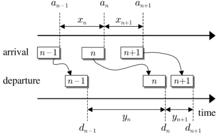
In this section, we build a simple model of a router that introduces random delay noise into the measurements of the receiver and use it to study the performance of packet-pair bandwidth-sampling techniques. Note that we depart from the common assumption of negligible and/or fluid cross-traffic and specifically aim to understand the effects of random queuing delays on the bandwidth sampling process. First consider an unloaded router with no cross-traffic. The packet-pair mecha-nism is based on an observation that if two packets arrive at the bottleneck link with spacing xsmaller than the transmission delay∆of the second packet over the link, their spacing after the link will be exactly∆. In practice, however, packets from other flows often queue between the two probe packets and increase their spacing on the exit from the bottleneck link to be larger than ∆.
Assume that packets of the probe traffic arrive to the bottleneck router at timesa1,a2, . . .and that inter-arrival times
an−an−1 are given by a random processxn determined by the server’s initial spacing. Further assume that the bottleneck node delays arriving packets by adding a random processing time ωn to each received packetn. For the remainder of the paper, we use constant1packet sizeqfor the probing flow and
arbitrarily-varying packet sizes for cross-traffic. Furthermore, there is no strict requirement on the initial spacingxnas long as the modeling assumptions below are satisfied. This means that both isolated packet pairs or bursty packet trains can be used to probe the path. Let the transmission delay of each application packet through the bottleneck link be q/C = ∆, whereCis the transmission capacity of the link. Under these assumptions, packet departure times dn are expressed by the following recurrence2:
dn =
a1+ω1+ ∆ n= 1
max(an, dn−1) +ωn+ ∆ n≥2. (2)
In this formula, the dependence of dn on departure time
dn−1is a consequence of FIFO queuing (i.e., packetncannot depart before packetn−1is fully transmitted). Furthermore, packet n cannot start transmission until it has fully arrived (i.e., timean). The value of the noise termωnis proportional to the number of packets generated by cross-traffic and queued
1Methods that vary the probing packet size also exist (e.g., [6], [10]). 2Times d
n specify when the last bit of the packet leaves the router. Similarly, timesanspecify when the last bit of the packet is fully received and the packet is ready for queuing.
zSuSd
arrival
departure
z[y[
zSuSdy
zr
[ztime
zLdSr
[zLdy
[zLd?
z?
zLdQ[
zSuSdQ
zQ
[zLd zu dS z[ zLdSFig. 1. Departure delays introduced by the node.
in front of packet n. The final metric of interest is inter-departure delay yn = dn −dn−1 as the packets leave the router. The various variables and packet arrival/departure are schematically shown in Figure 1.
Even though the model in (2) appears to be simple, it leads to fairly complicated distributions foryn if we make no prior assumptions about cross-traffic. We next examine several special cases and derive important asymptotic results about processyn.
III. RENEWALCROSS-TRAFFIC
A. Packet-Pair Analysis
We start our analysis with a rather common assumption in queuing theory that cross-traffic arrives into the bottleneck link according to some renewal process (i.e., delays between cross-traffic packets are i.i.d. random variables). In what follows in the next few subsections, we show that modeling of this direction requires stationarity (more specifically, ergodicity) of cross-traffic. However, since neither thei.i.d.assumption nor stationarity holds for regular Internet traffic, we then apply a different sampling methodology and a different analytical direction to derive a provably robust estimator of capacity C
and average cross-traffic rater¯.
The goal of bottleneck bandwidth sampling techniques is to queue probe packets directly behind each other at the bottle-neck link and ensure that spacingynon the exit from the router is ∆. In practice, however, this is rarely possible when the rate of cross-traffic is non-negligible. This does present certain difficulties to the estimation process; however, assuming a single congested node, the problem is asymptotically tractable given certain mild conditions on cross-traffic. We present these results below.
To generate measurements of the bottleneck capacity, it is commonly derived that the server must send its packets with initial spacing no more than∆(i.e., no slower thanC). This is true forunloadedlinks; however, when cross-traffic is present, the probes may be sent arbitrarily slower as long as each packet i arrives to the router before the departure time of packet i−1. This condition translates into an ≤ dn−1 and
(2) expands to:
dn=
a1+ω1+ ∆ n= 1
dn−1+ωn+ ∆ n≥2. (3)
From (3), packet inter-departure times yn after the bottle-neck router are given by:
yn=dn−dn−1= ∆ +ωn, n≥2. (4) Notice that random process ωn is defined by the arrival pattern of cross-traffic and also by its packet-size distribution. Since this process is a key factor that determines the distri-bution of sampled delays yn, we next focus on analyzing its properties. Assume that inter-packet delays of cross-traffic are given by independent random variables {Xi} and the actual arrivals occur at times X1, X1 +X2, . . . Thus, the arrival pattern of cross-traffic defines a renewal processM(t), which is the number of packet arrivals in the interval [0, t]. Using common convention, further assume that the mean inter-arrival delayE[Xi]is given by1/λ, whereλ= ¯ris the mean arrival rate of cross-traffic in packets per second.
To allow random packet sizes, assume that {Sj}, j =
1,2, . . .are independent random variables modeling the size of packets in cross-traffic. We further assume that the bottleneck link is probed by a sequence of packet-pairs, in which the delay between the packets within each pair is small (so as to keep their rate higher than C) and the delay between the
pairs is high (so as not to congest the link). Under these
assumptions, the amount of cross-traffic data received by the bottleneck link between probe packets 2m−1 and 2m (i.e., in the interval(a2m−1, a2m]) is given by a cumulative reward process:
vn=
M(an)−M(an−1)
j=1
Sj, n= 2m, (5) wherenrepresents the sequence number of the second packet in each pair. For now, we assume a general (not necessarily equilibrium) processM(t)and re-write (4) as:
yn= ∆ + vn C = ∆ + M(an)−M(an−1) j=1 Sj C , n= 2m. (6)
Since classical renewal theory is mostly concerned with limiting distributions,ynby itself does not lead to any tractable results because the observation period of the process captured by each of yn is very small.
Define a time-average processWnto be the average of{yi}
up to timen: Wn= 1 n n i=1 yi. (7)
Then, we have the following result.
Claim 1: Assuming ergodic cross-traffic, time-average
pro-cess Wn converges to: lim n→∞Wn= ∆ + λE[xn]E[Sj] C = ∆ +E[ωn], (8) R1 R2 Snd1 Snd2 1.5mb/s Rcv1 Rcv2 100mb/s 100mb/s 100mb/s 100mb/s
Fig. 2. Single-link simulation topology.
whereE[xn] is the mean inter-probe delay of packet-pairs.
Proof: Process Wn samples a much larger span of
M(t)and has a limiting distribution as we demonstrate below. Applying Wald’s equation to (6) [28]:
E[yn] = ∆ + E[M(an)−M(an−1)]E[Sj]
C . (9)
The last result holds since M(t) and Sj are independent and M(an) − M(an−1) is a stopping time for sequence {Sj}. Equation (9) can be further simplified by noticing that
E[M(t)] is the renewal functionm(t):
E[yn] = ∆ +(m(an)−m(an−1))E[Sj]
C . (10)
Assuming stationary cross-traffic, (10) expands to [28]:
E[yn] = ∆ + λE[xn]E[Sj]
C . (11)
Finally, assuming ergodicity of cross-traffic (which implies that of processyn), we can obtain (11) using a large number of packet pairs as the limit ofWn in (7) asn→ ∞.
Notice that the second term in (8) is strictly positive under the assumptions of this paper. This leads to an interesting observation that the filtering problem we are facing is quite challenging since the sampled process yn represents signal ∆ corrupted by a non-zero-mean noiseωn. This is a drastic departure from the classical filter theory, which mostly deals with zero-mean additive noise. It is also interesting that the only way to make the noise zero-mean is to either send probe traffic withE[xn] = 0(i.e., infinitely fast) or to have no cross-traffic at the bottleneck link (i.e.,λ= ¯r= 0). The former case is impossible sincexnis always positive and the latter case is a simplification that we explicitly want to avoid in this work. We will present our analysis of packet-train probing shortly, but in the mean time, discuss several simulations to provide an intuitive explanation of the results obtained so far.
B. Simulations
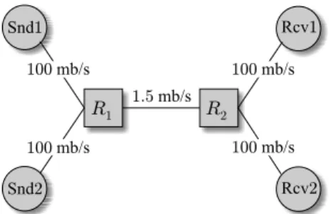
Before we proceed to estimation ofC, let us explain several observations made in previous work and put them in the context of our model in (6) and (8). For the simulations in this section, we used thens2network simulator with the topology shown in Fig. 2. In the figure, the source of probe packets
Snd1sends its data to receiver Rcv1across two routersR1
8 9 10 11 12 13 14 15 0 0.1 0.2 0.3 0.4 0.5 0.6 values of y(n) (ms) frequency (a)r¯= 1mb/s 10 15 20 25 0 0.1 0.2 0.3 0.4 values of y(n) (ms) frequency (b)r¯= 1.3mb/s
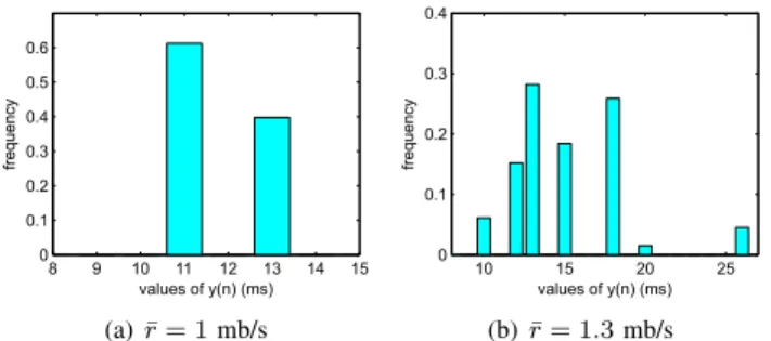
Fig. 3. The histogram of measured inter-arrival timesynunder CBR cross-traffic.
while the bottleneck linkR1→R2has capacityC= 1.5mb/s and 20 ms delay. Note that there are five cross-traffic sources attached toSnd2.
We next discuss simulation results obtained under UDP cross-traffic. In the first case, we initialize all five sources in Snd2 to be CBR streams, each transmitting at 200 kb/s (r¯ = 1 mb/s total cross-traffic). Each CBR flow starts with a random initial delay to prevent synchronization with other flows and uses 500-byte packets. The probe flow at Snd1
sends its data at an average rate of 500 kb/s for the probing duration, which results in 100% utilization of the bottleneck link. In the second case, we lower packet size of cross-traffic to 300 bytes and increase its total rate to 1.3 mb/s to demonstrate more challenging scenarios when there is packet loss at the bottleneck.
These simulation results are summarized in Fig. 3, which illustrates the distribution of the measured samples yn based on each pair of packets sent with spacingxn≤∆(the results exclude packet pairs that experienced loss). Given capacity
C = 1.5 mb/s and packet sizeq= 1,500 bytes, the value of ∆ is 8 ms. Fig. 3 shows that none of the samples are located at the correct value of 8 ms and that the mean of the sampled signal (i.e., Wn) has shifted to 11.7 ms for the first case and 14.5 ms for the second one.
Next, we employ TCP cross-traffic, which is generated by five FTP sources attached to Snd2. The TCP flows use different packet sizes of 540, 640, 840, 1,040, and 1,240 bytes, respectively. The histogram ofynfor this case is shown in Fig. 4 for two different average cross-traffic rates¯r= 750kb/s and ¯
r = 1 mb/s. As seen in the figure, even though some of the samples are located at 8 ms, the majority of the mass in the histogram (including the peak modes) are located at the values much higher than 8 ms.
Recall from (8) that Wn of the measured signal tends to ∆+E[ωn]. Under CBR cross-traffic, we can estimate the mean of the noise E[ωn]to be approximately11.7−8 = 3.7 ms in the first case and14.5−8 = 6.5ms in the second one. The two naive estimates of C based on Wn are C˜ =q/Wn = 1,025
kb/s and C˜ = 827kb/s, respectively. Likewise, for the TCP case, the measured averages (i.e., 12.2 and 13.3 ms each) of samples yn lead to incorrect naive estimates C˜ = 983 kb/s andC˜= 902 kb/s, respectively.
In order to understand how C˜ and the value ofWn evolve,
8 10 12 14 16 18 20 0 0.05 0.1 0.15 0.2 values of y(n) (ms) frequency (a) ¯r= 750kb/s 10 15 20 0 0.05 0.1 0.15 0.2 0.25 values of y(n) (ms) frequency (b)r¯= 1mb/s
Fig. 4. The histogram of measured inter-arrival timesynunder TCP cross-traffic.
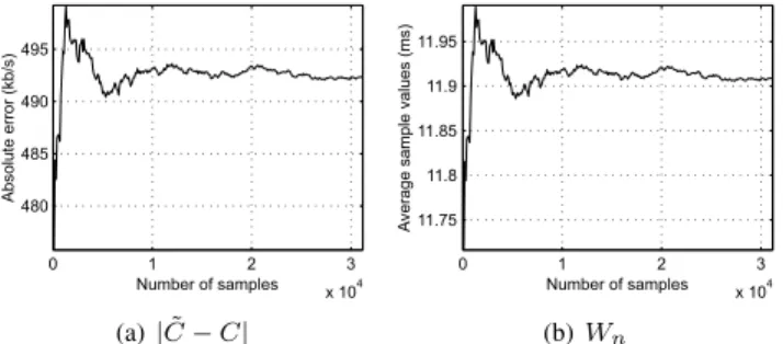
we run another simulation under 1 mb/s total TCP cross-traffic and plot the evolutions of the absolute error|C˜−C|and that of
Wn in Fig. 5. As Fig. 5(a) shows, the absolute error between
CandC˜ converges to a certain value after 5,000 samplesyn, providing a rather poor estimate C˜ ≈ 1,010 kb/s. Fig. 5(b) illustrates thatWn in fact converges to ∆ +E[ωn], where the mean of the noise isWn−∆≈11.9−8 = 3.9 ms.
Previous work [1], [4], [5], [15], [22] focused on identifying the peaks (modes) in the histogram of the collected bandwidth samples and used these peaks to estimate the bandwidth; however, as Figs. 3 and 4 show, this can be misleading when the distribution of the noise is not known a-priori. For example, the tallest peak on the right side of Fig. 3 is located at 13 ms (C˜ = 923kb/s), which is only a slightly better estimate than 827 kb/s derived from the mean ofyn. Moreover, the tallest peak in Fig. 4(a) is located at 14.5 ms, which leads to a worse estimateC˜ = 827kb/s compared to 983 kb/s computed from the mean ofyn.
To combat these problems, existing studies [1], [4], [5], [15], [22] apply numerous empirical methods to find out which mode is more likely to be correct. This may be the only feasible solution in multi-hop networks; however, one must keep in mind that it is possible thatnoneof the modes in the measured histogram corresponds to ∆ as evidenced by both graphs in Fig. 3.
C. Packet-Train Analysis
Another topic of debate in prior work was whether
packet-train methods offer any benefits over packet-pair methods.
Some studies suggested that packet-train measurements con-verge to the availablebandwidth3 for sufficiently long bursts
of packets [1], [4]; however, no analytical evidence to this effect has been presented so far. Other studies [5] employed packet-train estimates to increase the measurement accuracy of bottleneck bandwidth estimation, but it is not clear how these samples benefit asymptotic convergence of the estimation process.
We consider a hypothetic packet-train method that transmits probe traffic in bursts of k packets and averages the inter-packet arrival delays within each burst to obtain individual
3Even though this question appears to have been settled in some of the recent papers, we provide additional insight into this issue.
0 1 2 3 x 10⁴ 480 485 490 495 Number of samples Absolute error (kb/s) (a)|C˜−C| 0 1 2 3 x 10⁴ 11.75 11.8 11.85 11.9 11.95 Number of samples A verage sample values (ms) (b)Wn
Fig. 5. (a) The absolute error of the packet-pair estimate under TCP cross-traffic ofr¯= 1mb/s. (b) Evolution ofWn.
samples {Znk}, wheren is the burst number. For example, if
k= 10, samplesy2, . . . , y10defineZ110, samplesy12, . . . , y20
define Z210, and so on. The reason for excluding samples
y1, yn+1, . . . , ynk+1 is because they are based on the leading packets of each burst, which encounter large inter-burst gaps in front of them and do not follow the model developed so far.
In what follows in this section, we derive the distribution of {Znk} as k→ ∞.
Claim 2: For sufficiently large k, constant xn =x, and a
regenerative processesM(t), packet-train samples converge to the following Gaussian distribution for largen:
Znk−→D N ∆ +λxEC[Sj],λxV ar[Sj−λE[Sj]Xi] (k−1)C2 , (12) where −→D denotes convergence in distribution, N(µ, σ) is a Gaussian distribution with mean µ and standard deviationσ, andXi are inter-packet arrival delays of cross-traffic.
Proof: First, define ak-sample version of the cumulative
reward process in (5):
Vnk =
M(akn)−M(ak(n−1)+1)
j=1
Sj, n= 1,2, . . . . (13) Process Vnk is also a counting process, however, its time-scale is measured in bursts instead of packets. Thus, Vnk
determines the amount of cross-traffic data received by the bottleneck link during an entire burstn. Equation (13) shows that Znk can be asymptotically interpreted as the reward rate
of the reward-renewal process Vnk:
Znk= ∆ + V k n
(k−1)C, (14)
wherek−1 is the number of inter-packet gaps in ak-packet train of probe packets. AssumingM(t)is regenerative and for sufficiently largek, we have [28]:
Znk= ∆ + V k
1
(k−1)C +o(1). (15)
Applying the regenerative central limit theorem, constrain-ing the rest of the derivations in this section to constant
10 15 20 25 0 0.1 0.2 0.3 0.4 values of y(n) (ms) frequency (a)k= 5 10 15 20 25 0 0.1 0.2 0.3 0.4 0.5 values of y(n) (ms) frequency (b)k= 10
Fig. 6. The histogram of measured inter-arrival timesZnkbased on packet trains and CBR cross-traffic ofr¯= 1.3mb/s.
xn =x, and assuming E[Xi]<∞[28]: V1k k−1 D −→N λxE[Sj],λxV ar[Sj−λE[Sj]Xi] k−1 . (16) Combining (15) and (16), we get (12).
First, notice that the mean of this distribution is the same as that of samples {yn} in (11), which, as was intuitively expected, means that both measurement methods have the same expectation. Second, it is also easy to notice that the variance ofZnk tends to zero as long as V ar[Xi] is finite.
Claim 3: IfV ar[Xi] is finite, the variance of packet-train
samplesZnk tends to zero for largek.
Proof: Since λ,x, and E[Sj] are all finite and do not
depend on k, using independence of Sj and Xi in (12), we have: V ar[Znk] = λxV ar[Sj] +λ3xE2[Sj]V ar[Xi] (k−1)C2 2 , (17) which tends to 0 fork→ ∞.
As a result of this phenomenon, longer packet trains will produce narrower distributions centered at ∆ +E[ωn]. The CBR case already studied in Fig. 3(b) clearly has finite
V ar[Xi] and therefore samples {Znk} must exhibit decaying variance askincreases. One example of this convergence for packet trains withk= 5andk= 10is shown in Fig. 6.
D. Discussion
Now we address several observations of previous work. It is noted in [5] that while packet-pair histograms usually have many different modes, the histogram of packet-train samples becomes unimodal with increased k. This readily follows from (12) and the Gaussian shape of{Znk}. Previous
papers also noted (e.g., [5]) that as packet-train size k is increased, the distribution of samples {Znk} exhibits lower variance. This result follows from the above discussion and (17). Furthermore, [5] found that packet-train histograms for largektend to a single mode whose location is “independent of burst size k.” Our derivations provide an insight into how this process happens and shows the location of this “single mode” to be∆ +E[ωn] in (12).
In summary, packet-train samples{Znk}represent a limited reward rate that asymptotically converges to a Gaussian distri-bution with meanE[yn]. Perhaps it is possible to infer some
characteristics of{Xi}by observing the variance of{Znk}and applying the result in (12); however, since there are several unknown parameters in the formula (such as V ar[Xi] and
E[Sj]), this direction does not lead to any tractable results unless we assume a particular processM(t).
Since {Znk}asymptotically tend to a very narrow Gaussian distribution centered at ∆ +E[ωn], we find that there is no evidence that {Znk} measure the available bandwidth or offer any additional information about the value of∆ as compared to traditional packet-pair samples {yn}.
IV. ARBITRARYCROSS-TRAFFIC
In this section, we relax the stationarity and renewal as-sumptions about cross-traffic and derive a robust estimator of
C andr¯. Assume an arbitrary arrival processr(t) for cross-traffic, wherer(t)is its instantaneous rate at timet. We impose only one constraint on this process – it must have a finite time average ¯r shown in (1). The goal of the sampling process is to determine both C and ¯r. Since ¯r > C imply constant packet loss and zero available bandwidth, we are generally interested in non-trivial cases of r¯ ≤ C. Stochastic process
r(t)may be renewal, regenerative, a superposition of ON/OFF sources, self-similar, or otherwise. Furthermore, since packet arrival patterns in the current Internet commonly exhibit non-stationarity (due to day-night cycles, routing changes, link failure, etc.), our assumptions on r(t) allow us to model a wide variety of such non-stationary processes and are much broader than commonly assumed in traffic modeling literature. Next, notice that if the probing traffic can sampler(t)using a Poisson sequence of probes at times t1, t2, . . ., the average of r(ti)converges to r¯(applying the PASTA principle [28]):
lim n→∞ r(t1) +r(t2) +...+r(tn) n = limt→∞ 1 t t 0 r(u)du= ¯r, (18) as long as delaysτi=ti−ti−1 arei.i.d.exponential random variables. In order to accomplish this type of sampling, the sender must emit packet-pairs at exponentially distributed intervals. Assuming that the i-th packet-pair arrives to the router at time ti, it will sample a small segment of r(t) by allowinggi amount of data to be queued between the probes:
gi = ti+xi
ti
r(u)du≈r(ti)xi, (19) wherexiis the spacing between the packets in thei-th packet-pair. Again, assuming that yi is the i-th inter-arrival sample generated by the receiver, we have:
yi= ∆ + gi C = ∆ +
r(ti)xi
C . (20)
Finally, fixing the value of xi = x, notice that Wn has a
well-defined limit: lim n→∞Wn = nlim→∞ 1 n n i=1 ∆ + r(tCi)xi = ∆ + x Cnlim→∞ n i=1 r(ti) n = ∆ + xr¯ C. (21)
In essence, this result4 is similar to our earlier derivations,
except that (21) requires much weaker restrictions on cross-traffic and also shows that a single-node model is completely tractable in the setting of almost arbitrary cross-traffic. We next show how to extract bothC and¯rfrom (21).
A. Capacity
Observe that (21) is a linear function of x, where r¯is the slope and ∆is the intercept5. Therefore, by injecting
packet-pairs with two different spacingsxa andxb, one can compute the unknown terms in (21) using two sets of measurements {yai}and{yib}. To accomplish this, define the corresponding
average processes to beWna andWnb:
Wna = 1 n n i=1 yai, Wnb = 1 n n i=1 ybi. (22)
The simplest way to obtain both Wna and Wnb using a
single measurement is to alternate spacing xa and xb while
preserving the PASTA sampling property. Using a one-bit header field, the receiver can unambiguously sort the inter-arrival delays into two sets{yia}and{ybi}, and thus compute
their averages in (22).
While samples are being collected, the receiver has two running averages produced by (22). SubtractingWnbfromWna, we are able to separater/C¯ from∆:
lim n→∞(W a n −Wnb) = ( xa−xb)¯r C . (23)
Next, denote by∆˜n the following estimate of∆ at timen: ˜
∆n=Wna−xaW a n −Wnb
xa−xb . (24)
Taking the limit of (24), we have the following result.
Claim 4: Assuming a single congested bottleneck for which
time-average rater¯exists,∆˜n converges to ∆: lim n→∞∆˜n= ∆. (25) Proof: Re-writing (25): lim n→∞∆˜n= ∆ + xa¯r C −xa (xa−xb)¯r C(xa−xb) = ∆, (26)
which is obtained with the help of (21), (23), and (24). Our next result shows a more friendly restatement of the previous claim.
4A similar formula has been derived in [3], [8], [19] and several other papers under a fluid assumption.
5For technical differences between this approach and previous work (such as TOPP [19]), see [17].
TABLE I
AVAILABLEBANDWIDTHESTIMATIONERROR
Bottleneck capacity Relative error
C(mb/s) Model (29) Pathload Spruce IGI
1.5 8.6% 46.5% 27.9% 84.5%
5 8.3% 40.1% 23.4% 90.0%
10 10.1% 40.9% 26.9% 89.0%
15 7.7% 38.5% 24.5% 83.1%
Corollary 1: Assuming a single congested bottleneck for
which time-average rate r¯ exists, estimate C˜n = q/∆˜n
converges to capacity C: lim n→∞C˜n = nlim→∞ q Wna−xaWna−Wnb xa−xb = lim n→∞ q(xa−xb) xaWnb−xbWna =C. (27) B. Available Bandwidth
Notice that knowing an estimate of C in (27) and using r¯
in (23), it is easy to estimate the mean rate of cross-traffic: lim
n→∞
(Wna−Wnb) ˜Cn
xa−xb = ¯r, (28)
which leads to the following result.
Corollary 2: Assuming a single congested bottleneck for
which time-average rate r¯exists, the following converges to the available bandwidth A=C−r¯:
lim n→∞q xa−xb−Wna+Wnb xaWnb−xbWna =C−r¯=A. (29) C. Simulations
We confirm these results and compare our models with several recent methodsspruce[26], IGI [8], andpathload
[12] through ns2 simulations. Since the main theme of this paper is bandwidth estimation in heavily-congested routers, we conduct all simulations over a loaded bottleneck link in Fig. 2 with utilization varying between 82% and 92% (the exact value changes depending on C and the interaction of TCP cross-traffic with probe packets). Delays xa andxb are set to maintain the desired range of link utilization.
Define EA = |A˜ −A|/A and EC = |C˜ − C|/C to be the relative estimation errors of A and C, respectively, where A is the true available bandwidth of a path, A˜ is its estimate using one of the measurement techniques, C is the true bottleneck capacity, and C˜ is its estimate. Table I shows relative estimation errors EA for spruce, IGI, and
pathload. For pathload, we averaged the low and high
values of the produced estimates A˜. In the IGI case, we used the estimates available at the end of IGI’s internal convergence algorithm. Also note that we fed both spruce and IGI the exact bottleneck capacityC, while model (29) andpathload
operated without this information.
As the table shows, spruce performs better than
pathload in heavily-congested cases, which is expected
0 200 400 600 800 1000 1200 0 0.5 1 1.5 Number of samples Relative estimation error (a) EC 0 200 400 600 800 1000 1200 0 0.2 0.4 0.6 0.8 Number of samples Relative estimation error (b)EA
Fig. 7. Evolution of relative estimation errors of (27) and (29) over a single congested link withC= 1.5mb/s and 85% link utilization.
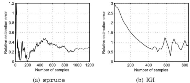
0 200 400 600 800 1000 1200 0 0.2 0.4 0.6 0.8 1 1.2 Number of samples Relative estiamtion error (a)spruce 200 400 600 800 0 0.5 1 1.5 2 2.5 3 Number of samples Relative estimation error (b) IGI
Fig. 8. Relative estimation errorsEAproduced byspruceand IGI over a single congested link withC= 1.5mb/s and 85% link utilization.
since it can utilize the known capacity information. Inter-estingly, however, IGI’s estimates are worse than those of
pathload even though IGI utilizes the true capacity C in
its estimation algorithm. A similar result is observed in [26] under a relatively small amount of cross-traffic (20% to 40% link utilization).
Next, we examine models (27), (29) with a large number of samples to show their asymptotic convergence and estimation accuracy. We plot the evolution of relative estimation errors
EC andEA in Fig. 7. As Fig. 7(a) shows,C˜ converges to a value that is very close (within 3%) to the true value ofC. In Fig. 7(b), the available bandwidth estimates quickly converge within 10% of A. For the purpose of comparison, we next plot estimation errors EA produced by spruce and IGI in Fig. 8. As Fig. 8(a) shows, even with the exact value of C
and after 1,000 samples, spruceexhibits an error of 27%. Furthermore, IGI’s estimates are much worse thanspruce’s as illustrated in Fig. 8(b), which plots the evolution of errors until IGI’s internal algorithm terminates.
To better understand these results, we next study how the accuracy of capacity information provided tospruceand IGI affects their measurement accuracy.
D. Further Analysis ofspruceand IGI
Since bottleneck capacities of Internet paths are not gener-ally known, the use ofspruceand IGI may be limited to a small number of known paths, unless these methods can obtain capacity measurements from other tools such as nettimer
[15], [16],pathrate[5], or CapProbe [13]. These estimators ofCare usually very accurate when the routers along the path are not highly utilized; however, as link utilization increases,
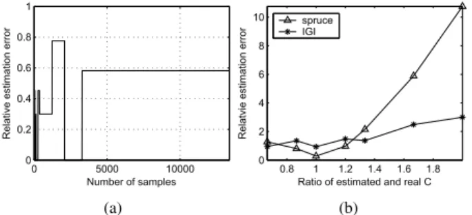
0 5000 10000 0 0.2 0.4 0.6 0.8 1 Number of samples Relative estimation error (a) 0.8 1 1.2 1.4 1.6 1.8 0 2 4 6 8 10
Ratio of estimated and real C
Relatvie estimation error spruce IGI (b)
Fig. 9. (a) Relative capacity estimation errorECmeasured by CapProbe. (b) Relative estimation errorsEAofspruceand IGI based on the ratioC/C˜ .
their results often become inaccurate. Hence, a natural ques-tion is how robust arespruceand IGI to inaccurate values
of C provided to their estimation process? We examine this
issue below, but first discuss simulation results of CapProbe to illustrate the pitfalls that many estimators of C experience over heavy-loaded bottleneck links.
For the CapProbe simulation, we use the topology shown in Fig. 2 with a single bottleneck link whose utilization was kept at 85% using five TCP cross-traffic sources. Fig. 9(a) plots the evolution ofECproduced by CapProbe in this experiment. As the figure shows, CapProbe’s minimum filtering is sensitive to random queuing delays in front of the first packet of the pair and can eventually converge to a completely wrong value (60% error).
We next examine how the value of C˜ = C supplied to IGI and spruce affects their accuracy. We plot the relative estimation errors in Fig. 9(b), in which the accuracy of both methods deteriorates whenC/C˜ becomes large. To understand the exact effect ofC˜ on these methods, we have the following simple analysis.
According to [8], IGI first sends packet trainsZiwith inter-packet spacingxi(xi < xjfori < j) to determine theturning
point xˆ. Each packet-train consists of kback-to-back packets
and the turning point is the n-th inter-packet spacing xn at which the receiving rate of probe traffic starts to match the sending rate: ˆ x=xn= 1 k−1 k i=2 yi. (30)
Subsequently, IGI computes the average cross-traffic rate r¯
as following [8]: ¯ r= yi>max(∆,xˆ) ˜ C(yi−∆) (k−1)ˆx (31)
and estimates available bandwidth by subtracting (31) from its a-priori known value of C˜: A˜ = ˜C −¯r. Notice from (31) that the average cross-traffic r¯ depends on the capacity value provided to the estimation algorithm. This dependency explains the increased estimation inaccuracy when C/C˜ = 1
as illustrated in Fig. 9(b).
Similarly, estimation accuracy of sprucealso changes as a function ofC˜. For example, even thoughspruceprovides
0 10 20 30 40 0 10 20 30 40 x(n) (ms) mean of y(n) (ms) Simulation result y=x (a) CBR cross-traffic 0 20 40 60 80 100 0 20 40 60 80 100 x(n) (ms) mean of y(n) (ms) Simulation result y=x (b) TCP cross-traffic Fig. 10. Convergence ofωnto zero-mean additive noise for largexnunder CBR and TCP cross-traffic.
better estimates than IGI with a correct capacity value C˜ = C= 1.5 mb/s, it exhibits large estimation errors (over 200%) whenC˜ exceeds C by33%. This means that the accuracy of
spruceis also heavily dependent on the performance of the
underlying bottleneck bandwidth estimation method.
To better understand this observation, we next analyze
spruce’s estimation process. Spruce collects individual
samplesAi [26]: Ai=C 1−yi−∆ ∆ , (32)
whereyi is the i-th measured packet spacing at the receiver. The algorithm averages samples Ai to obtain a running esti-mate of the available bandwidth:
An= 1 n n i=1 Ai = 2C−C 2 qn n i=1 yi. (33)
Taking the limits of (33) and substituting Wn from (21) into (33), we get ˜ A= lim n→∞An=C− x ∆¯r. (34)
This brief analysis shows that the bandwidth estimation mechanism inspruce requires that the sender set its inter-packet spacing x to be ∆ = q/C. This is possible when C
is known exactly; however, in cases when C is not correctly estimated, the initial spacingxcannot be set to∆andspruce
cannot converge toA. Also notice that ifr¯C, estimation er-rors are generally small; however, as link utilization increases, any deviation of x/∆ from 1 will have a significant impact onA˜.
V. MULTIPLELINKS
In this section, we extend our single-node model to the case of multiple congested routers and conjecture that it is impossible to derive a closed-form solution that filters out the noise introduced by cross-traffic at several links of an end-to-end path.
A. Large Inter-Probe Delays
Consider the original model of a router in (2). This time, assume thatnoneof the probe packets queue behind each other at the bottleneck router. This means that packetn−1 leaves
R0 R2 Snd1 Snd3 Cp Rcv1 Rcv2 100mb/s 100mb/s 100mb/s 100mb/s R1 Rcv3 Snd2 C 100mb/s 100mb/s
Fig. 11. Multi-link simulation topology.
the router before packetn arrives, which is expected if inter-packet spacing xn at the source is very large compared to the transmission delay ∆. Under these assumptions, dn−1 < an
and (2) becomes:
dn =an+ωn+ ∆, n≥1. (35) Hence, inter-departure delays yn are:
yn=an−an−1+ωn−ωn−1, n≥2. (36) Notice that the first terman−an−1in (36) is the inter-arrival delay xn of the probe traffic and the second termωn−ωn−1
can be modeled as some zero-mean random noise. This can be explained intuitively by noticing that under the assumption of large xn, each router delays probe packets (on average) by the same amount. Then the distance between each pair of subsequent packets fluctuates around the mean of xn. Using an inductive argument, it is also easy to show the following.
Claim 5: If the initial spacingxn is larger (in a statistical
sense) than queuing delays experienced by packets at each router of anN-hop end-to-end path, the mean of the sampled signal yn is equal to E[xn] and the following holds for each routerj:
E[ωn(j)−ωn(j−)1] = 0. (37) To confirm that the zero-mean model in (37) holds in practice, we run ns2simulations with 85% utilization at the bottleneck link and varying packet sizes of CBR and TCP cross-traffic. The plots of E[yn] as a function of xn for different values of xn = x are shown in Fig. 10. As the two figures show, E[yn] converges to xn at 40 and 100 ms, respectively, at which time the noise at the bottleneck router becomes zero-mean-additive. Note that similar results hold for multiple congested routers, different traffic patterns, and different packet sizes. Also note that the point at whichE[yn]
converges to x is not necessarily the value of the available bandwidth as was suggested in prior work [8].
B. Recursive Model for Multi-Node Paths
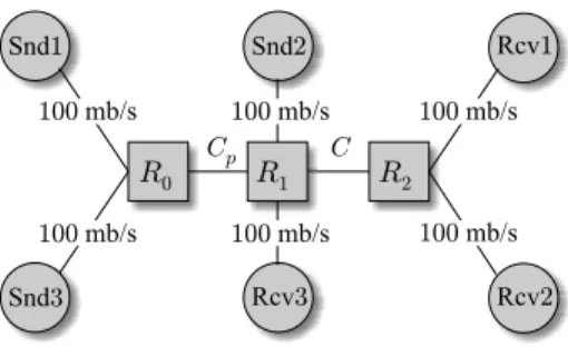
Assuming multiple congested routers along a path, the result in (25) no longer holds. To better understand multi-link effects, we use the topology in Fig. 11, where the bottleneck link C
has capacity 1.5 mb/s and pre-bottleneck linkCp = 1.8mb/s. Five FTP sources are attached to each of snd2 and snd3
0 0.5 1 1.5 2 x 10⁴ 7.5 8 8.5 9 Number of samples T ransmission delay (ms) estimatedD D
(a) Single congested link
0 0.5 1 1.5 2 x 10⁴ 8 9 10 11 12 13 Number of samples T ransmission delay (ms) estimatedD D
(b) Two congested links Fig. 12. The evolution of estimated transmission delay∆n˜ for a single and two congested links.
and both links are utilized by cross-traffic at 85%. Fig. 12 illustrates the convergence process of ∆˜n for the single-node and multi-node cases. As Fig. 12(b) shows, estimates∆˜n do not converge to the true value of∆ = 8ms, regardless of the number of samplesyi.
Notice that it is possible to recursively extend the original model in (26) to multiple congested links where the inputxn
of each link is the output yn of the previous link. However, this model becomes intractable as we show next. Add index
j to each process and each random variable to indicate that it is local to router j along the path from the sender to the receiver. Further assume that Q(ij) is the queuing delay (due to cross-traffic and other probe packets) in front of packet i
inside router j and φ(ij) is some zero-mean noise process at router j at time i. Then, we define the following recursive model: yi(j)= ∆j+ωi(j), xi(j)< Q(ij−)1 ∆j+φ(ij), xi(j)≥Q(ij−)1 , (38)
wherey(ij)is the departure spacing of thei-th packet-pair from router j, ∆j = q/Cj is the transmission delay of the probe packets over linkj, andx(ij)is the arrival spacing between the probes at routerj. Notice that if the arrival spacing between packets i−1 andi (which is simply xi(j) = yi(j−1)) is less than the time packet i−1 spends in the buffer (i.e., Q(ij−)1), the two packets queue behind each other and follow the model developed earlier in this paper. When the opposite holds, the packets do not queue behind each other and the router adds
i.i.d.zero-mean noiseφ(ij) to∆j.
C. Conjecture of Impossibility
One of the main difficulties of this situation is the stochastic mixture of the two types of noise in (38). While at this time we do not offer a complete treatment of this problem, we show thatevenwhen all links follow the first model (i.e., all packets queue behind each other), the problem appears intractable. Under these assumptions, (38) leads to:
Wn(j)= ∆j+ 1 nCj n i=1 rj(ti)x(ij), (39)
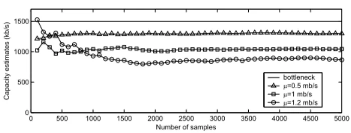
0 500 1000 1500 2000 2500 3000 3500 4000 4500 5000 0 500 1000 1500 Number of samples Cap acity estimates (kb/s) bottleneck m=0.5 mb/s m=1 mb/s m=1.2 mb/s
Fig. 13. Evolution of estimated bandwidth for two congested links.
whererj(t)is the cross-traffic process at router j. For a two congested-router case, (39) becomes:
Wn(2) = ∆2+ 1 nC2 n i=1 r2(ti)yi(1) = ∆2+nC1 2 n i=1 r2(ti) ∆1+r1(Cti)x 1 → ∆2+∆C1¯r2 2 + x C1C2 ∞ 0 r1(u)r2(u)du. (40) Since Poisson samples taken at the receiver lead to obtaining a time average of a mixed signal introduced by the two routers, it appears impossible to filter out the unknown cross-traffic statistics or the main integral in (40).
We next examine how the amount of cross-traffic in two congested links affects the estimation accuracy of the earlier models developed in the paper. We set the average cross-traffic rates r1(t) and r2(t) to be the same in both routers (i.e., ¯r1 = ¯r2 = µ) and vary this value between 500 kb/s and 1.2 mb/s. We again use the topology in Fig. 11 and plot in Fig. 13 the value of C˜n computed using (27) when cross-traffic is simultaneously injected into both links (Cp= 2mb/s,
C = 1.5 mb/s). As the figure illustrates, the estimates of the bottleneck bandwidth converge to a value that is significantly less than the true capacityC and become progressively worse as µincreases.
VI. CONCLUSION
This paper examined the problem of estimating the capac-ity/available bandwidth of a single congested link and showed a simple stochastic analysis of the problem. Unlike previous approaches, our estimation didnot rely on empirically-driven methods, but instead used a queuing model of the bottle-neck router that specifically assumed non-negligible, non-fluid cross-traffic. It is also the first model to provide simultaneous asymptotically-accurate estimation of both C and A in the presence of arbitrary cross-traffic.
Our analysis in the multi-node cases suggests that the problem of obtaining provably-convergent estimates ofCand
Ain such environments does not have a solution. This insight possibly explains the lack of analytical/stochastic justification for many of the proposed methods. Knowing that accurate estimation of C for the multi-node case is impossible will potentially provide an important foundation for the methods that rely on empirically-optimized heuristics.
REFERENCES
[1] B. Ahlgren, M. Bj¨orkman, and B. Melander, “Network Probing Using Packet Trains,”Swedish Institute Technical Report, March 1999. [2] M. Allman and V. Paxson, “On Estimating End-to-End Network
Param-eters,”ACM SIGCOMM, August 1999.
[3] J. Bolot, “End-to-End Packet Delay and Loss Behavior in the Internet,”
ACM SIGCOMM, September 1993.
[4] R.L. Carter and M.E. Crovella, “Measuring Bottleneck Link Speed in Packet Switched Networks,”International Journal on Performance Evaluation27 & 28, 1996.
[5] C. Dovrolis, P. Ramanathan, D. Moore, “What Do Packet Dispersion Techniques Measure?”IEEE INFOCOM, April 2001.
[6] A.B. Downey, “Using PATHCHAR to Estimate Internet Link Charac-teristics,”ACM SIGCOMM, August 1999.
[7] K. Harfoush, A. Bestavros, and J. Byers, “Measuring Bottleneck Band-width of Targeted Path Segments,”IEEE INFOCOM, March 2003. [8] N. Hu and P. Steenkiste, “Evaluation and Characterization of Available
Bandwidth Probing Techniques,” IEEE Journal on Selected Areas in Communications, vol. 21, No. 6, August 2003.
[9] V. Jacobson, “Congestion Avoidance and Control,”ACM SIGCOMM, 1988.
[10] V. Jacobson, “pathchar – A Tool to Infer Characteristics of Internet Paths,” ftp://ftp.ee.lbl.gov/pathchar/.
[11] M. Jain and C. Dovrolis, “End-to-End Available Bandwidth: Measure-ment Methodology, Dynamics, and Relation with TCP Throughput,”
ACM SIGCOMM, 2002.
[12] M. Jain and C. Dovrolis, “Pathload: A Measurement Tool for End-to-End Available Bandwidth,” Passive and Active Measurements (PAM) Workshop, 2002.
[13] R. Kapoor, L. Chen, L. Lao, M. Sanadidi, and M. Gerla, “CapProbe: a Simple and Accurate Capacity Estimation Technique,”ACM SIGCOMM, August 2004.
[14] S. Keshav, “A Control-Theoretic Approach to Flow Control,” ACM
SIGCOMM, 1991.
[15] K. Lai and M. Baker, “Measuring Bandwidth,”IEEE INFOCOM, 1999. [16] K. Lai and M. Baker, “Measuring Link Bandwidths Using a
Determin-istic Model of Packet Delay,”ACM SIGCOMM, August 2000. [17] X. Liu, K. Ravindran, B. Liu, and D. Loguinov, “Single-Hop Probing
Asymptotics in Available Bandwidth Estimation: A Sample-Path Anal-ysis,”ACM IMC, October 2004.
[18] B.A. Mah, “pchar: A Tool for Measuring Internet Path Characteristics,” http://www.employees.org/∼bmah/ Software/ pchar/, June 2001. [19] B. Melander, M. Bj¨orkman, P. Gunningberg, “A New End-to-End
Probing and Analysis Method for Estimating Bandwidth Bottlenecks,”
IEEE GLOBECOM, November 2000.
[20] A. Pasztor and D. Veitch, “Active Probing using Packet Quartets,”ACM IMW, 2002.
[21] A. Pasztor and D. Veitch, “The Packet Size Dependence of Packet Pair Like Methods,”IEEE/IFIP IWQoS, 2002.
[22] V. Paxson, “Measurements and Analysis of End-to-End Internet Dy-namics,”Ph.D. dissertation, Computer Science Department, University of California at Berkeley, 1997.
[23] S. Ratnasamy and S. McCanne, “Inference of Multicast Routing Trees and Bottleneck Bandwidths using End-to-End Measurements,” IEEE
INFOCOM, March 1999.
[24] V. Ribeiro, R. Riedi, R. Baraniuk, J. Navratil, and L. Cottrell, “pathChirp: Efficient Available Bandwidth Estimation for Network Paths,”Passive and Active Measurements (PAM) Workshop, 2003. [25] D. Sisalem and H. Schulzrinne, “The Loss-delay Based Adjustment
Algorithm: A TCP-friendly adaptation scheme,” IEEE Workshop on Network and Operating System Support for Digital Audio and Video (NOSSDAV), 1998.
[26] J. Strauss, D. Katabi, and F. Kaashoek, “A Measurement Study of Available Bandwidth Estimation Tools,”ACM IMC, 2003.
[27] R. Wade, M. Kara, and P.M. Dew, “Study of a Transport Protocol Employing Bottleneck Probing and Token Bucket Flow Control,”IEEE ISCC, July 2000.
[28] R.W. Wolff, “Stochastic Modeling and the Theory of Queues,” Prentice-Hall, 1989.