Motion Planning for Omnidirectional Dynamic Gait
in Humanoid Soccer Robots
J.J. Alcaraz-Jim´enez, D. Herrero-P´erez, and H. Mart´ınez-Barber´a
Abstract—This paper deals with the problem of planning the Center of Mass (CoM) trajectory of a humanoid robot while its feet follow an omnidirectional walking pattern. This trajectory should satisfy the dynamic stability criterion to ensure analyti-cally that the Zero Moment Point (ZMP) lies within the support polygon. The proposed approach provides flexibility and agility to humanoid robots, which is of special interest in highly dynamic environments, such as soccer robotics. The experimental results show that the proposed method permits on-line calculation of omnidirectional stable trajectories in the commercial humanoid platform NAO, which has limited computational resources.
Index Terms—Humanoid Soccer Robots, Omnidirectional Lo-comotion, Dynamic gait, RoboCup.
I. INTRODUCTION
A
N IMPORTANT feature that provides flexibility and simplifies drastically the control of mobile robots is omnidirectional locomotion, of special interest in dynamic environments. Omnidirectional locomotion provides the robot with the ability to modify its motion quickly, independently of its bearing, which is very useful when environmental con-ditions change. Moreover, it facilitates hardware abstraction, allowing us to reuse high level controllers and behaviors from other developments. When possible, omnidirectional drives have been employed in diverse platforms to facilitate robot control.One interesting example is the Robocup competition. The different Robocup leagues have incorporated omnidirectional drives to facilitate the control of the robots and to provide the capabilities for kicking the ball accurately. The reason is that using an omnidirectional drive makes it easier to locate the robots in specific positions for kicking in the proper direction. Some examples in different leagues are omnidirectional drive for Small-Size League [1], past Sony Four-Legged League [2], legged-robots in Rescue League [3] and humanoid robots [4]. The most popular and simple schemes to control walking bipeds are trajectory tracking methods [5], which solve the motion dynamics equations to calculate offline trajectories for individual joints keeping the ZMP within the support polygon [6]. The main shortcomings of these approaches are as follows:
• There is only a finite set of gaits computed off-line. • They require precise robot and environment models.
• Robustness under relative high disturbances is not en-sured by tracking approaches.
• Dynamic equations with many degrees of freedom and trajectory tracking can be computationally expensive. J.J. Alcaraz-Jim´enez, D. Herrero-P´erez, and H. Mart´ınez-Barber´a are with the Department of Information and Communications Engineering, University of Murcia, 30100 Espinardo, Murcia, Spain.
E-mail: [email protected], [email protected] and [email protected]
The simplified models are used to calculate CoM trajectories and introduce feedback control. The most popular model is the inverted pendulum simplification [7], which represents humanoid dynamics by its Center of Mass (CoM) connected by a massless telescopic leg to the supporting foot. Some variants model sagittal and frontal components by means of more than one inverted pendulum [8], representing different linked parts of humanoid robots. On the other hand, central pattern generators [9] [10] need neither a robot dynamic model nor an environment model. They aim to imitate biological neural circuits that can produce rhythmic patterns without receiving rhythmic inputs.
In spite of capabilities that can incorporate omnidirectional locomotion to bipeds, some advanced developments are still controlled by pre-computed trajectories, with the feedback focused on tracking these routes and ensuring stability un-der slight disturbances. These trajectories cannot be coupled because they usually do not match up and smoothness is not ensured. Consequently, the robot has to stop in order to track a new trajectory.
The online CoM trajectory generation for omnidirectional dynamic gaits has also been studied in several ways. Recent developments [4] aim to address this problem by ignoring the ZMP position and employing empirical sinusoidal equations instead. When CoM trajectory generation is based on ZMP a precise model of the robot is required. For example, the problem can be formulated as a ZMP tracking servo controller [11]. Although this approach has been successfully tested in the Robocup environment [12], it assumes some error in CoM trajectory generation, which is decreased by adding future information about ZMP position. Finally, an analytical solution for CoM trajectory generation problem based on ZMP is proposed in [13]. However, effectiveness of the approach is compromised by fast changes in the expected position of the feet.
The flexibility provided by omnidirectional locomotion and the accuracy of online analytical approaches are the motivation for this paper, which proposes an analytical method for plan-ning the CoM trajectories of an omnidirectional dynamic gait for biped robots. This problem was previously addressed by [13]. The main difference with the proposed approach is that a different set of parameters and a tuning criterion are proposed in order to improve the precision of ZMP trajectories.
The paper is structured as follows. Section II introduces the problem and the proposed approach. Section III describes the walking pattern generation approach adopted to plan omnidirectional trajectories. Section IV presents the boundary conditions employed to trace trajectories in any direction. The experimental validation is presented in Section V, and finally,
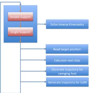
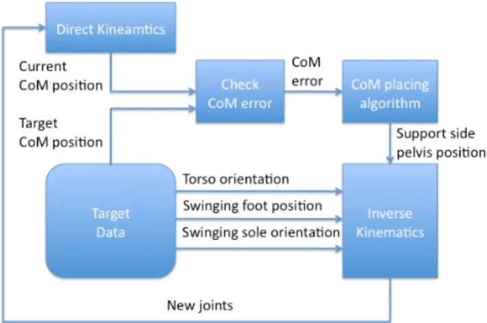
Fig. 1. Overview of the locomotion system.
some conclusions are presented in Section VI. II. OMNIDIRECTIONALLOCOMOTION
The proposed locomotion system is based on position control, i.e. the humanoid robot is commanded by a target position and the locomotion system generates the sequence of joint positions to reach such a target location. Through a local coordinate system fixed to the hip of the robot, the target position consists of the relative target position, the relative target orientation, and the feet layout relative to the target reference.
The target position can be modified at any time in order to provide flexibility and reactivity to the robot control. When the target position is modified the sequence of joint positions is recalculated taking into account the stability criterion for humanoid robots. The locomotion problem can be divided into four steps:
1) Finding the target position of the swinging foot given the target position for the feet.
2) Planning the trajectory of the swinging foot for one step. 3) Planning the CoM trajectory to move the swinging foot one step considering single support time and target position.
4) Finding the sequence of joint positions to follow both CoM and swinging foot trajectories.
Fig. 1 shows the different stages of the locomotion system. We can observe that the inverse kinematics processing is the only stage executed at every cycle, which helps to maintain the CPU consumption at a low level. The trajectories for the swinging foot and the CoM are only calculated when a single support stage is finished, and thus robot reactivity is limited to time to walk one step. Reactivity, which is a key issue in robotic soccer, is increased by using short and fast steps.
III. MOTION PLANNING
The omnidirectional locomotion problem can be formulated as finding the CoM and feet trajectories to move the robot
stability criterion for humanoid robots. Two approaches can be employed to determine the stability of the robot: static and dynamic balance criteria.
The static balance criterion assumes that only the gravita-tional force is acting on the robot, hence keeping the vertical CoM projection on the support polygon ensures stability. The support polygon is the paw area of the supporting foot contacting with the floor in single-support stage, while it is the convex hull including the paw areas of both feet in the double-support stage. However, the inertia forces should be negligible, in order to ensure stability. This can be achieved with static balance, but it gives rise to a slow gait.
On the other hand, dynamic balance takes into account both gravitational force and inertia. Normally, the Zero Moment Point (ZMP) is employed to determine the dynamic balance. The ZMP specifies the point with respect to which dynamic reaction forces at the contact of the foot with the ground do not produce any momentum. The dynamic balance condition consists of the ZMP projection on the ground lies within the convex hull. When ZMP projection on the ground is out of the convex hull, ZMP is calledFictitious Zero Moment Point
(FZMP).
Humanoid gaits usually differentiate between single-support stage (robot standing on only one foot) and double-support stage (both feet on the ground). In order to walk, the robot has to move its legs from double-support stage to single-support stage, alternating between legs. The proposed approach aims to maintain the ZMP in the center of the supporting foot during the single-support stage and to avoid the ZMP leaving convex hull during the double-support stage.
A. Inverted Pendulum model
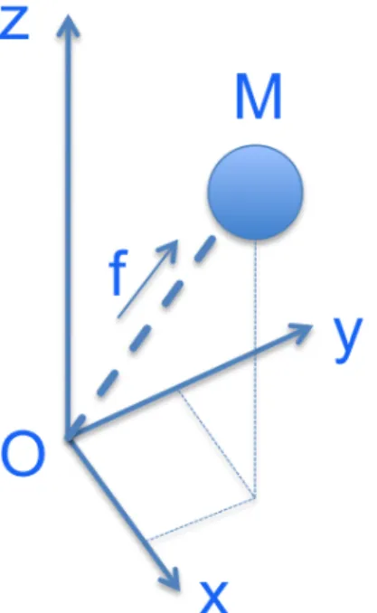
The 3D Linear Inverted Pendulum Model (3D-LIMP) [14] is used to plan the CoM motion given the ZMP position. Fig. 2 shows this simplified robot model as a single point located at the CoM where all the mass of the robot is concentrated. Such a point is connected to the ground by a massless support leg whose length can be modified. The entire model behaves as an inverted pendulum, turning freely around the supporting point, which is the place where the combination of inertia and gravity forces projects on the floor.
The CoM trajectories are planned considering that the supporting point is located at the ZMP of the humanoid robot (stability criterion). The 3D-LIMP model only considers the propulsion force and the gravity. The former force, applied to the point representing the mass of the robot, can be decomposed into, fx = ( x r)f (1) fy = ( y r)f (2) fz = ( z r)f (3)
wherefx,fy andfz are the Cartesian components of propul-sion force andris the distance between the supporting point
Fig. 2. Inverted Pendulum model.
and the CoM. By adding the gravity to the system, the motion equations defining the movement of the CoM are as follows,
Mx¨ = (x r)f (4) My¨ = (y r)f (5) Mz¨ = (z r)f−M g (6)
These motion equations are simplified by constraining the CoM movement to the planeXY at a height as follows,
z=kxx+kyy+zc (7) wherezcis the point where the planeXY intersects thezaxis, and kx andky are the slopes of the trajectory constrained to such an XY plane. The forces applied to the model should be orthogonal in order to ensure that the CoM remains in this plane. This fact is described as follows,
f(x r) f( y r) f( z r)−M g × −kx −ky 1 = 0 (8)
By replacing z using the expression (7), we obtain the following equation for the propulsion force applied to the CoM,
f = M gr
zc
(9) which should be proportional to the leg length. In addition, it decreases with the height of the CoM. This force can be replaced in (4) and (5) in order to obtain the relationship between the acceleration that should be applied to the CoM and the distance to the supporting point.
¨ x = xg zh (10) ¨ y = y g zh (11) which can be expressed from the system reference centered at the support point (px, py) as follows,
¨ x= (x−px) g zh (12) ¨ y= (y−py) g zh (13) This is the simplified robot model used for planning the trajectories of the CoM to ensure stability. The following sections describe the strategy adopted to plan omnidirectional trajectories for biped dynamic gait using these simplifications.
B. Trajectory planning
In order to satisfy the stability criterion during the single-support stage, the ZMP position should be approximately constant. In particular, the ZMP should be located in the convex hull defined by the sole of the supporting leg that is in contact with the floor. Thus, px and py are considered time independent and the previous differential equations can be solved by using the following expression for the CoM movement,
x(t) =c1xeαt+c2xe−αt+px (14)
y(t) =c1yeαt+c2ye−αt+py (15) whereα=qzg
h is a constant defined for simplification. These expressions can be used to plan the CoM trajectory that locates the ZMP at some target position. In order to gener-ate a walking pattern, we only have to link these trajectories by moving the ZMP alternatively between feet. However, these kind of CoM trajectories induce large modifications of the ZMP due to the acceleration of the CoM. In other words, strong accelerations make the effect of body link deformation of humanoid robots stronger. Besides, the simplified robot model becomes less accurate when high accelerations exist, which is why the CoM acceleration should be minimized.
The CoM accelerations following the walking pattern can be minimized by using both planning and control based tech-niques. We have adopted the simple approach of introducing a double-support stage between single-support stages, which decreases the CoM accelerations induced by single-support stages. The double-support stage is introduced by defining the expression that moves the CoM from the position where it finished the last single-support stage to the position where it starts the next single-support stage. In order to ensure speed continuity an expression of four variables, two variables for speed and two variables for position boundary conditions, is chosen to represent the double-support trajectory as follows,
x(t) =c3xt3+c4xt2+c5xt+c6x (16)
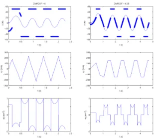
Fig. 3. Comparison between a pure single-support gait (left) and a typical gait with a double-support stage (right). The first row shows a curve with the lateral evolution of the CoM together with the position of the ZMP (thick points). Second and third rows show the lateral speed and acceleration of the CoM respectively.
where CoM speed and acceleration profiles can be obtained as first and second derivative of CoM trajectory.
The double-support stage decreases the CoM acceleration between single-support stages and fixes a top for the maximum speed, removing the peaks that would occur in the transition from one support-foot to the next one in a pure single-support gait. The larger this double support area, the lower the CoM acceleration during the transition from one support-foot to the next. However, a larger double-support stage means the robot takes a longer time for each step, resulting in a slower global speed. In order to tune the behavior of our gait in this aspect, the ZM P DSF parameter can be used.
C. Discussion
During single-support stages, the ZMP stays still at one point of the supporting-foot, while in the double-support stage, the ZMP has to travel from one foot to the other. The amount of space between the feet that will be used for the ZMP during its trip from one support-foot to the following one can be specified. In our approach, this amount of space is specified as a fraction of the total amount of space between the feet, and this fraction is theZM P DSF.
Fig. 3 shows the influence of ZM P DSF parameter for pure single-support walking pattern, ZM P DSF = 0 (left), and for double-support stage, ZM P DSF = 0.35 (right), while maintaining the other parameters of walking pattern generation constant; in particular, step length (60mm), feet separation distance (100mm), single support time (0.3s) and CoM height (250mm).
In the first row of this figure, the lateral evolution of the CoM is displayed. The thicker points show the position of the ZMP. It can be noticed that in the pure single-support gait, the ZMP jumps from one foot to the other, while in the version that includes a double-support stage there are samples of the
Fig. 4. Relation between average forward speed and maximum lateral acceleration of the CoM while theZM P DSF parameter is modified. The values of this parameter are shown next to the curve. The value 0.35 for the ZM P DSF is chosen as the set-point for the experiments.
ZMP between the feet. In the second and third rows, which display the lateral evolution of the speed and acceleration of the CoM, the consequences of the incorporation of a double-support stage can be appreciated. The second row illustrates the evolution of the lateral speed of the CoM. In the second column of this row, the peaks of speed are substituted by a flat top, reducing the maximum speed. Likewise, in the third row, the maximum acceleration for CoM in the double-support gait is reduced by about 50%, resulting in a much more stable gait. However, as can be seen on the time axis, increasing the
ZM P DSF parameter makes the robot take longer to step, and thus, it decreases the CoM accelerations at the cost of robot speed. Therefore, this parameter should be determined as a trade-off between robot’s speed and dynamic gait stability (including environmental factors, such as floor).
Focusing on average forward speed, and maximum lateral acceleration (which we consider are the main data to evaluate the trade-off between speed of the robot and stability), we have displayed the evolution of their values according to the parameter ZM P DSF in Fig. 4. Given a minimum speed and maximum acceleration constraints, this figure can help choose a proper value for the ZM P DSF parameter. We have obtained experimentally a valueZM P DSF = 0.35for NAO platform, although this value should be tuned for specific surfaces in order to obtain a reasonable speed.
IV. BOUNDARY CONDITIONS
This section presents the constraints used to determine the constants defined in equations (14), (15), (16) and (17). For the sake of clarity, we only present the calculation in the frontal plane of the robot, i.e. lateral balancing. The calculation in the Sagittal plane is similar.
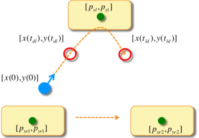
The calculation starts at the transition from the end of the single-support stage of the right foot to the double-support stage (Fig. 5). Accordingly, the time reference starts (t0= 0)
at the beginning of the double-support stage that will move the ZMP from the right foot to the left one. The end of the double-support stage,tdl, will lead to another stage of single-support. During this new stage of single-support, the ZMP will stay on the left foot, while the right foot will move to its target position. When this stage finishes (tld), the target position for
Fig. 5. Positions of the ZMP and the parameter ZMPDSF are employed to obtain the position of the CoM at the extremes of the single-support stage of the current step.
the left foot will be read, and the process will start again. The available information at t0 is summarized as follows:
• Position of the ZMP on the right foot before t0, named
pyr1.
• Position of the ZMP on the left foot, pyl, during the single-support stage (between tdl and tld), which will have the left foot as support .
• Duration tl of this single-support stage.
• Position of the ZMP on the right foot during the next single support stage, pyr2.
• Position and speed of the CoM int0, named respectively
y(0) andy˙(0).
In equation (15), the datatdl,tld,y(tdl)andy(tld)will be employed to obtain the boundary conditions that will make it possible to find the values of the constantsc1y andc2y. Since
tl is already known, it is possible to findtld=tdl+tl. As for equation (17),t0,tdl,y(t0),y˙(t0),y(tdl)andy˙(tdl) will be used for the boundary conditions. Consideringt0,y(t0)
andy˙(t0)are known, only the values oftdl,y(tdl)andy˙(tdl) need to be found.
To sum up, in order to solve equations (15) and (17), it is necessary to obtain the values oftdl,y(tdl),y˙(tdl)andy(tld). This calculation will be detailed in the following lines. Once obtained, it will be possible to calculate the position of the CoM at any time during the single-support or double-support stages of the step.
A. Calculating y(tdl) andy(tld)
The point y(tdl)is the geometric place of the CoM where the transition from the double-support stage to the single-support stage takes place. By employing the parameter ZM-PDSF, it will be possible to define the portion of distance between the feet that will be covered by the CoM in double support mode. In this manner, a hint fory(tdl)andy(tld)will be obtained. y(tauxdl ) = pyr1+ (pyl−pyr1)(0.5 + ZM P DSF 2 ) (18) y(tauxld ) = pyl+ (pyr2−pyl)(0.5− ZM P DSF 2 ) (19)
Fig. 6. The initial speed of the CoM in the simple-support stage is defined by the positions of the CoM at the beginning and at the end of this stage and by the duration of the simple-support stage (tl)
If there is a strong change in the lateral distance between the right foot and the left foot from one step to the next, there will be a large difference betweeny(tdl)andy(tld). This large difference will lead to speed peaks in one of the extremes that will cause strong accelerations of the CoM in the double support stage.
Since the position of the right foot during the next step is available, it is possible to modify the hint position for y(tdl) so that the position and the speed of the CoM at the end of the single support stage are adequate for the next step.
This is why the space in the single support stage has been distributed in a symmetric way, and the final position at the end of this stage is the same as the initial position of the next single support stage: y(tld) = y(tdl). To force this equality, the hint values calculated in (18) and (19) have been averaged.
y(tdl) =y(tld) =
y(taux
dl ) +y(tauxld )
2 (20)
B. Calculatingy˙(tdl)
The next value to be obtained is the speed of the CoM at the beginning of the single support stage, y˙(tdl), as can be observed in Fig. 6. The duration of the single support stage,
tl, and the recently calculated values ofy(tdl)andy(tld)will be employed to operate in (15).
y(tdl) =c1yeαtdl+c2ye−αtdl+py (21) Sincetld =tdl + tl,
y(tld) =c1yeαtdleαtl+c2ye−αtdle−αtl+py (22) Ifc7y andc8y are defined as follows:
c7y = c1yeαtdl (23)
c8y = c2ye−αtdl (24) Equations (21) and (21) can be rewritten in the following way:
y(tdl) = c7y+c8y+py (25)
Fig. 7. Position and speed of the CoM at the extremes of the double support stage are employed to generate a value for the duration of the double support stage.
It is possible, then, to find the values of c7y and c8y by making use of (20). Finally, by deriving (15), the expression for y˙(tdl)can be obtained:
˙
y(tdl) =αc7y−αc8y (27)
C. Calculatingtdl
The last value to be found is the duration of the double support stage. This situation is illustrated in Fig. 7. The speeds at the beginning and at the end of the single support stage,
˙
y(t0) and y˙(tdl) respectively, will be averaged to obtain a guiding value for the CoM speed during the double support stage. In this way, the value oftdlcan be found with equation (28). tdl= y(tdl)−y(t0) ˙ y(tdl)+ ˙y(t0) 2 (28) V. EXPERIMENTAL VALIDATION
This section evaluates the proposed locomotion approach. To begin with, the platform employed will be presented to-gether with the environment where the experiments take place. The following subsection is devoted to a brief explanation of the inverse kinematics algorithm for the platform Nao. Later, several experiments will be analyzed: a first group consisting of pure unidirectional movements, and a second where omnidirectional capabilities are demonstrated.
A. Experimental setup
The platform employed to validate the proposed omni-directional motion planning approach experimentally is the commercial humanoid robot Nao, developed by the French company Aldebaran Robotics. This is the platform used in the Standard Platform League of the international Robocup
Competition event.
The real world experiments are performed on a similar carpet to the official soccer field ofStandard PlatformLeague,
Fig. 8. Nao platform from Aldebaran Robotics Company.
2010 Edition, which is detailed in the official rules of such a league. The simulated experiments are performed in the Webots simulator, from Cyberbotics company. This simulator is convenient, since Aldebaran Robotics, the robot’s manu-facturer, provides a precise model of Nao platform for it. Moreover, this simulator provides dynamics simulation by making use of the Open Dynamic Engine (ODE), which permits the effect of gravitational and reaction forces to be evaluated.
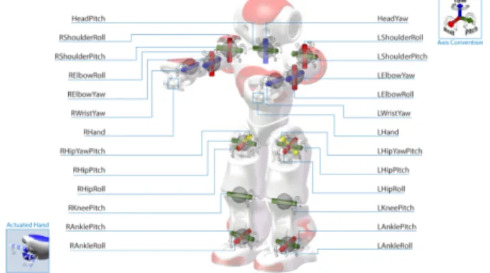
The humanoid robot Nao has 21 degrees of freedom (DoF) depicted in Fig. 8: twoDoF for the head, fourDoF for each arm and sixDoF for each leg. The number ofDoF is twenty-one because both legs share twenty-one joint, namedHipY awP itch
joint, which supposes a constraint in order to solve the inverse kinematics problem. The head joints are controlled by an active vision system depending on perceptual needs. The proposed method does not make use of any sensor, gyroscope and accelerometers available in the platform as feedback to improve the stability of the dynamic gait, i.e. the proposed method is an open-loop approach.
B. Inverse Kinematics
The inverse kinematics problem must be solved in order to calculate the joint positions for a CoM trajectory. This section describes the implementation details for this humanoid plat-form. This is the information used to calculate the sequence of joints:
• Reference system (located at the supporting leg).
• Position of the CoM (x,y,z).
• Orientation of the torso (Yaw,Pitch,Roll).
• Position of the swinging foot (x,y,z).
• Plane orientation of the swinging foot (Pitch,Roll). The inverse kinematics problem can be divided into two stages:
• Finding the pelvis position that places the CoM at its target position.
• Finding the joint values for both legs constrained to pelvis
position, torso orientation and swinging sole orientation. The approach employed to find the support side position of the pelvis assumes that the only DoFare the joints of the supporting leg. Besides, the modifications of the CoM position are negligible. The aim is to find the position of the supporting
Fig. 9. The iterative method to find the joints values given the CoM target position.
side of the pelvis that places the CoM at the desired position. The solution is obtained by using an iterative method, shown in Fig. 9, in order to decrease the position error of the inverse kinematics problem.
The analytical solution of the proposed method is described next. The method assumes that the position of the supporting side of the pelvis is known, taking the one previously obtained. For the sake of simplification, we will describe the procedure for the right leg of the robot. The reference system is placed on the right sole. The rotation axes of the joints of both legs are numerated from one (right foot) to eleven (left foot). The chain of matrices to be multiplied in order to obtain the orientation of the torso is as follows,
ROT = Rx(−α1)Ry(−α2)Ry(−α3)Ry(−α4)
Rx(−α5)Ry(−α6)Rx(−π4) (29)
where αrepresents the joints of the legs. Besides, the orien-tation of the left foot can be obtained as follows,
ROL = ROTRx(−π4)Ry(α6)Rx(α7)Ry(α8)
Ry(α9)Ry(α10)Rx(α11)
(30)
According to the sign criteria adopted, the turning sense is considered positive when the moving part of the body is farther from the torso. Since the reference system moves from one foot to the other, the sign criterion for the turning sense of the joints must be changed. Therefore, the sign of the joints is negative when the reference system is in the right leg. Theα
values corresponding to the HipRolljoints have been merged with an extra rotation in order to simplify the calculation. This simplification consists of orientating the y axis of this joint parallel to the HipYawPitchjoint as follows,
Fig. 10. Forward walking experiment. In the upper row, the height of the left foot (+) and right foot (o) is shown. The second and third rows show the evolution of the CoM (continuous curve) and the ZMP (*) in the frontal and sagittal planes respectively.
RAnkleRoll α1 RAnklePitch α2 RKneePitch α3 RHipPitch α4 RHipRoll α5+π4 RHipYawPitch α6 LHipYawPitch α6 LHipRoll α7−π4 LHipPitch α8 LKneePitch α9 LAnklePitch α10 LAnkleRoll α11
The first angles to be obtained are those of the right leg of the robot (ankle and knee). These three angles enable the robot to place the support side of the hip at its target position. Once we have obtained the joint valuesα1,α2 andα3, we can use
(29) to calculate the joint anglesα4,α5andα6 by identifying
the terms in the resulting matrix from the left members of (33), RRT high=Rx(−α1)Ry(−α2)Ry(−α3) (31) ROT =RRT highRy(−α4)Rx(−α5)Ry(−α6)Rx(− π 4) (32) RtRT highROTRx(− π 4) t=R y(−α4)Rx(−α5)Ry(−α6) (33)
Fig. 11. Horizontal plane of CoM trajectory in a forward walking trajectory.
where we have made use of the property of rotation matrices in which inverse matrix is similar to its transpose.
Once the position and orientation of the swinging side of the hip and the position of the swinging ankle are known, it is possible to make use of the initial target information to find the joint values of α7, α8 and α9. Finally, the α10 and α11
joint angles are obtained by updating the orientation of the reference frame and comparing it to the required orientation of the sole plane of the left foot.
C. Walking pattern experiments
This section shows the trajectories of two different walking patterns that make use of the proposed motion planning algorithm. These walking patterns are pure forward and lateral straight movements of the robot, since they allow us to illustrate clearly the behavior of the ZMP.
The height of the CoM will be fixed at 235mm, and a sam-pling time of 40ms is employed to generate the trajectories. In this case, the experiments are only tested on the Webots simulator.
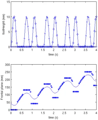
In the first experiment, the robot walks straight in the forward direction, while the behavior of the CoM and the ZMP is analyzed. This is illustrated in Fig. 10. The first row indicates the height of the feet. When the circle points have a value above zero, it means that the right foot is in the air, therefore the left foot is the support-foot. In this case, the ZMP should stay still on the left foot. The opposite happens when the cross points are the ones which have a positive value. On the other hand, if no foot is in the air, the ZMP is constrained to stay at any place between both of the feet, that is, within the convex hull.
In the second row of Fig. 10, the lateral component of the evolution of the CoM is shown. The ZMP position is marked with star points. Since the lateral coordinates of the feet are constant (0 for the left foot and 100 for the right one), we note that the ZMP stays on the support foot during the single-support stages and that it moves between the feet during double-support stages.
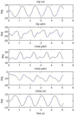
Fig. 12. Position of joints of left leg during forward walking experiment.
The bottom row of Fig. 10 shows this time the evolution of the CoM and the ZMP in the sagittal plane. Once again, the ZMP stays still during the single support stage and moves along the convex hull during the double-support stage. The slope of the curve plotted here is the forward speed of the robot.
Fig. 11 is a combination of the sagittal and frontal move-ment of the CoM plotted in Fig. 10. This time, the trajectory of the CoM in the horizontal plane is given. In order to get a timing reference, the distance between samples must be observed, since both axes refer to spatial information. The fact that the samples which are around the lateral extremes of the trajectory are closer than the ones in the middle, indicates that the CoM movement is slower during single support stages and faster during double support ones.
Fig. 12 and Fig. 13 show the joint position and the joint speed respectively when the robot is following a forward trajectory. We can observe in Fig. 13 that the joint speed is bounded at 100 degrees/sec, which can help to visualize the pace of the movements. Additionally, it is important to note that we do not appreciate any discontinuity in the joint speeds. This is one of the goals of the design of the locomotion system in order to provide smooth movements to the gait which increase stability.
Fig. 13. Speed of joints of left leg during forward walking experiment.
lateral one. Analogously to Fig. 10, the evolution of CoM and ZMP trajectories are displayed (below) together with the height of the feet (above). In this case, a graph for the sagittal plane component of the movement is not shown, since its value is constant. We can also observe that the ZMP is kept between both feet during the double support stage, so ensuring stability. The average slope of the curve displayed in the lower graph is the average lateral speed of the robot.
D. Omnidirectional experiment
The above experiments have demonstrated the stability of the robot while performing pure forward and lateral move-ments. The next step in order to get an omnidirectional loco-motion is to incorporate turning capabilities and simultaneous combination of the previous walking patterns. That will be the target of the next experiment: the circular walking.
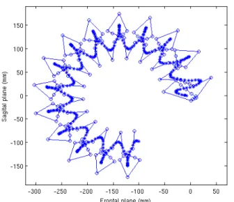
Fig. 15 shows the trajectory of the CoM and the ZMP in the horizontal plane while the robot walks describing a circle. The CoM trajectory is the smooth curve described by the star points. The ZMP trajectory (circle points) can be divided in three groups of samples: an inner ring, an outer ring and a regular pattern of samples enclosed within this two rings. The inner and outer rings are formed by the ZMP positions on the left and the right foot respectively during the single-support
Fig. 14. Lateral walking experiment. In the upper graph, the height of the left foot (+) and right foot (o) is shown. The lower graph shows the evolution of the CoM (continuous curve) and the ZMP (*) in the frontal and plane.
stages. The samples enclosed within these rings belong to the double-support stages of the walking. It is important to notice that the double support samples are far from the region delimited by the single-support samples, so avoiding instability risks.
The temporal evolution of the trajectories is difficult to extract from the figure, since it is not explicitly shown. For instance, during the single-support stages, the ZMP samples overlap, resulting in a single point in the plot for all the samples of every single-support stage.
The final feature to be evaluated in the proposed method is the capability of linking different trajectories dynamically, which will be tested in the last experiment. In this test, the real robot is follows an online generated walking pattern during 10 seconds. At that time, the gait is forced to follow a new walking pattern abruptly. The different stages of the experiments are: forward walking, smooth curve to the left (5 degrees per step), stronger curve to the right (20 degrees per step), forward walking again and left sense turning (30 degrees per step). Fig. 16 shows the trajectories followed by the robot in the transverse plane. We can observe the transitions between walking patterns, and how the proposed approach solves the problem by generating smooth and continuous trajectories.
VI. CONCLUSION ANDFUTUREWORK
This paper has presented the motion planning approach used to generate online dynamical stable trajectories of the CoM of a humanoid robot that adapts to the omnidirectional walking
Fig. 15. Circular walking experiment. Trajectory of the CoM (star points) and the ZMP (circle points) in the transverse plane.
Fig. 16. Omnidirectional walking experiment. Different walking patterns are linked ensuring analytically stability.
patterns followed by its feet. The method has been designed to provide humanoids with the capability of fast reaction when environment changes rapidly, which is of special interest in dynamic and/or uncertain environments. The implementation of the method is focused on efficiency to meet the hard real-time constraints in this kind of applications. Currently, the omnidirectional gait is not optimized for velocity, but it can be used for specific tasks, such as approaching an object or po-sitioning humanoids for accurate operations. The experimental
walking direction and orientation without stopping.
Future efforts will be focused on closing the loop control by making use of the gyroscope and the accelerometers sensors that incorporate the platform. Besides, stability can be improved using rhythmic patterns for arms, depending on the CoM trajectories.
ACKNOWLEDGEMENT
This work has been supported by Spanish Ministry of Sci-ence and Innovation under DPI-2007-66556-C03-02 CICYT project and by Spanish Ministry of Education through its FPU program.
REFERENCES
[1] T. Kalm´ar-Nagya, R. D’Andrea, and P. Ganguly,Near-Optimal Dynamic Trajectory Generation and Control of an Omnidirectional Vehicle, Robotics and Autonomous Systems, 46(1):47–64, 2004.
[2] B. Hengst, S.B. Pham, D. Ibottson, and C. Sammut,Omnidirectional Locomotion for Quadruped Robots, RoboCup 2001: Robot Soccer World Cup V, Lecture Notes in Computer Science, vol. 2377, pp. 73–94, 2002. [3] K. Kamikawa, T. Arai, K. Inoue, and Y. Mae,Omni-directional Gait of Multi-Legged Rescue Robot, in Proc. of IEEE Int. Conf. on Robotics and Automation (ICRA), pp. 2171–2176, New Orleans, LA, USA, 2004. [4] S. Behnke, Online Trajectory Generation for Omnidirectional Biped
Walking, in Proc. of IEEE Int. Conf. on Robotics and Automation (ICRA), pp. 1597–1603, Orlando, Florida, USA 2006.
[5] Qiang Huang, K. Yokoi, S. Kajita, K. Kaneko, H. Arai, N. Koyachi, and K. Tanie,Planning Walking Patterns for a Biped Robot, in IEEE Transactions on Robotics and Automation, 17(3):280–289, 2001. [6] M. Vukobratovi´c, A.A. Frank, and D. Juricic, On the Stability of
Biped Locomotion, in IEEE Transactions on Biomedical Engineering, 17(1):25–36, 1970.
[7] S. Kajita, F. Kanehiro, K. Kaneko, K. Yokoi, and H. Hirukawa,The 3D Linear Inverted Pendulum Model: A Simple Modeling for a Biped Walk-ing Pattern Generation, in Proc. of IEEE/RSJ Int. Conf. on Intelligent Robots and Systems (IROS), pp. 239–246, Maui, Hawaii, USA, 2001. [8] Y. Breniere, and C. Ribreau,A Double-Inverted Pendulum Approach of
the Human Gait, Journal of Biomechanics, 31(1):86–86, 1998. [9] A.J. Ijspeert, “Central Pattern Generators for Locomotion Control in
Animals and Robots: A Review”, Neural Networks, 21(4):642–653, 2008.
[10] G. Endo, J. Morimoto, T. Matsubara, J. Nakanishi, and G. Cheng,
Learning cpg-based biped locomotion with a policy gradient method: Application to a humanoid robot, Int. Journal of Robotics Research, 27(2):213228, 2008.
[11] S. Kajitak, F. Kanehiro, K. Kaneko, K. Fujiwara, K. Harada, K. Yokoi and H. Hirukawa,Biped Walking Pattern Generation by using Preview Control of Zero-Moment Point, in Proc. of IEEE Int. Conf. on Robotics and Automation, Taipei, Taiwan, 2003.
[12] S. Czarnetzki, S. Kerner, O. Urbann, Observer-based dynamic walk-ing control for biped robots, in Robotics and Autonomous Systems 57(8):839–845, 2009.
[13] K. Harada, S. Kajitak, K. Kaneko and H. Hirukawa, An analytical Method on Real-time Gait Planning for a Humanoid Robot, in Proc. of IEEE/RAS Int. Conf. on Humanoids Robots 2, pp. 640–655, Los Angeles, CA, USA, 2004.
[14] S. Kajitak, F. Knaehiro, K. Kaneko, K.Yokoi and H. Hirukawa,The 3D Linear Inverted Pendulum Mode: A simple modeling for a biped walking pattern generation, in Proc. of 2001 IEEE/RSJ Int. Conf. on Intelligent Robots and Systems, pp. 239–246, Maui, Hawai, USA, 2001.